A component based approach to power system applications development
7
0
0
Texte intégral
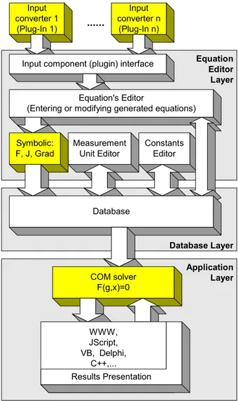
(2) 14th PSCC, Sevilla, 24-28 June 2002. Session 33, Paper 1, Page 2. includes information about the mathematical model of the system, its symbolic Jacobian, and initial guesses. Thus, time needed for parsing and symbolical differentiation is removed from the application layer. Information on the current system state is entered using editor and input format converters. The application layer can use this data via component models. 2.1 Code reusability Once designed, implemented and tested application (component) should be re-used whenever possible. Implementation of applications with code reusability intentions requires that the design process be dominant in the software development cycle. It is natural for an objectorientated approach to go from the general (even abstract) toward the specific. The paper uses this approach to achieve code reusability. A general-purpose solver that solves non-linear sets of equations is implemented as the main part of this approach. Since a general-purpose solver cannot know in advance what kind of problem is going to be solved, the solver must be able to perform symbolic evaluations. The symbolic module is responsible for evaluating functions, gradients, Jacobians, and Hessians of the specific problem. The solver component is based on a well-tested and documented SolverQ implementation [5,6]. Since this solver makes extensive use of symbolic computation, its native format is used as input to the solver. For power systems, on the other hand, there are specific data input formats (e.g. CDF, PTI) that are frequently used. In order to reuse these power system file formats, converters for each format type are implemented. These converters generate the same input format for the solver. Developers can use these modules as part of the solution process, or can use them as independent stand-alone modules. Furthermore, these converters help in seamlessly integrating component models and the proposed framework into existing power system model organizations. Since components are used and distributed in binary formats there is no need for recompilation of application. Future applications can be developed with additional flexible features. Specific input format. Input Format Adaptation. 2.2 Application robustness and input data reusability Introducing symbolic evaluation and having application based on a general solver results in reduced computational speed. In order to speed up the solving process, a prepared Jacobian and parsed input data are used. This is implemented using formula (module) pool, which contains unique formula (system) names and information needed by the solver. Thus, unnecessary parsing for repetitive solving of the same problem is skipped. For on-line adjustment, parameter variables are included. Figure 2. contains the design of the proposed framework. New components are emphasized in yellow. Input converter 1 (Plug-In 1). ....... Input converter n (Plug-In n) Equation Editor Layer. Input component (plugin) interface. Equation's Editor (Entering or modifying generated equations). Symbolic: F, J, Grad. Measurement Unit Editor. Constants Editor. Database. Database Layer COM solver F(g,x)=0. Parameter data and initial guesses Plug-in. General purpose solver. To be robust, future applications have to implement a plug-in loader module. This module collects all available plug-ins for different problems. Using this approach, a main application does not need to be recompiled or even changed to accommodate additional requirements. From a developer’s point of view there is only a need for a new plug-in (converter) implementation. A plug-in contains descriptions that are required by the user interface. Thus, plug-ins must “expose” all information necessary for dynamic menu construction and information on required file format extensions.. Results. Figure 1: Input data adaptation for general purpose solver. WWW, JScript, VB, Delphi, C++,... Results Presentation. Figure 2: Framework for using COM modules. Application Layer.
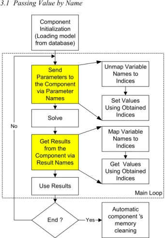
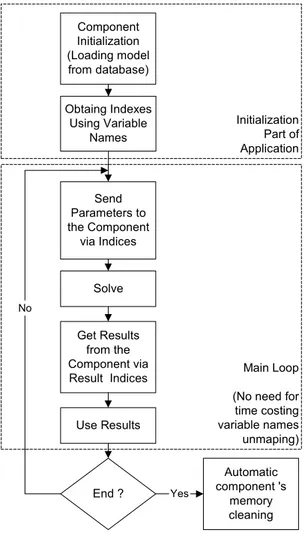
(3) 14th PSCC, Sevilla, 24-28 June 2002. Session 33, Paper 1, Page 3. In order to obtain input data model reusability three layers are introduced. An Equation Editor Layer contains all plug-ins and an editor for manually entering and changing models. This layer also includes an editor for constants and an editor for unit conversion. The database layer is used for storing models for future use. The database is organized as a tree. The application layer contains specific user's code and results presentation obtained from the COM solver. The Equation Editor prepares set of equations, parses them, and stores them in an appropriate format into the database. This process can require either manual typing or using available plug-ins for converting data from other input formats. The Equation Editor produces postfix notation for faster formula evaluation. The Measurement Unit Editor stores information needed for unit conversion. This information is used by the application layer for unit conversions. The Constants editor enters values for the most useful constants and stores information into the database. The Appendix contains screenshots of these parts of framework. Once every has been organized, the COM solver requires very short overhead time. The COM solver exposes its interface to the Application Layer for setting parameter variables (g) and for taking solutions (x). 2.3 Generic approach for future development Three different components are developed: converters, component for parsing and symbolic derivation, and a non-linear solver. These three components are taken directly from SolverQ code. The flexibility of this framework is illustrated on the following Figure, where components are used without a database layer. Specific converter. Symbolic: F, J, Grad. Solver F(g,x)=0. Figure 3: Component piping. Figure 3 shows in a simple and generic way how to obtain a solution on a specific problem in power system. However, greater robustness of application can be obtained if database layer is included, as described next. 3. COM SOLVER USAGE. The COM Solver is developed using C++ and ATL. This leads to small memory requirements for executable components. Components can be used and controlled by external clients (e.g. VBScript, JScript, VBA, VB, VC++, etc.), even on web pages. There are three different ways of using the COM solver. These differences are caused by the way in which parameters and variable values are passed. Parameter and variable values passing can be done using names or indices. The Appendix contains a partial listing of the solver component interface.. 3.1 Passing Value by Name Component Initialization (Loading model from database). Unmap Variable Names to Indices. Send Parameters to the Component via Parameter Names. Set Values Using Obtained Indices. Solve No. Map Variable Names to Indices. Get Results from the Component via Result Names. Get Values Using Obtained Indices. Use Results Main Loop. End ?. Yes. Automatic component 's memory cleaning. Figure 4: Passing values by variable names. The highlighted part of the example shows lines of code that pass parameter values by names. Named parameter passing is very flexible from a developers' point of view. The code is more flexible in case the model is modified. However, this method incurs some overhead time needed for mapping names to actual memory locations. Using this method of passing values into solver component should be avoided inside of loops. 3.2 Passing Value by Index This is the fastest approach for passing parameters inside and outside of COM modules. From a developers' point of view this method is less clear. There is a need for using comments for each index. Problems can arise when models are changed or when the order of variables is reorganized. In order to use fast data access of passing values by index and flexibility of passing values by names, a combination of these two methods is used. 3.3 Combination of Passing Values by Name and Index Combination of passing values by name and by index solves the problem of potential variables reordering with the same time response. To obtain this, developer should use GetParamIndex and GetOutputIndex in initializating part of application code. Thus, an application will obtain indices at run time and can use them in loops..
(4) 14th PSCC, Sevilla, 24-28 June 2002. Session 33, Paper 1, Page 4. 0.6* k=v3* (+v6* (-1.923077)* COS(a3-a6)+v6* 9.615385* SIN(a3-a6) +v5* (-1.463415)* COS(a3-a5)+v5* 3.170732* SIN(a3-a5)+ v3* 4.155722+v2* (-0.769231)* COS(a3-a2)+v2* 3.846154* SIN(a3-a2));. Component Initialization (Loading model from database) Obtaing Indexes Using Variable Names. Initialization Part of Application. (-0.7)* k=-v5* (+v6* 3* COS(a5-a6)-v6* (-1)* SIN(a5-a6)+v4* 2* COS(a5-a4)-v4* (-1)* SIN(a5-a4)+v3* 3.170732* COS(a5-a3)-v3* (-1.463415)* SIN(a5-a3)+v2* 3.000000* COS(a5-a2)-v2* (-1)* SIN(a5-a2)+v5* (-14.210265)-v5* 5.293290* SIN(a5-a5)+v1* 3.112033* COS(a5-a1)-v1* (-0.829876)* SIN(a5-a1));. Solve No. Get Results from the Component via Result Indices. Main Loop (No need for time costing variable names unmaping). Use Results. Yes. Automatic component 's memory cleaning. Figure 5: Combined way of passing values. 4. RESULTS. Components are tested on power flow and economic dispatch problem. Timing results are given for power flow compared to MatPower [14]. 4.1 Power Flow problem As a demonstration of the modeling process, a 6-bus system is chosen. Listing 1 shows output from the converter, which uses common data format file (CDF) and transforms data into form that can be solved using COM solver. These data are used as an input for the symbolic COM solver. {Generated from CF File} {Problem: Power Flow} k=1.0; a1=0.0; v1=1.05; 0.5* k=v2* (+v6* (-1.559020)* COS(a2-a6)+v6* 4.454343* SIN(a2-a6) + v5* (-1)* COS(a2-a5)+v5* 3* SIN(a2-a5)+ v4* (-4)* COS(a2-a4) +v4* 8* SIN(a2-a4)+v3* (-0.769231)* COS(a2-a3) + v3* 3.846154* SIN(a2-a3)+ v2* 9.328251+ v1* (-2)* COS(a2-a1)+ v1* 4* SIN(a2-a1)); v2=1.05;. (-0.7)* k=-v4* (+v5* 2* COS(a4-a5)-v5* (-1)* SIN(a4-a5)+v2* 8* COS(a4-a2)-v2* (-4)* SIN(a4-a2)+v4* (-14.670882)-v4* 6.176471 * SIN(a4-a4)+v1* 4.705882* COS(a4-a1)-v1* (-1.176471)* SIN(a4-a1)); (-0.7)* k=v5* (+v6* (-1)* COS(a5-a6)+v6* 3* SIN(a5-a6)+v4* (-1)* COS(a5-a4)+v4* 2* SIN(a5-a4)+v3* (-1.463415)* COS(a5-a3)+v3* 3.170732* SIN(a5-a3)+v2* (-1)* COS(a5-a2)+v2* 3* SIN(a5-a2)+v5* 5.293290+v1* (-0.829876)* COS(a5-a1)+v1* 3.112033* SIN(a5-a1));. Send Parameters to the Component via Indices. End ?. v3=1.07; (-0.7)* k=v4* (+v5* (-1)* COS(a4-a5)+v5* 2* SIN(a4-a5) +v2* (-4)* COS(a4-a2)+v2* 8* SIN(a4-a2)+v4* 6.176471+v1* (-1.176471)* COS(a4-a1)+v1* 4.705882* SIN(a4-a1));. (-0.7)* k=v6* (+v5* (-1)* COS(a6-a5)+v5* 3* SIN(a6-a5)+v3* (-1.923077) * COS(a6-a3)+v3* 9.615385* SIN(a6-a3)+v6* 4.482097+ v2* (-1.559020)* COS(a6-a2)+v2* 4.454343* SIN(a6-a2)); (-0.7)* k=-v6* (+v5* 3* COS(a6-a5)-v5* (-1)* SIN(a6-a5)+v3* 9.615385 * COS(a6-a3)-v3* (-1.923077)* SIN(a6-a3)+v6* (-17.037228)-v6* 4.482097* SIN(a6-a6)+v2* 4.454343* COS(a6-a2)v2* (-1.559020)* SIN(a6-a2)); {Initial values:} v1≈1.000000; a1≈0.000000; v3≈1.000000; a3≈0.000000; v5≈1.000000; a5≈0.000000;. v2≈1.000000; v4≈1.000000; v6≈1.000000;. a2≈0.000000; a4≈0.000000; a6≈0.000000;. Listing 1. Output from CF converter module (6-bus). Last output lines contain symbol “≈”, which denotes initial values. Symbol “;” is used as separator between equations. Symbols “{“ and “}“ denote start and end of a comment section, respectively. Prepared data are sent to the symbolical differentiator, which constructs symbolical Jacobian. Both, symbolical Jacobian and function equations are transformed into postfix evaluators, which will be used by NewtonRaphson solver. Listing 2. contains solution obtained after solving 6 bus problem. Solution is obtained in 2 iterations and tolerance = 1e-3. v1=1.050000 v3=1.070000 v5=0.979665. a1=0.000000 a3=-0.075642 a5=-0.091175. v2=1.050000 v4=0.986423 v6=1.014433. a2=-0.065010 a4=-0.072934 a6=-0.104205. Listing 2. Solution of 6-bus power system. In presented example, components are “piped” forming the following chain: problem formulation (CDF file) → power flow converter → symbolical differentiator → Newton-Raphson solver. Data transferred through components, are available for examination. Listing 1. contains data transferred from converter component into symbolical differentiator. In case when data are accessed from database, complete solver construction process is much faster since database contains prepared postfix evaluators, which are loaded directly into the solver..
(5) 14th PSCC, Sevilla, 24-28 June 2002. Authors cannot show data passed from symbolical evaluator into the solver, due to paper’s space restriction. However, an example of output from a symbolical differentiator is shown on the following example. 4.2 Economic Dispatch problem For clarity reasons, Wood-Wollenberg’s economic dispatch example will be examined. In order to solve this problem, augmented Lagrangian converter will be put in front of symbolical differentiator and solver components chain. Economic dispatch problem solution is obtained via four “piped” components. Original problem formulation is passed through the following component chain: problem formulation → Lagrangian converter → symbolical differentiator → (Hessian) symbolical differentiator → Newton-Raphson solver. Problem formulation is shown on the following listing. {Minimize:} 1.1* (510+7.2* p1+0.00142* p1^2)+0.00194* p2^2+7.85* p2+0.00482* p3^2+7.97* p3+388; {Subject to:} p1 + p2 + p3 = 850 + ploss; {and} ploss = 0.00003 * p1^2 + 0.00009 * p2^2 + 0.00012 * p3^2; {Inequality constraints:} p1 < 400; p2 < 300; p3 < 300. Listing 3. Economic dispatch problem formulation. Lagrangian converter converts inequality constraints into equality constrains and constructs augmented Lagrangian. Listing 4. contains output from Lagrangian converter for economic dispatch problem. {Augmented Lagrangian:} {L=}µ6* (SQUARE(δ6)+p3-300)+µ5* (SQUARE(δ5)+p2300)+µ4* (SQUARE(δ4)+p1-400)+µ3* (ploss-(0.00003* p1^2+ 0.00009* p2^2+0.00012* p3^2))+µ2* (p1+p2+p3-(850+ploss))+ 1.1* (510+7.2* p1+0.00142* p1^2)+0.00194* p2^2+7.85* p2+0.00482* p3^2+7.97* p3+388;. Listing 4. Output from Lagrangian converter. Output from Lagrangian converter is sent to the symbolical differentiator, which finds derivatives with respect to each variable. {d(L)/d(p3)=} µ6+µ3* (-0.00012* p3* 2)+µ2+0.00482* p3* 2+7.97; {d(L)/d(p2)=} µ5+µ3* (-0.00009* p2* 2)+µ2+0.00194* p2* 2+7.85; {d(L)/d(p1)=} µ4+µ3* (-0.00003* p1* 2) + µ2+ 1.1* (7.2+0.00142* p1* 2); {d(L)/d(ploss)=} µ3+(-µ2); {d(L)/d(µ2)=} p1+p2+p3-(850+ploss); {d(L)/d(µ3)=} ploss-(0.00003* p1^2+0.00009* p2^2+0.00012* p3^2); {d(L)/d(δ4)=} µ4* δ4* 2; {d(L)/d(µ4)=} SQUARE(δ4)+p1-400; {d(L)/d(δ5)=} µ5* δ5* 2; {d(L)/d(µ5)=} SQUARE(δ5)+p2-300; {d(L)/d(δ6)=} µ6* δ6* 2; {d(L)/d(µ6)=} SQUARE(δ6)+p3-300;. Listing 5. Output from symbolical differentiator. From this point on, situation is the same as previously described power flow problem. Symbolical data, shown. Session 33, Paper 1, Page 5. on Listing 5, are sent to the Hessian differentiator. Hessian differentiator evaluates symbolical Hessian of given problem. During solving, Hessian will play role of Jacobian in Newton-Raphson solver. The following listing contains solution of stated problem. Solution is obtained in 5 iterations, and tolerance = 1e-3. p1=334.2882655 ploss=19.1153997 µ4=-1.19*10-9 δ4=8.1062776. p2=234.8271323 µ2=-9.1477966 µ5=0.0000002 δ5=8.0729727. p3=300.0000000 µ3=-9.1477966 µ6=-2.3728448 δ6=6.44*10-9. Listing 6. Economic dispatch solution. 4.3 Timing results Table 1 shows results of the COM power flow solver module computation as compared to MatPower [14] execution times. Input model IEEE118 IEEE300. Tolerance 10-6 10-6. COM solver No. Iter. Time 3 0.210 4 1.580. MatPower No.Iter. Time 3 0.05 5 0.16. Table 1. Testing platform: Win2000, Pentium III, 750 MHz. The execution time is bigger for COM due to the use of a general nonlinear solver for the set of equations. Furthermore, symbolic evaluation requires extensive stack usage and parsing time. However, despite the fact that symbolical evaluation is used inside of components, computational speed is still quite tolerable, about 10 times slower than the “hard coded” approach. In other larger examples this same ratio seems to hold 5. CONCLUSIONS AND FUTURE WORK. A new approach for component based application development in power system has been explored. A generic framework for power system models organization and software development has been proposed. Using code reusability as one of its main guidelines, components for future software development has been developed and tested. Fast technological development was taken into consideration, so that computational speed of future applications was not the main goal. Instead of speed of execution, speed of development is the paramount. Examples shown in this paper emphasize simplicity and efficiency of development. Developers are not bounded by a programming language. Proposed COM modules enable future software development using different programming languages. Even developers with limited power system knowledge can use these components very efficiently. Since COM modules are created using C/C++ and ATL (and thus, they are very "light" in terms of memory consumption) they can be used on web pages, and embedded within script languages that support COM..
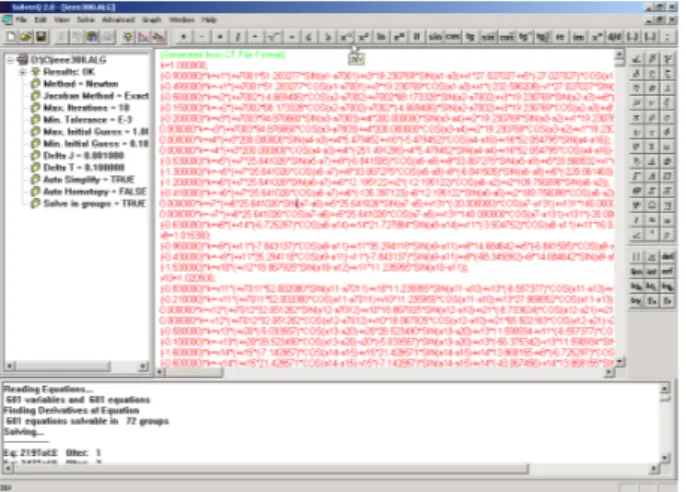
(6) 14th PSCC, Sevilla, 24-28 June 2002. The problem of model redesign and the need for complete application recompilation has been removed using a centralized database for model collection. Applications developed within this framework only need to be restarted to re-initialize needed COM modules. Collecting updates on model changes is much easier using this framework. There is a sacrifice in speed for this flexibility. A slowdown of a factor of 10 is seen in those applications illustrated as well as a few others. Computing power, however, is making such considerations less relevant. Future work will try to add more robust optimization composers, such as Interior-Point solver. REFERENCES [1] A. F. Neyer, F. F. Wu, K. Imhof, "Object-oriented Programming for Flexible Software: Example of Load Flow", IEEE Transactions on Power Systems, Vol. 5, No 3. August 1990, pp. 689-696 [2] Mike Foley, Anjan Bose, "Object-oriented On-line Network Analysis", IEEE Transactions on Power Systems, Vol. 10, No. 1, February 1995, pp. 125-132 [3] E. Z. Zhou, "Object-oriented Programming, C++ and Power System Simulation", IEEE Trans. on Power Systems, Vol. 11, No. 1, February 1996. pp. 206-215 [4] E. Handschin, M. Heine, D. König, T. Nikodem, T. Seibt, R. Palma, "Object-oriented Software Engineering for Transmission Planning in Open Access Schemes", IEEE Transactions on Power Systems, Vol. 13, No. 1, February 1998, pp. 94-100 [5] F. Alvarado, "Solver-Q, Equation Handler, Version 1.90", User's Manual, University of Wisconsin, ECE Department, November 1993. Session 33, Paper 1, Page 6. [6] F. Alvarado, I. Džafić, M. Glavić, "SolverQ, Equation Handling Software, Version 2.5 for Windows Operating Systems", September 2001, (limited version 2.0 is available from: http://www.untz.ba/idzafic/solverq.htm [7] Rainer Bacher, "Symbolically Assisted Numeric Computations for Power System Software Development", 13th PSCC Proceedings, pp. 5-16, June 1999 [8] Christian Bischof, Alan Carle, Peyvand Khademi, Andrew Murer, "The ADIFOR 2.0 System for the Automatic Differentiation of Fortran 77 Programs", CRPC Technical Report CRPC-TR94491, 1994 [9] Christian Bischof, Lucas Roh, Andrew Mauer-Oats, "ADIC: An Extensible Automatic Differentiation Tool for ANSI-C", Argonne National Laboratory, ANL/MCS-P626-1196, May 1997. [10]Kundur P.: Power System Stability and Control, Mc Graw-Hill Inc., 1994. [11]F. L. Alvarado, D. J. Ray: Symbolically Assisted Numeric Computation in Education, International Journal of Applied Engineering Education, Vol. 4, No. 6, 1988, pp. 519-536. [12]F. L. Alvarado, Y. Liu: General Purpose Symbolic Simulation Tools for Electric Networks, IEEE Trans. on Power Systems, Vol. 3, No. 2, 1988, pp. 689-697. [13]F. L. Alvarado, R. H. Lasseter, Y.Liu: An Integrated Engineering Simulation Environment, IEEE Trans. on Power Systems, Vol.3, No. 1, 1988, pp. 245-253. [14]Ray D. Zimmerman, David Gan: “MATPOWER, MATLAB™ Power System Simulation Package”, Version 2.0, http://www.pserc.cornell.edu/matpower/. APPENDIX Appendix contains component solver interface, screenshot of Equation Editor Module – SolverQ, and screenshots of additional tools previously mentioned in the paper. 5.1 COM Solver Module Interface COM Newton-Raphson solver module is done using dual interface automation server. All COM-aware programming languages like VB, VBA, VC++, etc. can use the automation server. HRESULT InitByStr([in] BSTR strEquationName) HRESULT InitByID([in] long nID) HRESULT GetOutputName([in] long nIndex,[out, retval]BSTR *strVarName). HRESULT GetOutputIndex([in] BSTR strVarName,[out, retval]long *nIndex) HRESULT GetAllOutputNames([out, retval] SafeArray(BSTR) *strVarNames) HRESULT GetOutputValueByName([in]BSTR strVarName, [out, retval] double *dblVarValue) HRESULT GetOutputValueByIndex([in]long nIndex, [out, retval] double *dblVarValue) HRESULT GetAllOutputValues([out, retval] SafeArray(double) *dblVarValues) HRESULT GetParamName([in] long nIndex, [out, retval] BSTR *strParamName) HRESULT GetParamIndex([in] BSTR strParamName, [out, retval] long *nIndex) HRESULT GetAllParamNames([out, retval] SafeArray(BSTR) *strParamNames).
(7) 14th PSCC, Sevilla, 24-28 June 2002. HRESULT SetParamValueByName([in] BSTR strParamName, [in] double dblParamValue). Session 33, Paper 1, Page 7. together with their belonging conversions are stored in database.. HRESULT SetParamValueByIndex([in] long nIndex, [in] double dblParamValue) HRESULT SetAllParamValues([in] SafeArray(double) *dblParamValues) HRESULT SetOutputUnit([in] long nIndex,[in] BSTR strUnitName) HRESULT Solve() Listing 7. A part of COM solver interface (MS IDL) Figure 7: Measurement Unit Module. 5.2 Equation Editor Module Using Equation Editor module, models can be edited and stored into database. This module is small modification of SolverQ. The module implements container for plug-ins and enable model designer to test the model. After testing, model can be saved into database. Saved model contains symbolical information needed in solving process.. This information can be used with method SetOutputUnit. COM based solver will automatically convert measurement unit into desired one. 5.4 Model Browser Module The following picture contains screenshot of Model Browser module.. Figure 8: Model Browser module Figure 6: Equation Editor Module. 5.3 Measurement Unit Module This module is used for data measurement unit conversion. In fact this is a very simple dialog with possibility to enter conversion equation. Information about units. This module is a helping tool for finding appropriate module inside database. The tool should help developers while making new power system applications using stored power system models..
(8)
Figure
Documents relatifs
The net result is that we have as many distinct reduced O-blades (for instance those obtained by reducing the ones associated with the triple ppsρ, sρ ` δq Ñ λ)) as we have distinct
behaviour, locomotor activity, olfactory preference and ERK phosphorylation in the mPOA of sexually 634.
L’application du modèle a été mise en oeuvre pour une culture de blé et de maïs, à partir de pratiques agricoles réelles fournies par la base de données APOCA
the curves indicate that the layer close to the wall rapidly adjusts itself to local conditions. The disturbed portion of the profile is dominated by the local wall
Pour un engin ins- table jugé facile (Niveau 1), un effet significatif de l’entrainement sur la performance de l’équilibre a été observé après six
Composite component classes differ from primitive components in that their implementation is not defined by a single class but by an embedded architecture configura- tion, i.e., a
[ 1 ], compar- ing oncological outcomes between video-assisted thoracoscopic surgery (VATS) lobectomy and open lobectomy for non-small-cell lung cancer (NSCLC) using propensity
CALICO is a model-based framework that enables the design and debug of systems in an iterative and incre- mental way, bridging a little more the gap between component-based
