10th World Congress on Structural and Multidisciplinary Optimization May 19 - 24, 2013, Orlando, Florida, USA
Shape optimization of periodic microstructures subject to stiffness and local
stress constraints
L. No¨el, L. Van Miegroet and P. Duysinx
University of Liege: Department of Aerospace and Mechanical Engineering Chemin des Chevreuils 1, B52, 4000 Liege, Belgium
Corresponding author: Lise.Noel@ulg.ac.be
1. Abstract
As suggested by Sigmund, material tailoring can be formulated as a structural optimization problem. However microstructural geometries can be rather complex while optimization process may introduce large shape modifications of boundaries and material interfaces. To circumvent the technical difficulties of classical shape optimization relying on numerous and tedious CAD model manipulations and remesh-ing, the Level Set description combined with a non-conforming XFEM analysis is a promising approach. In the present work, this approach that has been developed in work by Van Miegroet is extended to the investigation of periodic microstructures subject to compliance or stress constraints. The approach is illustrated on the famous problem of the Vigdergauz microstructure.
2. Keywords: Shape Optimization, Level Set Description, XFEM, Periodic Microstructure, Vigdergauz Microstructure
3. Introduction
Material tailoring can be formulated as a structural optimization problem as shown by Sigmund [1]. Microstructural geometries can be rather complex. Level Set description is an efficient way to deal with complex geometries [2], especially when working with realistic data coming from imaging.
Using classical finite element method (FEM) to carry out shape optimization may be arduous when dealing with complex geometries and redesign problems. Each modification of the geometry leads to frequent remeshing. Recently Van Miegroet [3] presented an interesting approach based on the Level Set description and extended finite element method (XFEM) for shape optimization. In fact, combining fixed mesh methods and non conforming finite element approximation with Level Set description exhibit several advantages. Discontinuities and interfaces can be meshed in a non conform way and a fixed mesh can be used. Therefore remeshing operations can be avoided.
In this paper, we tackle the problem of microstructural design. Material tailoring problems are expressed as shape optimizations problems subject to effective properties constraints.
4. Formulation of the optimization problem
The formulation of the studied problem is very close to the one encountered in classical finite element shape optimization. The principal advantage of the combined use of Level Set description and XFEM is that analyses can be performed on a fixed mesh. So no remeshing operations are needed. As Level Sets describe inner interfaces and boundaries of the structure, Level Set parameters are used as design variables. The goal of the optimization problem is to find the optimal shape of the structure that minimize a chosen objective function while fulfilling several design restrictions. The general formulation of this problem is given in Eq.(1).
min
x f0(x)
s.t. fj(x) ≥ fj j = 1, . . . , m
xi≥ x ≥ xi i = 1, . . . , n
(1)
5. Level Set description
Using classical explicit geometry description, tracking shape modifications is not trivial. However follow-ing shape changes is a key issue while performfollow-ing shape optimization. Level Set description is an efficient way to represent geometries and shapes we want to optimize. It describes geometries implicitly and allows us to track shape modifications easily. Furthermore Level Set description can be advantageously coupled
with XFEM.
5.1. Geometry description
The basic principle of Level Set description is to use a function φ(x), x ∈ Rn to represent implicitly any
shape. The desired shape Γ is drawn by the iso-zero Level Set as shown in Eq.(2).
Γ = {x | φ(x) = 0} (2)
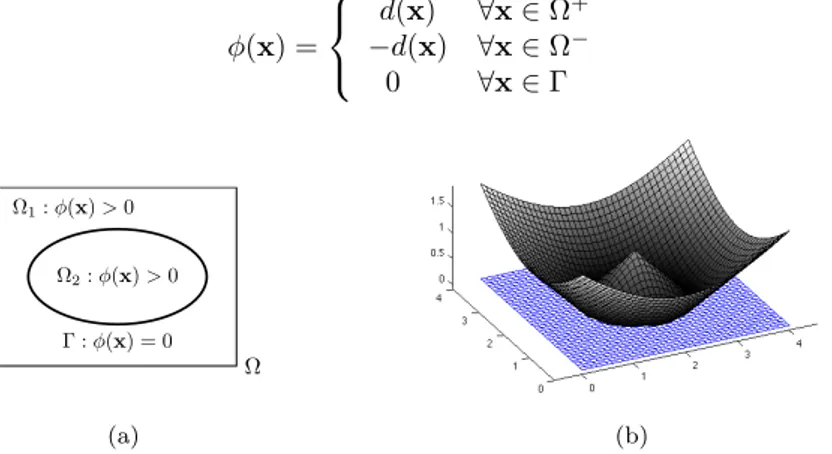
Different Level Set functions φ(x) can be used. Among those, the most popular one is the signed distance function. The distance function (Eq.(3)) associates a point x with the distance to the closest shape point xΓ.
φ(x) = d(x) = min
xΓ∈Ω
||x − xΓ|| (3)
The signed distance function (Eq.(4)) gives a sign to the distance value according to the location of the considered point x. φ(x) = d(x) ∀x ∈ Ω+ −d(x) ∀x ∈ Ω− 0 ∀x ∈ Γ (4) Ω Ω1: φ(x) > 0 Ω2: φ(x) > 0 Γ : φ(x) = 0 1 (a) (b)
Figure 1: Representing a unit circle with the distance function.
Ω Ω+: φ(x) > 0 Ω−: φ(x) < 0 Γ : φ(x) = 0 1 (a) (b)
Figure 2: Representing a unit circle with the signed distance function. 5.2 Level Set and XFEM
Working with FEM or XFEM, shape and boundaries of a structure are discretized on an associated mesh. Values of the Level Set function φiare computed on each mesh node. These discrete Level Set values are
then interpolated on the whole structure using the standard finite element shape functions. φh(x) =X
i
Ni(x) φi (5)
The Level Set description and extended finite element method can be advantageously combined. In fact XFEM uses special enrichment functions to represent particular solutions on some chosen elements, called enriched elements. Describing geometries with Level Sets eases the choice of these enriched elements. 6. eXtended Finite Element Method (XFEM)
Carrying out shape optimization using classical finite element method arises several problems. The stud-ied structure has to be meshed in a conform way. To track shape modifications, a new mesh has to be
generated for each optimization iteration. Extended finite element method circumvents these kinds of problems. It allows us to mesh the studied structure in a non conform way. Therefore shape changes don’t systematically come with remeshing.
6.1 Principle of XFEM
Extended finite element method allows to deal with the particular behavior of the structure near discon-tinuities, boundaries and interfaces... by adding special enriched shape functions to the finite element approximation (Eq.(6)). Enriched shape functions are build by multiplying standard finite element shape functions Ni(x) and particular enrichment functions ψ(x).
uh(x) =X i∈I Ni(x) ui | {z } FEM +X i∈I? Ni(x) ψ(x) ai | {z } Enrichment (6)
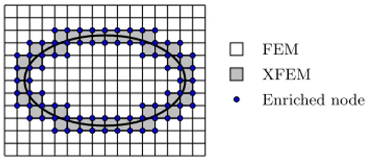
Enrichment is achieved locally, i.e. enriched shape functions are only added to the approximation when necessary. Level Set description will ease the task of choosing elements to be enriched because these will be cut by the iso-zero level φ(x) = 0.
FEM XFEM Enriched node
Figure 3: Choosing elements to be enriched in a structure. 6.2 Enrichment functions
There exist many different enrichment functions depending on which particular behavior of the structure to be represented. For weak discontinuities, such as interfaces... the abs-enrichment or the ridge function can be used. For strong discontinuities, such as cracks... the Heaviside function can be used.
x
ψ(x)
(a) The abs-enrichment
x
ψ(x)
(b) The ridge function
x ψ(x) (c) Heaviside 1st defini-tion x ψ(x) (d) Heaviside 2nd defini-tion
Figure 4: Enrichment functions in 1D.
In this work, we focus on two particular types of discontinuity: void-material interfaces and bimaterial interfaces. Modeling void-material interfaces, elements cut by the iso-zero Level Set must be enriched. In this case, additional degrees of freedom are not necessary. The Heaviside function is used and the displacement field is approximated as shown in Eq.(7).
uh(x) =X
i
Ni(x) H(x) ui (7)
where Ni(x) are the classical finite element shape functions, H(x) the Heaviside function and ui the
degrees of freedom associated to the classical finite element shape functions.
Dealing with bimaterial structures, the discontinuity modelized is an interface between two materials exhibiting different properties. Elements cut by the iso-zero Level Set must be enriched and additional degrees of freedom are introduced. The ridge function is used and the displacement field is approximated as shown in Eq.(8). uh(x) =X i Ni(x) ui+ X i Ni(x) g(x) ai (8) 3
where Ni(x) are the classical finite element shape functions, ui the degrees of freedom associated to the
classical finite element shape functions, g(x) = P
jNj(x) |φj| − |Nj(x) φj| the ridge function, φj the
nodal values of the Level Set function, ai the additional degrees of freedom.
6.3 Implementation of XFEM
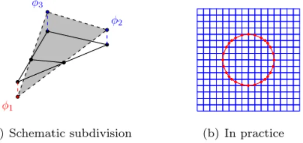
XFEM codes are not exactly similar to classical FEM codes. Among the differences, key ones are the subdivision and the integration of the enriched elements.
Each cut element must be divided in several subelements. The subdivision work is made easier by using Level Set description of geometries as shown in Fig.(5).
φ1
φ2 φ3
1
(a) Schematic subdivision
Student Version of MATLAB (b) In practice
Figure 5: Subdivision of enriched elements using Level Set description of geometries.
Integration can’t be performed as it was for classical finite elements. If it was the case, Gauss points used for the integration could be badly located or one could require a tremendous amount of Gauss points to capture the non linear behaviors. We could get subelements with several Gauss points and others with none. To avoid these problems, each subelement is mapped to a second parametric space (s, t). Gauss points are brought back from the second parametric space (s, t) to the first one (ξ, η) where classical Gauss integration is performed for each subelement as shown in Fig.(6).
x y 2 1 3 J1 ξ η 1 2 3 x x x J2 s t x x x 1
Figure 6: Dealing with integration of extended finite element. 7. Sensitivity analysis
A key part of the shape optimization process is the sensitivity analysis. Working with classical finite elements, the sensitivity analysis is a laborious task since every shape modification leads to remeshing. Coupling Level Set description and XFEM, the sensitivity analysis can be realized on a fixed mesh. De-sign variables z of the optimization problem are the Level Set parameters. They are perturbed and their influence on mechanical responses of the structure is measured.
7.1 Semi-analytical approach
The sensitivity analysis is carried out using a semi-analytical approach. Derivatives of the stiffness matrix K and the external force vector g with respect to Level Set parameters are computed through forward finite difference as shown in Eq.(9) and Eq.(10).
∂K ∂z ' K(z + δz) − K(z) δz (9) ∂g ∂z ' g(z + δz) − g(z) δz (10)
Then these derivatives are used to compute variations of different objective functions, such as compliance, displacements or stresses.
7.2 Implementation of the semi-analytical approach
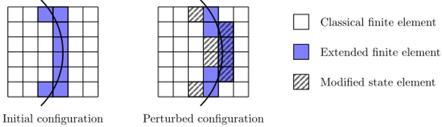
In practice, applying this semi-analytical method is not trivial. While perturbing the Level Set param-eters, the shape of the studied boundary or interface is modified. Some elements, initially uncut by the iso-zero Level Set, could be cut after perturbation of the parameters. Nodes of these elements should then be enriched, leading to additional degrees of freedom in the structure. For these elements, that change state from cut to uncut or from uncut to cut by the iso-zero Level Set as shown in Fig.(7), finite difference can not be performed. In the case of void-material interface, new degrees of freedom will be ignored introducing a small, but not significant, error in the sensitivities computation.
Initial configuration Perturbed configuration
Classical finite element Extended finite element Modified state element
1
Figure 7: Element state modifications after perturbation of the studied boundary. 8. Applications
The method, presented above, will be illustrated on several academic test cases. At first we revisit the classical problem of shape optimization of microstructures design investigated by Vigdergauz [4]. The analytical optimal shape of a single void inclusion can be recovered using numerical optimization in a very flexible way. Then the microstructural optimization is extended to tailor effective properties with the control of local responses at the microstructural scale.
9. Acknowledgements
The first author, Lise No¨el, would like to acknowledge the Belgian National Fund for Scientific research (F.R.S.-FNRS) for its support.
10. References
[1] O. Sigmund. Materials with prescribed constitutive parameters: An inverse homogenization problem. International Journal of Solids and Structures, 31(17):2313–2329, 1994.
[2] N. Moes, M. Cloirec, P. Cartraud, and J.-F. Remacle. A computational approach to handle complex microstructure geometries. Computer Methods in Applied Mechanics and Engineering, 192:3163– 3177, 2003.
[3] L. Van Miegroet and P. Duysinx. Stress concentration minimization of 2d filets using x-fem and Level Set description. Structural and Multidisciplinary Optimization, 33(4):425–438, 2007.
[4] S. Vigdergauz. The effective properties of a perforated elastic plate numerical optimization by genetic algorithm. International Journal of Solids and Structures, 38:8593–8616, 2001.