2014 — Macroblock level rate and distortion estimation applied to the computation of the Lagrange multiplier in H.264 compression

ÉCOLE DE TECHNOLOGIE SUPÉRIEURE UNIVERSITÉ DU QUÉBEC

THESIS PRESENTED TO

ÉCOLE DE TECHNOLOGIE SUPÉRIEURE

IN PARTIAL FULFILLEMENT OF THE REQUIREMENTS FOR THE MASTER DEGREE IN

INFORMATION TECHNOLOGY ENGINEERING M. Eng.

BY

Alexandru COTOROS PETRULIAN

MACROBLOCK LEVEL RATE AND DISTORTION ESTIMATION APPLIED TO THE COMPUTATION OF THE LAGRANGE MULTIPLIER IN H.264 COMPRESSION

MONTREAL, MARCH 17, 2014

© Copyright reserved

It is forbidden to reproduce, save or share the content of this document either in whole or in parts. The reader who wishes to print or save this document on any media must first get the permission of the author.

BOARD OF EXAMINERS

THIS THESIS HAS BEEN EVALUATED BY THE FOLLOWING BOARD OF EXAMINERS

Mr. Stéphane Coulombe, Thesis Supervisor

Département de génie logiciel et des TI at École de technologie supérieure

Mrs. Rita Noumeir, President of the Board of Examiners

Département de génie électrique at École de technologie supérieure

Mr. Christian Desrosiers, Member of the jury

Département de génie logiciel et des TI at École de technologie supérieure

THIS THESIS WAS PRENSENTED AND DEFENDED

IN THE PRESENCE OF A BOARD OF EXAMINERS AND PUBLIC ON FEBRUARY 13, 2014

ACKNOWLEDGMENTS

I would like to thank my advisor, Professor Stéphane Coulombe, for the chance to perform this research at Vantrix Industrial Research Chair in Video Optimization Laboratory, and for the opportunity to learn and work on such a great research project under his invaluable supervision. I would also like to express my deepest appreciation for his mentorship, encouragement and for sharing his great professional experience throughout my Master’s program.

I would like to thank him and the company Vantrix, not only for providing the scholarship which allowed me to pursue this research, but also for giving me the opportunity to attend the group meetings and collaborate with engineers and researchers in the field of video processing.

I would like to thank the board of examiners that gave generously of their time for reviewing this thesis and for their participation in my defense examination.

I would also like to thank Ms. Deepa Padmanabhan and Nick Desjardins for the important contribution they brought to the validation of this project.

Special thanks to anyone who has taken time to take a look, make suggestions and proofread this thesis.

ESTIMATION DU DÉBIT ET DE LA DISTORSION AU NIVEAU DU MACROBLOC APPLIQUÉE AU CALCUL DU MULTIPLICATEUR DE

LAGRANGE EN COMPRESSION AVEC LA NORME H.264 Alexandru COTOROS PETRULIAN

RÉSUMÉ

La valeur optimale du multiplicateur de Lagrange (

λ

), un facteur de compromis entre le débit obtenu et la distorsion mesurée lors de la compression d’un signal, est un problème fondamental de la théorie de la débit-distorsion et particulièrement de la compression vidéo.

Le standard H.264 ne spécifie pas comment déterminer la combinaison optimale des valeurs des paramètres de quantification (QP) et des choix de codage (vecteurs de mouvement, choix de mode). Actuellement, le processus d’encodage est encore dépendant de la valeur statique du multiplicateur de Lagrange, dont une dépendance exponentielle du QP est adoptée par la communauté scientifique, mais qui ne peut pas accommoder la diversité des vidéos. La détermination efficace de sa valeur optimale reste encore un défi à relever et un sujet de recherche d’actualité.

Dans la présente recherche, nous proposons un nouvel algorithme qui adapte de façon dynamique le multiplicateur de Lagrange en fonction des caractéristiques de la vidéo d’entrée en utilisant la distribution des résidus transformés au niveau du macrobloc. Le but recherché est d’augmenter la performance de codage de l’espace débit-distorsion.

Nous appliquons plusieurs modèles aux coefficients résiduels transformés (Laplace, Gaussien, densité de probabilité générique) au niveau du macrobloc pour estimer le débit et la distorsion et étudier dans quelle mesure ils correspondent aux vraies valeurs. Nous analysons ensuite les bénéfices et désavantages de quelques modèles simples (Laplace et un mélange de Laplace et Gaussien) du point de vue du gain en compression et de l’amélioration visuelle en rapport avec le code de référence du standard H.264 (amélioration débit-distorsion).

VIII

Plutôt que de calculer le multiplicateur de Lagrange basé sur un seul modèle appliqué sur toute la trame, comme proposé dans l’état de l’art, nous le calculons basé sur des modèles appliqués au niveau du macroblock. Le nouvel algorithme estime, à partir de la distribution des résidus transformés du macrobloc, le débit et la distorsion de chacun, pour ensuite combiner la contribution de chacun pour calculer multiplicateur de Lagrange de la trame.

Les expériences sur des types variés de vidéos ont démontré que la distorsion calculée au niveau du macrobloc est proche de la distorsion réelle offerte par le logiciel de compression vidéo de référence pour la plupart des séquences vidéo testées, mais un modèle fiable pour le débit est encore recherché particulièrement à très bas débit. Néanmoins, les résultats de compression de diverses séquences vidéo montrent que la méthode proposée performe beaucoup mieux que le Joint Model du standard H.264 et un peu mieux que l’état de l’art.

MACROBLOCK LEVEL RATE AND DISTORTION ESTIMATION APPLIED TO THE COMPUTATION OF THE LAGRANGE MULTIPLIER IN H.264

COMPRESSION

Alexandru COTOROS PETRULIAN ABSTRACT

The optimal value of Lagrange multiplier, a trade-off factor between the conveyed rate and distortion measured at the signal reconstruction has been a fundamental problem of rate distortion theory and video compression in particular.

The H.264 standard does not specify how to determine the optimal combination of the quantization parameter (QP) values and encoding choices (motion vectors, mode decision). So far, the encoding process is still subject to the static value of Lagrange multiplier, having an exponential dependence on QP as adopted by the scientific community. However, this static value cannot accommodate the diversity of video sequences. Determining its optimal value is still a challenge for current research.

In this thesis, we propose a novel algorithm that dynamically adapts the Lagrange multiplier to the video input by using the distribution of the transformed residuals at the macroblock level, expected to result in an improved compression performance in the rate-distortion space.

We apply several models to the transformed residuals (Laplace, Gaussian, generic probability density function) at the macroblock level to estimate the rate and distortion, and study how well they fit the actual values. We then analyze the benefits and drawbacks of a few simple models (Laplace and a mixture of Laplace and Gaussian) from the standpoint of acquired compression gain versus visual improvement in connection to the H.264 standard.

Rather than computing the Lagrange multiplier based on a model applied to the whole frame, as proposed in the state-of-the-art, we compute it based on models applied at the macroblock

X

level. The new algorithm estimates, from the macroblock’s transformed residuals, its rate and distortion and then combines the contribution of each to compute the frame’s Lagrange multiplier.

The experiments on various types of videos showed that the distortion calculated at the macroblock level approaches the real one delivered by the reference software for most sequences tested, although a reliable rate model is still lacking especially at low bit rate. Nevertheless, the results obtained from compressing various video sequences show that the proposed method performs significantly better than the H.264 Joint Model and is slightly better than state-of-the-art methods.

TABLE OF CONTENTS

INTRODUCTION ...1

AN OVERVIEW OF VIDEO COMPRESSION ...5

CHAPTER 1 1.1 Basic concepts in the H.264 standard ...5

1.1.1 Prediction ... 5

1.1.2 Residual coefficients ... 10

1.1.3 Transform and quantization ... 11

1.1.4 Mode decision and the macroblock encoding ... 14

1.1.5 The bit cost of coding a macroblock ... 15

1.1.6 Entropy encoding ... 15

1.1.7 Visual quality and encoding performance indexes ... 16

1.2 Rate distortion optimization in H.264 ...17

1.2.1 Cost function ... 18

1.2.2 Optimal Lagrange multiplier ... 20

1.2.3 Lagrange multiplier for high rate encoding ... 22

1.3 General block diagram of video compression ...23

CHAPTER 2 LITERATURE OVERVIEW ...27

2.1 Lagrange multiplier selection ...27

2.1.1 Laplace distribution-based approach for inter-frame coding ... 29

2.1.2 Laplace distribution-based approach for intra-frame coding ... 35

2.1.3 SSIM-based approach ... 36

2.2 Types of distribution of the residual transformed coefficients ...41

2.2.1 Gaussian model ... 43

2.2.2 Laplace model ... 43

2.2.3 Generalized Gauss model ... 45

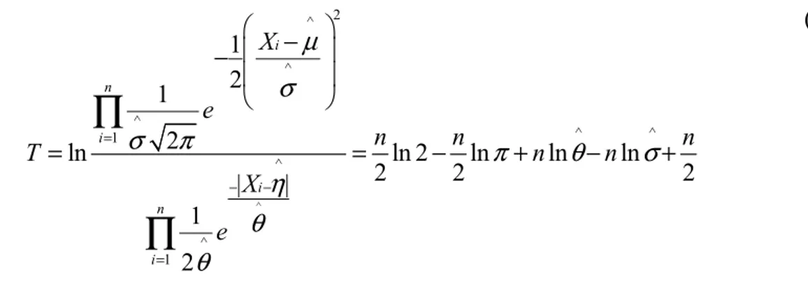
2.2.4 Proof test ... 47

2.2.5 Generic model based on numerical integration ... 48

RATE DISTORTION ESTIMATION ASSOCIATED TO LAPLACE, CHAPTER 3 GAUSS, GENERALIZED GAUSS, AND NUMERICAL INTEGRATION COEFFICIENT MODELS ...51

3.1 General Rate-Distortion equations ...51

3.2 Rate-Distortion equations associated to Laplace model ...52

3.2.1 Rate equation associated to Laplace model ... 53

3.2.2 Distortion equation associated to Laplace model ... 53

3.3 Rate-Distortion equations associated to Gaussian model ...54

3.3.1 Rate equation associated to Gaussian model ... 54

3.3.2 Distortion equation associated to Gaussian model ... 55

3.4 Rate-Distortion equations associated to generalized Gaussian model ...56

XII

3.4.2 Distortion equation associated to generalized Gaussian model ... 56

3.5 Rate-Distortion equations associated to generic model ...57

3.5.1 Rate equation associated to generic model ... 57

3.5.2 Distortion equation associated to generic model ... 58

3.6 Comparison of the distortion models at different QPs ...58

3.7 Comparison of entropy models at different QPs...61

MACROBLOCK LEVEL ADAPTIVE LAGRANGE MULTIPLIER CHAPTER 4 COMPUTATION ...65

4.1 Motivation ...65

4.2 RDO using frame level Laplace distribution based Lagrange multiplier ...68

4.2.1 Analysis of multiple coding units having Laplace distribution ... 69

4.2.2 Macroblock level processing ... 76

4.3 Macroblock level adaptive Lagrangian multiplier computation ...79

4.3.1 The optimal Lagrange multiplier as a function of QP for Laplace distribution based model ... 79

4.3.2 The optimal Lagrange multiplier as a function of QP for Gauss distribution based model ... 81

4.3.3 The optimal Lagrange multiplier for generic distribution based model ... 81

4.4 Rate distortion optimization using the macroblock level adaptive Lagrange multiplier computation applied to H.264 compression...83

4.5 Summary of the methodology used for experiments ...85

EXPERIMENTAL RESULTS ...87

CHAPTER 5 5.1 Experimental setup...87

5.2 Model parameters estimation at the macroblock level ...89

5.3 H.264 rate and distortion estimation at macroblock level ...94

5.4 H.264 RDO using frame level adaptive at the region level ...99

CONCLUSION ………..103

LIST OF TABLES

Page

Table 1.1 PSNR to MOS mapping. ...17

Table 1.2 Lagrange multiplier with high rate assumption ...22

Table 2.1 Laplace and Gauss distribution - parameters comparison ...45

Table 5.1 Consolidated statistics of MB models applied to sequence container_cif ...95

Table 5.2 Consolidated statistics of MB models applied to sequence container_qcif ...95

Table 5.3 The new approach applied to sequence container_qcif ...97

Table 5.4 The new approach applied to the sequence silent_qcif.yuv ...98

Table 5.5 Comparison between coding with Laplace at the frame level (FrameLM) and the new approach with respect to the standard implementation of JM ...102

LIST OF FIGURES

Page

Figure 1.1 4x4 intra prediction modes...6

Figure 1.2 Intra 16x16 prediction modes. ...7

Figure 1.3 Macroblock/sub-macroblock partitions for interframe coding. ...8

Figure 1.4 The forward transform and quantization. ...11

Figure 1.5 Inverse quantization and transform. ...13

Figure 1.6 DZ + UTSQ/NURQ scheme. ...13

Figure 1.7 Available prediction modes. ...14

Figure 1.8 H.264 encoder block diagram. ...24

Figure 2.1 RD curves, from (Li and others, 2009) ...34

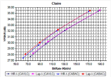
Figure 2.2 RD curves for Claire_qcif.yuv, from (Li, Oertel and Kaup, 2007) ...35

Figure 2.3 RD curves for the SSIM approach, from (Wang and others, 2012) ...41

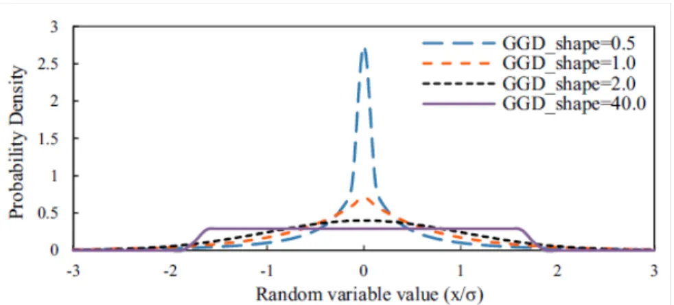
Figure 2.4 Zero-mean generalized Gaussian distribution. ...45

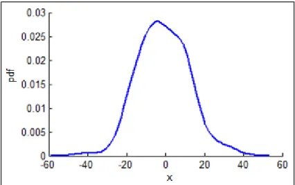
Figure 2.5 The real distribution of transform residuals; seq. Bus (QCIF), frame #6(P) ...48

Figure 2.6 The real distribution of transform residuals, frame #6(P), MB (5, 8), ...49

Figure 2.7 The real distribution of transform residuals, frame #6(P), MB (3, 7), ...49

Figure 3.1 The distortion calculated with: a) Laplace pdf, b) Gauss pdf ...59

Figure 3.2 The distortion calculated with generalized Gauss: a)

_α

₌1(Laplace), b)

_α

₌2 (Gauss) ...60

Figure 3.3 The entropy (bits/sample) calculated with: a) Laplace pdf and b) Gauss pdf .62 Figure 3.4 The entropy (bits/sample) calculated with GGD: a)

α

=1(Laplace) and b) 2

α

= (Gauss) ...63

XVI

Figure 4.2 Histogram of MB level Laplace parameters for frame 10 of QCIF sequences

Foreman and Container encoded at QP = 32 ...68

Figure 4.3 Histogram of MB level Laplace parameters for frame 10 of QCIF sequences Foreman and Container encoded at QP = 40 ...69

Figure 4.4 Laplace distributions of coding units with Λ1 = 0.15, Λ2 = 0.25, and Λ3 = 0.25 and frame level approximation, for Foreman_qcif.yuv ...71

Figure 4.5 R-D curve of MCU and frame level approximation for MCU comprised of ..72

Figure 4.6 Lagrange multiplier for MCU and frame level approximation for MCU comprised ofΛ1 = 0.15, Λ2 = 0.25, and Λ3 = 0.25, for Foreman_qcif.yuv ..73

Figure 4.7 Laplace distributions of coding units and frame level approximation ...74

Figure 4.8 R-D curve of MCU and frame level approximation for MCU comprised of ..75

Figure 4.9 Lagrange multiplier for MCU and frame level approximation for MCU comprised of Λ1 = 0.25, Λ2 = 0.35, Λ3 = 0.45, Λ4 = 0.55, and Λ5 = 0.65, for Container_qcif.yuv ...75

Figure 4.10 Lagrange multiplier: a) Laplace-based; b) GGD-based (_{α =}1) ...80

Figure 4.11 Lagrange multiplier: a) Gauss-based; b) GGD-based (_{α =}2). ...82

Figure 4.12 Operational RD and RD model curves. ...83

Figure 4.13 Block diagram of one step and one frame delay encoding. ...86

Figure 5.1 Distribution of frame transformed residuals (container, frame 2(P)), ...91

Figure 5.2 Container_qcif.yuv, frame 2(P), QP = 20, rendered with mixed (Gauss and Laplace) model ...92

Figure 5.3 Container_qcif.yuv frame 2(P) QP = 36, rendered with mixed (Gauss and Laplace) model ...93

Figure 5.4 PSNR vs. bitrate and

λ

mcu vs. QP of container_cif.yuv ...100

LIST OF ABBREVIATIONS AC Non-zero frequency (of transformed coefficients) AVC Advanced Video Coding

CABAC Context-based Adaptive Binary Arithmetic Coding CAVLC Context-based Adaptive Variable-Length Coding CIF Common Intermediate Format

DC Zero frequency (of transformed coefficients) DCT forward Discrete Cosine Transform

DPB Decoded Picture Buffer

EPZS Enhanced Predictive Zonal Search

FPel Motion compensation by interpolation with integer-pixel (Full Pel) accuracy GGD Generalized Gauss Distribution

HPel Motion compensation using interpolation with half-pixel accuracy HVS Human Visual System

i.i.d. independent and identically distributed (random variable, process) IDCT Inverse Discrete Cosine Transform

JM Joint Model (reference software) MB Macroblock

MC Motion Compensation

MCU Multiple Coding Units

MD Mode Decision

ME Motion Estimation

MOS Mean Opinion Score MSE Mean Squared Error

MV Motion Vector

pdf probability density function QCIF Quarter Common Intermediate Format

QP Quantization Parameter

QPel Motion compensation using interpolation with quarter-pixel accuracy RD Rate-Distortion

XVIII

RDO Rate-Distortion Optimization SAD Sum of Absolute Differences

SSE Sum of Squared Errors SSIM Structural Similarity Index

LIST OF SYMBOLS

mcu

λ

Lagrange multiplier using the MCU approach

HR

λ

Lagrange multiplier determined with high rate approximation

MODE

λ

Lagrange multiplier for the mode decision stage

MOTION

λ

Lagrange multiplier for the motion estimation stage

λ

Lagrange multiplier

Λ Laplace parameter

η

location (expected value of Laplace distribution)

θ

scale

μ

mean value (expected value of Gauss distribution)

σ standard deviation

γ

rounding offset of the quantization step

α shape parameter describing the exponential rate of decay (GGD)

β

standard deviation (GGD) D distortion

J cost function

Q quantizer step size

R bit rate

INTRODUCTION Context

This research endeavors to find the highest quality of the video that would allow exporting a reasonably smaller amount of bits, so that the overall coding gain is superior to the actual one.

Problem statement

The fundamental problem in video compression is to obtain the best trade-off between the conveyed rate and the perceived distortion of the reconstructed video. The H.264 standard has only the syntax standardized, but it does not specify how the optimal values, e.g. the Lagrange multiplier, may be obtained, nor the best encoder configuration or coding decisions. Rate-distortion optimization is originally posed as a constrained problem of finding the minimum distortion under a rate constraint. For simplicity, this problem is converted into an unconstrained optimization one using a Lagrangian method in which the Lagrange multiplier needs to be carefully selected. The rate, as a byproduct of distortion calculation and Lagrange multiplier determination, is not always well-calculated and it is a challenge to find its best value in combination with the other two. On the other hand, the Lagrange multiplier depends on the video source features, while the distortion should be calculated with the help of a modern visual quality metric, based on the human visual system (HVS). Despite these difficulties, it is believed that there is enough room for significant improvement of the bit allocation with video quality improvement, for any type of video content. It is supported by the huge amount of research in this direction.

In the end, the problem of finding the optimal value of Lagrange multiplier that would determine balanced values of the pair (distortion, rate) from the standpoint of video quality and bit allocation is fundamental in these respects. Huge investments have been injected in the related industries (entertainment, communication, social media, business, defense, health,

2

video surveillance, traffic management) that made video so widespread and continually growing expressing the need to visually communicate at higher resolutions. YouTube, the largest and most popular user-generated video-hosting site, has demonstrated the insatiable and widespread demand for video content. In 2011, the site reported one trillion video viewings in total - an average of 140 viewings per capita, on the entire world population; and reports that approximately four billion hours of video are watched per month (Atkinson, 2012). These staggering figures apply for just one site - and the demand is ever-growing. Indeed, many broadcasting corporations have responded to the increasingly web-based desire for content and have made television shows available for streaming off their individual online sites (Barker, 2011). Ever since the slow but sure decline of video rental businesses like Blockbuster (Carr, 2010), which loaned popular titles on physical disks, other companies have taken up the torch of modern video subscription services. Netflix has seen its consumer base grow to 30 million subscribers in 2012 (Etherington, 2012), and other providers such as iTunes (Yarow, 2013) and Amazon Video (Stone, 2013) have been growing steadily as well.

One of the most important factors in the exponential growth of video demand is the combination of social integration with increasingly more popular mobile devices. YouTube reports 500 years of video being watched every day just through links on social platforms like Facebook, and 700 videos being shared every minute on Twitter (Atkinson, 2012). Bandwidth demand for mobile video has exploded since the growth of ever-more capable portable devices, especially in the smartphone and tablet sector (Kovach, 2013). The adoption of and desire for high-quality video has been a leading force in the hunger for greater bandwidth capacity, speed and reliability, in the form of residential, corporate and cellular data availability. Especially in the case of the latter, telecommunications companies have invested billions of dollars into emerging technologies, like long-term evolution networks that ensure faster and more reliable data transfers, while increasing bandwidth capacity. The mass-adoption of these technologies by consumers will ensure their long-term sustainability, although predictably, speeds are bound to suffer as more traffic is introduced. The heaviest burden on these networks is undoubtedly the transfer of video content – whether it is video conferencing over services like Microsoft’s Skype or Apple’s Face Time, watching

television (TV) shows on-the-go, or uploading home videos straight from mobile devices. Clearly, there is an increasing demand to communicate and share information today that is only the beginning of the years to come.

Short literature overview

The Lagrange multiplier

λ

, the balancing factor between rate and distortion in rate-distortion theory, evolved with the versions of the video standards. While H.263 used an expression depending on the square of the quantization parameter (QP) only, H.264/AVC (Advanced Video Coding) promoted a value that grows exponentially with QP, but both expressions of

λ

are static, regardless of the sequence. The state-of-the-art approach (Li and others, 2009) has set the trend of using variable Lagrange multipliers, adaptive with the statistical properties of the video content, which resulted in a different value of

λ

for each frame. This method allows getting compression improvements, especially on slow paced videos. New visual quality metrics closer to HVS, such as the structural similarity index (SSIM) have emerged, replacing the sum of squared errors (SSE) and giving a boost to

λ

calculated per frame and adjusted at the macroblock level as (Wang and others, 2012) propose.

The thesis is organized as follows: Chapter 1 centers on basic concepts related to video compression and rate-distortion theory whereas chapter 2 presents the state-of-the-art approaches and various types of distributions for the transformed residual coefficients. In chapter 3, the focus is on the Laplace and Gauss equations for rate and distortion, while the fourth one outlines the methods to determine the Lagrange multiplier at the macroblock level. Chapter 5 presents the experimental results. Chapter 6 concludes this thesis.

Contributions

This work proposes a new algorithm to dynamically adapt the Lagrange multipliers based on the distribution of transform residuals at the macroblock level, whose purpose is to improve the performance in terms of rate-distortion.

4

We study the estimation of rate and distortion functions, at the macroblock level, using various probability distribution functions for the transformed residuals, choosing from Laplace, Gauss, generalized Gauss and a generic, numerically computed, probability density function (pdf). We then conceive an algorithm for computing the Lagrange multiplier based on each macroblock’s rate and distortion functions. This permits selecting the most appropriate pdf per macroblock instead of assuming that a single distribution applies to the whole frame. This permits to estimate adaptively the most appropriate

λ

for each frame based on macroblock’s statistics and use it both at the motion compensation and mode decision stages of the compression.

CHAPTER 1

AN OVERVIEW OF VIDEO COMPRESSION

In this chapter, the fundamental notions and basic functionality of the H.264 standard are presented, followed by a description of the Lagrangian multiplier technique, as an efficient way to solve the rate distortion optimization problem. Finally, a block diagram summarizes the way the rate distortion optimization mechanism integrates with the main coding flow and how their functional relationship may be exploited for the benefit of the video compression.

1.1 Basic concepts in the H.264 standard

H.264/MPEG-4 Part 10 AVC (Advanced Video Coding) is the standard for video compression that is the most widespread. It is based on concepts such as prediction, motion estimation, motion compensation, mode decision, transformation, quantization, entropy encoding, deblocking, visual quality, that are described next.

1.1.1 Prediction

The compression performance of the encoder depends on the efficiency of the prediction methods. In order to create a slim residual, as scarce as possible of non-zero data, an accurate prediction is detected and extracted from the original macroblock. Thus, the best match of the current block, chosen inside one of the designated reference frames, is chosen so as to minimize the necessary bits to encode the motion vectors.

The prediction block found is further used to generate the residual transformed coefficients. In the case of the intra prediction, the best match of an I-type macroblock is searched by using the adjacent and previously coded blocks in the same slice (frame). In this way, one exploits the existing spatial correlation between the current block to be encoded and its

6

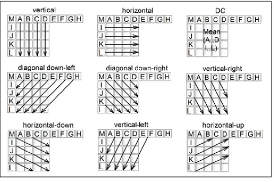
neighbors. The best intra prediction is searched at different block sizes. In AVC there are 9 possible prediction modes for a 4x4 and 8x8 luma blocks as illustrated in Figure 1.1.

For a luma macroblock or chroma block there are four possible intra prediction modes in AVC as illustrated in Figure 1.2. In order to increase the coding efficiency, the most probable prediction mode is calculated as the starting point before entering the search phase.

Since the nearest samples in the signal are not fully independent and identically distributed (i.i.d.), high correlations between them exist in the temporal domain, i.e. between temporally adjacent frames. The correlation degree increases with the sampling rate.

Figure 1.1 4x4 intra prediction modes. Adapted from (Richardson, 2010)

Inter prediction comes into play, taking advantage of the previously reconstructed frames, available in the decoded picture buffer (DPB), thus motion compensating the encoding with the offset between the original and its prediction. The macroblock/block estimate is searched in a region, usually a 32 pixel square, centered on the original macroblock.

The current macroblock can be predicted as predicted (P) type (also called inter) when the samples chosen as reference are selected from the list of past encoded frames or bidirectional (B) type, in which case, the prediction is based on samples in the list of past and respectively the list of future encoded frames, from the standpoint of displaying order.

Figure 1.2 Intra 16x16 prediction modes. Adapted from (Richardson, 2010)

A (P/B) Skip mode, which is only permitted in P/B slices, occurs when no data – MVs (motion vectors) differences and transformed residual coefficients - are transmitted to the decoder. Yet, the macroblock data is reconstructed at the decoder, through interpolation of the previously coded data, using the motion compensated prediction with a MV derived from previously sent vectors of a single reference frame in the case of P-Skip mode, or from two adjacent reference frames in the case of B-Skip Direct mode.

When the motion in the scene is so complex that the macroblock size would be too big to observe it in detail, the macroblock is divided into partitions (8x16, 16x8, and 8x8) and further sub-partitions of the block 8x8 (4x8, 8x4 and 4x4) as illustrated in Figure 1.3. Though the partitioning has the drawback of increasing the amount of motion vectors to transmit, looking for smaller partitions (8x8, 4x8, 8x4, and 4x4) has the benefit of decreasing the energy of the signal difference between the original and the best match. The optimal prediction of a macroblock (block) is always accompanied by its associated motion vector.

8

Figure 1.3 Macroblock/sub-macroblock partitions for interframe coding. Adapted from (Richardson, 2010)

The motion vector refers to the offset between the positions of the current partition and its best prediction in the reference frame(s). It can point to integer, half or quarter pixel positions in the luma component of the reference picture, depending on the pixel accuracy with which the search is performed. The half-pixel luma samples are generated using a 6 tap finite impulse response (FIR) filter applied to integer-pixel samples in the reference frame, while the quarter-pixel samples are inferred through linear interpolation between adjacent half pixel samples. Alternately, in order to increase the motion accuracy at 4:2:0 resolution, the quarter pixel positions are calculated for chroma samples using a 4 tap FIR to interpolate between the neighboring integer and half pixel positions.

The motion estimation process, available for inter-prediction only, defines the space of pair solutions (predicted regioni, MVi) that are searched upon. The best prediction does not necessarily involve the minimum effort to encode its motion vector (MV). Although small (sub) partitions offer the best estimate, encoding their motion vectors can incur a significant number of bits. The spatial and temporal correlation between nearby partitions is often found at the level of their motion vectors; hence the motion vector of a block can be predicted from those associated to the previously coded blocks. The motion vectors prediction applies spatially, by considering the median of the surrounding blocks MVs. What is encoded in the macroblock’s header is the difference between the current MV and the predicted motion vector MVp.

The outcome of the prediction phase for the current block is the estimated block and the associated motion vector that is used to motion compensate the encoded macroblock with respect to reference frame(s). Only the motion vectors differences are encoded in the bitstream, namely in the macroblock header, while the prediction is further used to shape the coefficients of the residual block.

Among the most efficient methods of finding the best prediction are the zonal search algorithms represented by PMVFAST (Tourapis, Au and Liou, 2001) and its extension, Enhanced Predictive Zonal Search or EPZS for short (Tourapis, 2002). PMVFAST enhances the speed and video quality by considering the following as initial predictors: the motion vectors of spatially adjacent blocks in the current frame, the (0, 0) motion vector, the median predictor, and the motion vector of the collocated block in the previous frame, all, as a matter of temporal domain correlation. It introduces reliable early-stopping criteria, at any check-point, based on correlations between adjacent blocks, though fixed thresholds are used to compare with the sum of absolute differences (SAD) values.

The highly efficient EPZS algorithm, improves upon PMVFAST by considering at prediction stage several highly likely predictors, based on multi-stage checking pattern. Key to its performance is the fact that the MVs of the current block can be highly correlated with the MVs of the spatially and temporally adjacent blocks and the introduction of the accelerator MV, to model the variable speed movement of the collocated block with respect to the previous two encoded frames. The current block can also be highly correlated with the adjacent blocks to the collocated block in the previous frame. The effect of these last predictors translates into decreasing entropy of the differences between EPZS MVs compared to PMVFAST MVs.

SAD, the distortion measure between the current frame

I

t and i-th previously encoded frame t i

I

− , displaced by MV with the components (vx, vy),

, , 1 ( , )x y M N_{m n} | (t , ) t i( x , y ) | SAD v v =



₌ I x m y n+ + −I₋ x v+ +m y v+ +n where M N, ∈{4,8,16} (1.1)

10

is compared to the thresholds that are adaptively calculated in the case of EPZS. Simplified search patterns, square or diamond of order one proved beneficial, significantly reducing the number of checking points and algorithm complexity.

The result of EPZS is a significant reduction of bits necessary to encode the MVs.

1.1.2 Residual coefficients

The prediction stage is lossless and partially removes redundancy by extracting the best matching estimation from the current macroblock (partition/sub-partition). The process of motion compensation takes into account the difference between their positions in terms of motion vector differences (MVD). The more precise the prediction is, the less energy in the residual remains, and the data becomes easier to compress to lesser bits. The residuals, as a difference between the original and predicted signals, contain much less energy than either component, so it requires fewer amounts of bits to be sent to the decoder.

As a matter of fact, since the best mode decision depends on finding the most suitable Lagrange multiplier to encode the macroblock, modeling the residuals has become a central problem in rate-distortion optimization (RDO).

Although the majority of natural phenomena and processes statistically behave in the Gaussian way, the residuals in video compression do not quite follow the same path. Similar to audio signals compression, the residuals should behave according to Laplace probability distribution only. In reality, as will be shown in chapter 4, at smaller QP, almost every sequence contains a percentage of Gaussian-distributed residual coefficients, and there is a tendency of macroblock residuals’ shape to morph from Laplace to Gauss distribution, when QP decreases.

The central problem of process modeling from the standpoint of macroblock distribution of residuals has been to determine the suitable kind of probability density function (pdf), by adequately evaluating its correctness according to the existing criteria of goodness of fit. Further, using several mathematical models of distortion and entropy, based on distribution of residuals, one can estimate better expressions for Lagrange multipliers.

1.1.3 Transform and quantization

The purpose of DCT is to further de-correlate, compact and translate the residual data into the frequency space, represented by the DC(zero frequency)/AC(non-zero frequency) transformed coefficients. In H.264, non-unitary and signal independent core matrices are defined for the stages of forward and inverse transforms, respectively of a 4x4 block:

4 4 1 1 1 1 2 1 1 2 1 1 1 1 1 2 2 1 f x C    _{− −}    =_{ } − −  _{− −}    4 4 1 1 1 1 1 1/ 2 1/ 2 1 1 1 1 1 1/ 2 1 1 1/ 2 i x C    _{− −}    =_{ } − −  _{− −}    (1.2)

Alternatively, the transforms Cf8x8 and Ci8x8 for 8x8 blocks processing exist.

The purpose of the transform is to decorrelate the input signal X from the productC X.C_f4. _f4T. Since the forward transform is not perfectly unitary, a diagonal matrix is hard to obtain, yet, beneficial is the fact that the signal energy is compacted in as little coefficients as possible.

Figure 1.4 The forward transform and quantization. Adapted from (Richardson, 2010)

12

At the end of the forward transform illustrated in Figure 1.4, the energy gets redistributed and concentrated into a smaller number of coefficients which makes it easier for entropy encoding. Although the product of orthogonal matrices for forward (Cf4x4) and inverse (Ci4x4) transform, even normalized, is not perfectly equal to unit matrix, their elements were intentionally multiplied/rounded to get a minimal set

{ 1, 2, 1 2}

± ± ±

of values that make the transform easily implementable, by using only additions and left/right bit shifts. This way one can avoid overwhelming floating point multiplication.

Due to the reversibility of the integer DCT, whose inverse matrix can be obtained through the transposing of the normalized core transform (unitary), the overall forward/inverse transform is lossless as well, as is the prediction stage.

In the case of 16x16 intra coded luma blocks and all-dimensions chroma blocks, the DC coefficients are further de-correlated through a DC 4x4 Hadamard transform. In the H.264/AVC standard, the transform and quantization phases overlap in order to minimize the computational effort that would otherwise be overwhelming for the processing unit(s) had they been performed separately.

In the intra-frame coding, DCT is applied to the macroblocks pertaining to the frame itself, while in inter-frame compression its input is defined as the difference between the current block and its prediction.

In addition, a normalization step, necessary to orthonormalize the core integer transform, is integrated with the quantization phase in order to reduce the number of multiplications. Up to this point, taking advantage of the spatial and temporal redundancy and de-correlating the signal, the prediction and transform stages are deemed as lossless steps.

The quantization process is the only lossy phase in the encoder, accounting for the trade-off between the compression performance and the perceived visual quality.

Figure 1.5 Inverse quantization and transform. Adapted from (Richardson, 2010)

At the end of the re-scaling and inverse transform illustrated in Figure 1.5 the reconstructed macroblock that emerges can be compared against the original one in order to assess the distortion.

While from the energy compaction standpoint, the Karhunen–Loève transform (KLT) is the best method. Its transformation matrix depends on the input signal statistics and lacks computational speed compared with the discrete cosine transform (DCT).

The quantization seen as a down scaling/re-scaling process of signal discretization /reconstruction is built on the linear scalar scheme containing the dead zone (DZ), an uniform threshold scalar quantization (UTSQ), and a nearly uniform reconstruction quantization (NURQ) as described in (Sun and others, 2013a) and (Wang, Yu and He, 2011). The rounding offsets (z, f) domain of the forward quantization and reconstruction, illustrated in Figure 1.6, are determined as:

(0.5 1)

z

_∈

_

,

f

∈ 

(0 0.5)

under the linear constraint

z f c

− =

,

c

∈

(0.5 1)

_

(1.3) with optimal values for intra (z = 2/3) and inter (z =5/6) coding.

Figure 1.6 DZ + UTSQ/NURQ scheme. Adapted from (Sun and others, 2013a)

14

A non-linear quantizer would appropriately reduce the amplitude of the transformed data, but would have to adaptively configure the threshold parameters (z, f), based on the density of the transformed signal’s pdf.

1.1.4 Mode decision and the macroblock encoding

Mode selection is the process of determining the best block partitions to encode a macroblock. It is governed by the RDO process, as presented in pseudo code in (Richardson, 2010) which takes into account the available modes shown in Figure 1.7.

For every macroblock

For every available coding mode m

Code the macroblock residual through DCT and quantization using the specific MVs for that mode m

Calculate R, the number of bits required to code the macroblock Reconstruct the macroblock through inverse quantization and IDCT Calculate D, the distortion between the original and decoded macroblock Calculate the mode costJMODE, with appropriate choice of Lagrange multiplier

end

Choose the mode that gives the minimum JMODE

End

The calculation of the mode cost JMODE was presented in section 1.2.1.

Figure 1.7 Available prediction modes. Adapted from (Richardson, 2010)

1.1.5 The bit cost of coding a macroblock

During the mode decision stage, when various modes are tested, the final decision is made when the minimum is attained by the cost functionJMODE. The number of bits necessary to

encode with the best mode is given in principal by two components (Richardson, 2010):

- The header bits, which contain the macroblock mode (I/intra, P/B inter coded), the prediction parameters (the entry (es) in the reference list(s), motion vectors differences for P/B macroblock, the search accuracy: full pel, (FPel), half pel (HPel), quarter pel (QPel).

- The transform coefficients bits as the bits necessary to encode the quantized transformed coefficients, CBP, QP, optimal mode.

1.1.6 Entropy encoding

The entropy coding is the last lossless stage of reducing the video information redundancy. The quantized coefficients are reordered through a zigzag scan to group together the non-zero (DC) values at the beginning of the run-length encoding, followed by the higher frequencies (AC) coefficients, most of them being runs of zeroes.

CAVLC (Context-based Adaptive Variable-Length Coding) maps the coefficients to a series of variable length codewords, using Huffman codes, where frequently-occurring symbols are represented with short variable-length code (VLC) (Richardson, 2010). It uses a context adaptive scheme based on several VLC look-up tables containing the updated statistics of the symbols to encode.

Unlike CAVLC, whose drawback is the assignment of an integral number of bits for each symbol, CABAC (Context-based Adaptive Binary Arithmetic Coding) encodes the whole message by mapping it to a subunit number. It uses context models (probability tables) and binarization schemes that feed the arithmetic coding engine with the necessary updated statistics of the symbols thus eliminating the multiplications operations. CABAC, though

16

slower than CAVLC, achieves a better compression by allowing fractional number of bits to represent a symbol, thus approaching the theoretical optimal compression ratio.

1.1.7 Visual quality and encoding performance indexes

Of all well-known measures utilized to compute the distortion between the original I and the decoded I’ images with resolution of (M.N) pixels,

( . ) MSE SSE D ₌ D M N (1.4) , _' , 1| ( , ) ( , ) | M N SAD x y D =



₌ I x y −I x y (1.5) , _' , 1| ( ( , ) ( , )) | M N SATD x y

D =α



₌ T I x y −I x y , where T = Hadamard transform (1.6) the metric MSE (mean squared error) is given preference for its meaning – the energy of the error signal (Wang and Bovik, 2006) and because it is preserved through unitary transform. Despite being deemed as an objective visual quality measure, it is poorly correlated with the perceived image quality. Peak signal-to-noise ratio (PSNR), as an objective visual performance index, which is based on MSE, it does not relate with the human perception as well.

Nevertheless, Table 1.1., as outlined in (Bouras and others, 2009) summarizes the correlation between the values of PSNR and the perceived visual quality levels stated by the mean opinion score (MOS), as a subjective visual quality index. Through its mapping to MOS, PSNR gets an additional feature that brings it closer to the human visual perception.

, _{' 2} , 1[ ( , ) ( , )] M N SSE x y D =



₌ I x y −I x y 2 10 255 10log ( ) MSE PSNR D = (1.7)

Table 1.1 PSNR to MOS mapping. Adapted from (Bouras and others, 2009)

For this reason and the fact that PSNR is still the performance index of choice, PSNR was adopted as the index to measure the visual quality of our experiments.

1.2 Rate distortion optimization in H.264

Since the video sequences mainly contain motion (quantified as motion vectors) and content (coefficients resulting from techniques to reduce spatial and temporal redundancy, quantified as luma and chroma total runs and trailing ones), the task of the encoder is to find the optimal set I of options of the coding parameters, i.e. encoding mode and side information (MVs-motion vectors, macroblock type, skip information, delta QP), so that the distortion is minimized and the resulting bitstream does not surpass a maximum allowable bandwidth.

The central problem of the rate distortion optimization consists in solving the bit allocation approach, which has the constrained form as described in the equation (1.1).



min ( , ) I

D S I , where

R S I

( , )

≤

R

C (1.8)

The terms D(S, I), whose minimum is looked for, and R(S, I) represent the total additive distortion and rate respectively, for a quantized source signal S under an optimal set I of options, chosen during the encoding. I may include an efficient motion estimation (ME) method like Enhanced Predictive Zonal Search (EPZS), appropriate QP range, decision thresholds, reconstructed levels, rounding offsets.

18

1.2.1 Cost function

A practical, unconstrained form, useful to the discrete codec, looks to achieve the global minimum of the cost function J:

( , | , )

( , , )

. ( , , )

J S I

_λ

Q

₌

D S I Q

₊

_λ

R S I Q

(1.9) for a certain value of the Lagrangian parameter λ that multiplies the rate term and it is referred to as the bit-allocation technique using the Lagrange multiplier (Wiegand and others, 2003). In the equation above, Q is the quantizer value which is related to the quantization factor QF.

The value of Lagrange multiplier can be determined for the convex hull of the rate-distortion (RD) curves as: ( , | , ) ₀ J S I Q R λ ∂ ₌ ∂ (1.10) Thus D D Q R R Q

λ

= −∂ = −∂ ∂ ∂ ∂ ∂ (1.11)

Finding its optimal value is a challenge for the research. With the new formulation, it is not anymore necessary to look for the minimum value of the distortion, since a zero distortion would lead to a large bitrate. Instead, a trade-off between the distortion and rate, attainable through a certain set I of coding parameters, can lead to an overall global minimum of J. The sum of the minimums of the local J cost functions, calculated for each macroblock MB MB

with the optimal coding options for ME and MD (mode decision), would result in the minimum of J function at the frame level if we make the assumption that coding of MBs are independent. The coding options may contain, among other parameters, the frame type (INTER, INTRA), the transform coefficients values, the quantizer value Q, the motion vectors for interframe, the reference list index(es) pointing to previously encoded frames. Each macroblock has multiple mutual temporal and spatial dependencies with the neighbors in the same frame or former/next encoded frames, which induces a large dependency and

complexity in the codec, making from it a NP-hard problem, thus preventing from deriving a tangible analytical form of global J. The difficulty to solve the optimal codec increases with the frame’s resolution. The Cartesian product of all coding mode parameters forms the space from which the optimal combination is selected that minimizes the cost function. For progressive-scanned video H.264/AVC seven possible macroblock modes (INTRA4x4, INTRA16x16, SKIP, INTER16x16, INTER16x8, INTER8x16 and INTER8x8) are considered along with 3 sub-macroblock types (INTER8x4, INTER4x8, INTER4x4) available in INTER8x8 mode only. The optimal bit allocation method using Lagrangian multiplier in inter modes encoding applies to both to ME and MD, in this order.

The Lagrange multipliers method is firstly applied at the ME level to find the best match in the decoded reference frame(s). Unlike the MD stage, the ME optimization process calculates the motion compensation distortion between the original and matching block, displaced with using the motion vector (MV), while the rate refers to the bits to encode MVs difference.

The variable number of modes used to find the best macroblock match is based on a similar cost function minimization, which depends on the search method and the refinement degree (FPel, HPel, or QPel). PMVFAST and EPZS have the best results in terms of search time. The successful MV candidate

m M B

s

(

)

for the macroblock MB is found by solving the

equation: ( ) arg min ( , ) { } s MOTION i i m MB J MB m m MV = ∈  , where ( , ) ( , ) . ( , )

MOTION i DFD i MOTION MOTION i

J MB m =D MB m +_λ R MB m

(1.12)

where

D

DFD

(

MB m

, )

i is the distortion of the displaced frame difference calculated between the

original macroblock and the predicted one, displaced with the motion vector

m

i, according to (Wiegand and Girod, 2001). The term

R

MOTION

(

MB m

, )

i stands for the bitrate necessary to

encode each separate

m

icandidate. The phase of finding the MV is performed for interframe coding only.

20

The outcome of the ME stage is represented by the signal difference S(MV) and the allotted bitrate to encode the final MVs, as displacements of all blocks, relative to the reference frames. The signal S(MV) that contains the prediction error between the predicted and original MB, is further processed - transformed, quantized, entropy coded - during the MD phase, to get the rate (dependent on the transformed coefficients, quantization step, side information and implicitly MV).

For the MD phase the optimization problem becomes: * _{arg min ( , | )} {modes} MODE k k k I J S I Q I = ∈  , where ( , | ) ( , | ) . ( , | )

MODE k k REC k k MODE REC k k

J S I Q D= S I Q +

_λ

R S I Q

(1.13)

where the Sk denotes the macroblock partition given the coding option Ikand quantizer step

Q, DREC represents the distortion between the original and reconstructed MB for the coding

option Ik, while RRECstands for the rate obtained through entropy encoding. The bit

allocation in the process of finding the best mode is performed for both intraframe/interframe coding and may include the SKIP mode.

All the aforementioned macroblock and sub-macroblock modes Ik are tested; the one (I ) *

whose cost function value is minimal is selected. Thus, the role of the mode decision is to further refine the signal previously acquired during the motion compensation coding and find the best rate by testing for optimal set of encoding parameters.

1.2.2 Optimal Lagrange multiplier

The optimal value of the Lagrangian parameter depends on multiple interdependent parameters; its value must be adjusted in accordance to their values, at frame level and further refined at MB (block) level. Among those parameters, the quantization step Q, the side information (header bits, MV, quantized zeroes), the DCT (forward Discrete Cosine Transform) transformed and quantized coefficients are the most important.

Wiegand and Girod (Wiegand and Girod, 2001) have investigated the relationship between an efficient

λ

and the DCT plus the scalar quantizer. The expression of

λ

MODE was

experimentally deduced upon encoding the INTER frames of several test sequences with various values of

λ

MOTION, QP and distortion metrics (SAD, SSE).

12 3 | & (0.85).2

QP MODE SAD SSE

λ

= −

|

MOTION SAD MODE

λ

=

λ

|

MOTION SSE MODE

λ

=

λ

(1.14)

Evidently, the only parameter of the static

λ

is the quantization parameter QP, as opposed to the Q step that is generally used when determining

λ

based on the statistical features of the input sequence as in (Li and others, 2009) and (Wang and others, 2012). While QP ranges from 1 to 51, Q step encompasses a domain 0.625...~230. For the same interval,

λ

MODEvalues

are (0.067… 6963), while

λ

MOTION values belong to the interval (0.26…83.44) when the

distortion metric is SAD.

The Lagrange multiplier determined with the formulae above is static and does not depend in any way on the sequences’ characteristics (the type of distribution of residuals, the motion vectors, the percentage of skipped macroblocks, the percentage of quantized zeroes, etc.), in other words, two different sequences in terms of the objects’ motion speed in the scene, would be encoded with the same

λ

for a given QP. It has the drawback of considering the macroblocks as being identical from the standpoint of the statistical content. The standard encoding method uses

λ

HR as described in equation 1.6 is not regarded as optimal because it

was determined while looking for the minimal distortion, which only occurs at higher bit rates. It is only at higher rates that

λ

(which converges to

λ

HR) depends asymptotically on QP

only. However, it might be more efficient to encode with a distortion just a bit higher and have the benefit of a much lower bitrate, if possible. We can look for values of

λ

that are more appropriate for the encoding of the lower bit rate, typically represented by slow-paced sequences and the only solution is to relate

λ

, besides QP, to the statistical characteristics of the input content that may dictate the value of

λ

too. Encoding the slow-paced sequences with

22

adaptive values of

λ

other than

λ

HR may result in lower bitrate at the same video quality or

even better.

Since the video sequences are so different in any terms and features, the current expression of

MODE

λ

/

λ

MOTION is a wasteful approach in terms of bit allocation. An adaptive

λ

with the

nature of the sequences, able to be used at lower bitrate too, would be more appropriate, necessary, and sustainable with the ongoing technological progress, since Lagrange multipliers will feed on these properties as they become available during the sequence encoding. The statistical features and the probabilistic nature of the video sequence are the key of the new optimal compression algorithms.

1.2.3 Lagrange multiplier for high rate encoding

An old-fashioned, empirical Lagrangian multiplier valid at high rates only is used in encoding. It is employed at low rates too, even though the low rate region is unstable and less predictable than the high rate domain. Consequently, there are no models for this region, whatever the sequence type (fast, medium or slow). The expressions of rate, distortion and Lagrange multiplier for the video compression standard H.263 was outlined in the articles (Wiegand and others, 2003), (Sullivan and Wiegand, 1998),and (Wiegand and Girod, 2001). The quadratic dependency in H.263 was replaced by H.264’s exponential behavior but the dependency is still static with any sequence, as outlined in Table 1.2.

Table 1.2 Lagrange multiplier with high rate assumption

Distortion Rate λMODE λMOTION

H.263 2

3

Q

D

₌

2 ( ) ln( ) R D a D σ = 2 0.85Q |

MOTION SSE MODE

λ =λ

|

MOTION SAD MODE

λ

=

λ

H.264/ AVC 12 3 (0.85).2 QP−

1.3 General block diagram of video compression

A video encoder is a system that receives the video source as input and outputs an approximation of it in order to deliver the minimum amount of bits that still maintains a high quality of the image. Its components, featured in the previous subchapters, may be grouped according to (Richardson, 2010) into several models, of which, the most important are the prediction model (spatial and temporal), the image model (predictive coding, transform coding and quantization), and the entropy encoder.

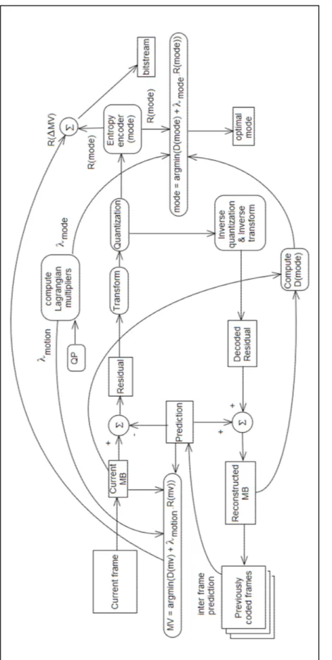
In a more detailed picture, the encoder in Figure 1.8 contains some of the elements of the RDO mechanism as well. The video source is represented by the current frame, from which the current MB is selected for encoding. The prediction model, which exploits both temporal and spatial redundancy, finds the best estimation (multiple prediction blocks when MB is partitioned as in Figure 1.3) from the previously encoded frames, and partially removes the redundancy between the original macroblock (MB) and the estimated one in spatial and temporal domains. This is where the RDO mechanism, by means of

λ

MOTION of the equation

(1.12), trades the number of bits to encode the MVs for the distortion calculated between the current and estimated MBs. Once the best prediction and MVs are found, the residual signal as a difference between the original MB and its prediction, motion compensated, is fed to the image model. The residual is transformed, quantized, inverse quantized and inverse transformed to produce the decoded residual which is added to the prediction to form the reconstructed MB. The optimal mode is concurrently decided via

λ

MODEof the equation

(1.13) that helps negotiate between the number of bits to encode the transformed and quantized coefficients, and the distortion D(mode), calculated between the reconstructed an the original MBs. The bits required to separately encode the MVs difference and the transformed/quantized coefficients of the best mode, are included into the final bitstream.

In the current reference implementation of H.264, the block that generates the Lagrangian multipliers for the ME and MD stages, uses empirical values and is totally independent of any of the processing blocks in the diagram. In this research, we improve the design by

24

Figure 1.8 H.264 encoder block diagram

.

Adapted from (

Richardson, 2010

connecting it to the transform block of the mode decision loop and propose a new algorithm to dynamically adapt the Lagrange multipliers with the image content, thereby improving the performance in terms of rate-distortion.

CHAPTER 2

LITERATURE OVERVIEW 2.1 Lagrange multiplier selection

In H.264/AVC standard the Lagrange multiplier selection occurs at both motion estimation and mode decision levels, this is why it has 2 components:

λ

MOTION and

λ

MODE. Yet, only

when the SSE metric is utilized in both processes these values are deemed equal, which is in line with the way the distortion (PSNR) is calculated. The value of

λ

MOTION displays a weak

dependency on the search precision (FPel, HPel, QPel) and method (full search, UMHexagon, EPZS with its refinement patterns) utilized in motion estimation. The best prediction of a macroblock, once established, is used throughout the mode decision process to establish the best trade-off between rate and distortion achievable for a certain encoding mode. Even with a suboptimal prediction (generated by a sub-optimal search method) the mode decision is the one that finally decides what is the best mode for a macroblock to be encoded with, so the mode decision outweighs in importance the motion estimation stage. It becomes stringent that the value of Lagrange multiplier is the right one, especially for the mode decision stage; and this is an area where the research has been focusing in the latest decade.

Currently, the reference software (Sühring, 2013) allows the encoding of the current MB by using up to 16 frames as reference. A frame is encoded using one of the patterns I, P, B. To encode a P frame, each MB, based on the RDO mode decision, (High, High Fast, and Low) can be encoded as 16x16 8x16 16x8, 8x8 and each block from an 8x8 partition can be encoded as an 8x4, 4x8 or 4x4 block. To encode a 4x4 block pertaining to I-type frame there are 9 possibilities based on the samples supplied by the neighborhood.

Besides, in the process of the motion estimation, there are multiple ways of finding the best match for a MB given the reference frame(s).

28

When the discrete J cost function is calculated for a MB all these possibilities come into play, and the optimum value is the one for which the minimum of J is achieved among the entire set of possible configurations.

The H.264/AVC reference software implements a one-step encoding algorithm at the macroblock level, where the value of Lagrange multiplier is calculated by taking into account the rate and distortion dependency on the quantization parameter QP only.

Even so, the experiments on multiple sequences, with slow and fast movement, along with the usage of different combinations of profiles and types (baseline, main, extended) have proven that the rate and distortion models (or similarity as a measure of visual conformance) also depend on many other factors among which the most important are the side information (macroblock header bits, MV bits, frame and macroblock type, entropy model), the source information, selection of the encoding modes, and especially the information contained in the transformed coefficients, as pointed out in (Li and others, 2009) and (Li and others, 2007).

Indeed, more accurate rate and distortion models would have to consider these parameters as well. The calculation of the Lagrange multiplier would then have to take into account the partial derivatives with respect to all these parameters, for both continuous and discrete cases. In this way, such models would get even closer to real data. Yet, an obvious downside would be the increasing computational effort that would occur in this case. This is why, in practice, the encoders follow the Wiegand-Girod RD model that depends on QP only (Wiegand and Girod, 2001).

A quadratic or exponential dependency with QP is expressed in the case of H.263 or H.264/AVC respectively. The rate-distortion model of Wiegand-Girod is based on the high rate assumption, which allows expressing the Lagrangian multiplier

λ

HR in terms of QP at

high rates. Any Lagrange multiplier expression, determined for any other model, should asymptotically converge to this value, as a measure of the new approach correctness. As such, the H.263 and even H.264/AVC adopted the

λ

HR approach, regardless of the motion

degree in the scene, which experimentally proved satisfactory in combination with the traditional distortion measures SAD, SATD, and SSE. Still, the high rate assumption might not hold true in the case of video conferences or slow-paced sequences (ex: container.yuv, bridge.yuv), where unnecessary bits might be sent into the resulting bitstream.

Since λHR is only related to QP, as long as the other dependencies mentioned beforehand are neglected,

λ

is not optimally calculated and the calculated values of the cost function J are higher, so the performance is weak.

The main drawback of the new models developed so far, resides in the fact that within the calculation of the Lagrangian multiplier, the derivatives of the rate and distortion are computed with respect to Q step (represented by the QP parameter) only.

Several trends related to bits allocation have been emerging in the recent years. Some of them try to fit the best probability distribution function with the residual signal distribution. Others replace the distortion with its complementary, which is based on a perceptual visual quality metric, to explore for the optimal expression of

λ

, or they combine the compression processes at the frame and macroblock levels successively optimizing for one parameter at a time.

Their performances, benefits, and drawbacks are featured in the following sections.

2.1.1 Laplace distribution-based approach for inter-frame coding

The articles (Li and others, 2009) and (Li and others, 2007) constitute the first step taken to model the rate and distortion functions from other perspective, beyond the traditional sole dependence of QP. The novelty of the proposed method consists in a new Lagrange multiplier determined at the frame level, equally applicable to all frame’s macroblocks, and adaptive with the frame’s statistics. The algorithm efficiency was proved especially in the case of the quasi-stationary sequences, though the authors needed to handle several special

30

cases where the theoretical assumptions and the proposed model did not fit with the real-world use.

There are several great contributions and interesting standpoints in this article, as follows: 1) The derived RD models are based on the zero-mean Laplace distribution of the coefficients resulting from the transformed residuals. The Laplace parameter Λ and the standard deviation σ of the transformed residuals are related as follows:

2 σ

Λ = (2.1)

The zero-mean Laplace distribution is defined as: ( | |) ( )

2

Lap x

f x = Λe −Λ (2.2)

The Laplace distribution was chosen among other distributions (Cauchy, Gauss) due to its single parameter Λ to be determined. It also has a good accuracy and a medium complexity of the calculation. The hypothesis of Laplace distribution of the transformed residuals overrides the high rate assumption, for it can be applied for low rate output too. Likewise, the standard deviation σ of the transformed residuals is strongly related to the source of video signal, being considered an inherent statistical property of the input sequence. Consequently, the Laplace distribution establishes itself as a unanimously agreed-upon choice for the representation of the input signal distribution.

2) The entropy H of the quantized transformed residuals is calculated based on the uniform reconstruction scalar quantizer, though, being dependent on the encoding method (CAVLC or CABAC), its expression roughly represents the rate model. The authors of (Li and others, 2009) refined the expression of the entropy, obtained on the following considerations:

- The probabilities of the transformed residuals, summed as the entropy, are calculated by integrating the Laplace pdf of the uniform quantized residuals, within the quantization intervals, corrected with the rounding offset

γ

. The offset constant values were separately determined for intra/inter encoding, though it could itself constitute another parameter for performance improvement.

- The classical form of the entropy (H= −



P.log2P) was corrected in order to handle the

case of skipped macroblocks and get as close as possible to the real rate.

- Since the entropy cannot further handle the final stages of the compression (run length and tree/arithmetic encoding), the authors were compelled to apply correction factors to the probability P0of quantized-zeroes (computed on the dead zone) and probability Pn of

quantized non-zeroes, respectively. The resulting rate model excludes the bitrate of the skipped macroblocks.

- The ratior P P= s/ 0, where Ps is the probability of the skipped blocks and P0 represents the percentage of the quantized zeroes per frame, is always sub unit. Therefore, this derived parameter is considered as an inherent property of the input sequence too.

- A roughly linear dependency relationship, at the practical QP = 28..40 values, was

experimentally noticed between ln( /R Hrefined)and the product (Λ.Q). The linearity constant S was determined under the convergence condition.

3) The closed form of the distortion model is determined by summing the second moment of the Laplace pdf on each quantization interval.

4) The authors proved that for uniform distribution, which can be obtained from Laplace distribution when

Λ →

0

:

2

( . )

Lap HR

cQ

λ

→

λ

=

(2.3)

as in the case of H.263. It means that when the Laplace signal extends to all frequencies spectrum (

σ

→∞), λLapbecomes a particular case ofλHR.

5) This is an adaptive algorithm whose parameters values (Λ , r) in the current frame are estimated from the ones collected in the previous (up to five) frames. With the predicted