Numerical study of a sinusoidal transverse propeller

(1)

Science Arts & Métiers (SAM)

is an open access repository that collects the work of Arts et Métiers Institute of Technology researchers and makes it freely available over the web where possible.

This is an author-deposited version published in: https://sam.ensam.eu Handle ID: .http://hdl.handle.net/10985/15002

To cite this version :

G. FASSE, Annie-Claude BAYEUL-LAINE, Olivier COUTIER-DELGOSHA, A. CURUTCHET, B. PAILLARD, F. HAUVILLE - Numerical study of a sinusoidal transverse propeller - IOP Conference Series: Earth and Environmental Science - Vol. 240, p.052007 - 2019

Any correspondence concerning this service should be sent to the repository Administrator : archiveouverte@ensam.eu

(2)

IOP Conference Series: Earth and Environmental Science

PAPER • OPEN ACCESS

Numerical study of a sinusoidal transverse propeller

To cite this article: G Fasse et al 2019 IOP Conf. Ser.: Earth Environ. Sci. 240 052007

(3)

Content from this work may be used under the terms of theCreative Commons Attribution 3.0 licence. Any further distribution of this work must maintain attribution to the author(s) and the title of the work, journal citation and DOI.

Published under licence by IOP Publishing Ltd

29th IAHR Symposium on Hydraulic Machinery and Systems

IOP Conf. Series: Earth and Environmental Science 240 (2019) 052007

IOP Publishing doi:10.1088/1755-1315/240/5/052007

1

Numerical study of a sinusoidal transverse propeller

G Fasse 1_{, A C Bayeul-Lainé}1*_{, O Coutier-Delgosha}1, 4_{, A Curutchet}2_{, B Paillard}2_, F Hauville3

1_{Univ. Lille, CNRS, ONERA, Centrale Lille,}1_{Arts et Metiers ParisTech, FRE 2017,}

Laboratoire de Mécanique des Fluides de Lille – Kampé de Fériet, F-5900, Lille, France

2_{ADV TECH SAS, 34 rue Richard WAGNER, 33700, Mérignac, France}

3_{Department of Mechanical Engineering, Naval Academy Research Institute, 29160,}

Lanvéoc, France

4_{Virginia Tech, Kevin T. Crofton Dept. of Aerospace & Ocean Engineering,}

Blacksburg 24060 VA, USA

*_{Annie-claude.bayeul-laine@ensam.eu}

Abstract. In order to obtain higher propulsion efficiency for marine transportation, the authors have numerically tested a novel trochoidal propeller using a sinusoidal blade pitch function. The main results presented here are the evaluation of thrust and torque, as well as the calculated hydrodynamic efficiency, for various absolute advance coefficients. The performance of the present sinusoidal-pitch trochoidal propeller is compared with previous analytical calculations of transverse propeller performances. Calculations for the trochoidal propeller are performed using a two-dimensional model. The numerical calculation is used to optimize the foil pitch function in order to achieve the highest efficiency for a given geometry and operational parameters. Foil-to-foil interactions are also studied for multiple-foil propellers to determine the effects of the blade number on the hydrodynamic efficiency.

1. Introduction

In the fuel-reduction and higher energy efficiency current context in marine transportation, investigations of alternative marine propeller are continuously expanding. Moreover, by bio-mimetic fish swimming can be very instructive to developing unconventional propeller as a result of many million years of evolutionary optimization. By oscillating their body or fins, marine animals use the energy dissipated in the wake vortices which are characteristic of thrust generation. The propulsion of

marine animals has been studied since the beginning of 20th_{century but more accurate studies have}

been undertaken at the end of 20th_{century (Anderson et al [1-2]). Li-Ming et al [10] give also an}

interesting review of underwater bio-mimetic propulsion.

The transverse axis propellers, which are combining two rotations (Voith-Schneider and Lipp rotor) or combining a translation and a beat (flapping foil thrusters) can model marine animal swimming [1-9, 10-16]. In this paper only the first ones were studied. The operation of a marine thruster with a transverse axis is very different from that of conventional axial propellers. It is characterized by the rotation of several blades around a vertical axis, associated with a motion of each blade around its own axis. The advantage of these systems is to generate a 360° vector thrust force. The blades’ kinematics produce a horizontal thrust whose hydrodynamic efficiency depends strongly on the law of control of the blades. Some concepts were proposed in the past for thrusters and

(4)

implemented for very specific applications. The Voith-Schneider propeller, for example, provides a fast-thrust response in any direction, which improves dramatically the manoeuvrability of ships that are equipped with it. However, its epicycloid kinematics imposes a peripheral speed larger than the speed of the ship, which restricts its use to service vessels (tug, ferry, buoyage ...) at low ship speed (up to 15knots). Conversely, thrusters with trochoidal kinematics whose peripheral speed is lower than the speed of the ship allow considering much higher speeds of advance. A major challenge of this approach is the study and the optimization of the shape and kinematics of the propulsion system blades. Modern CFD solvers, combined with the optimization methods to which they are now coupled, offer new perspectives in this regard. In this context, a numerical study, to analyse the flows in these machines with transverse axis, has been initiated to optimize the kinematics of the blades and therefore their efficiency. The results will be compared to those of Roesler [13].

2. Description of the propeller

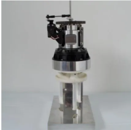
The reference propeller is the propeller designed by ADV TECH and shown in figure 1. The influence of the number of blades, of solidity and of calibration angle are analysed in this study. For the numerical study, table 1 gives the geometry setup.

Table 1. Calculations parameters.

Name Symbol Value

Rotor radius R 0.03 m

Number of blades n 3 or 4

Blade chord c 0.03 m

Position of blade’s

rotation center ¼ chord

Blade type NACA

0012

Figure 1. ADV TECH Trochoidal propeller. 3. Definition of parameters

Considering that the depth of the blades is much higher than the chord and by neglecting the effect of winglet, it is assumed that a 2D calculations will provide good comparisons and eventually the optimized parameters in order to obtain the best compromise between a good efficiency and the best trust properties. 3D calculations will be done later in order to check the influence of the third dimension.

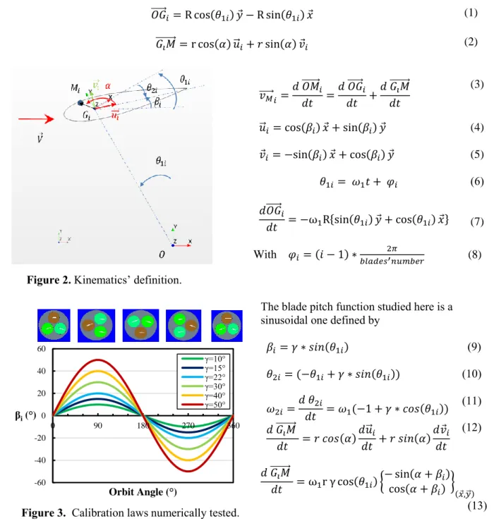
The kinematics of a blade i is presented here. In this propeller, two kinds of rotations have to be

considered: the first one around the major centre O (𝜃_1𝑖) and another one (𝜃2𝑖) which is more an

oscillation rather than a complete rotation around a centre of rotation of the foil, Gi, generally situated

at the ¼ of the chord near the leading edge (figure 2).

Equations (1) to (3) enable to derive the velocity of a point M on the blades depending on the two rotations. The local reference frame is defined by equations (4) and (5). Equation (6) defines the orbit

angle 𝜃1𝑖 of center’s blade i, Gi, between 𝑦⃗ axis and 𝑂𝐺⃗⃗⃗⃗⃗⃗⃗⃗⃗. Equation (7) gives the contribution of the _𝑖

first rotation in the determination of the velocity of the point M. The influence of the second movement is given by the kinematics and by equations (9) to (12). Equation (13) gives the contribution of the second rotation in the determination of the velocity of the point M.

The calibration law defines the angle of incidence i which is the sinusoidal expression given by equation (9). Different values of amplitude  were tested (10, 15, 22, 30, 40 and 50°) for the first

(5)

IOP Publishing doi:10.1088/1755-1315/240/5/052007 3 𝑂𝐺 ⃗⃗⃗⃗⃗⃗_𝑖_{= R cos(𝜃}_1𝑖) 𝑦⃗ − R sin(𝜃_1𝑖) 𝑥⃗ (1) 𝐺𝑖𝑀 ⃗⃗⃗⃗⃗⃗⃗⃗ = r cos(𝛼) 𝑢⃗⃗𝑖+ 𝑟 sin(𝛼) 𝑣⃗𝑖 (2) 𝑣𝑀 ⃗⃗⃗⃗⃗⃗_𝑖 =𝑑 𝑂𝑀⃗⃗⃗⃗⃗⃗⃗𝑖 𝑑𝑡 = 𝑑 𝑂𝐺⃗⃗⃗⃗⃗⃗𝑖 𝑑𝑡 + 𝑑 𝐺⃗⃗⃗⃗⃗⃗⃗⃗𝑖𝑀 𝑑𝑡 (3) 𝑢⃗⃗𝑖 = cos(𝛽𝑖) 𝑥⃗ + sin(𝛽𝑖) 𝑦⃗ (4) 𝑣⃗𝑖 = −sin(𝛽𝑖) 𝑥⃗ + cos(𝛽𝑖) 𝑦⃗ (5) 𝜃1𝑖 = 𝜔1𝑡 + 𝜑𝑖 (6) 𝑑𝑂𝐺⃗⃗⃗⃗⃗⃗𝑖 𝑑𝑡 = −ω1R{sin(𝜃1𝑖) 𝑦⃗ + cos(𝜃1𝑖) 𝑥⃗} (7) With 𝜑𝑖 = (𝑖 − 1) ∗ 2𝜋 𝑏𝑙𝑎𝑑𝑒𝑠′_{𝑛𝑢𝑚𝑏𝑒𝑟} (8)

Figure 2. Kinematics’ definition.

Figure 3. Calibration laws numerically tested.

The blade pitch function studied here is a sinusoidal one defined by

𝛽𝑖 = 𝛾 ∗ 𝑠𝑖𝑛(𝜃1𝑖) (9) 𝜃2𝑖 = (−𝜃1𝑖+ 𝛾 ∗ 𝑠𝑖𝑛(𝜃1𝑖)) (10) 𝜔2𝑖 = 𝑑 𝜃2𝑖 𝑑𝑡 = 𝜔1(−1 + 𝛾 ∗ 𝑐𝑜𝑠(𝜃1𝑖)) (11) 𝑑 𝐺⃗⃗⃗⃗⃗⃗⃗⃗ 𝑖𝑀 𝑑𝑡 = 𝑟 𝑐𝑜𝑠(𝛼) 𝑑𝑢⃗⃗𝑖 𝑑𝑡 + 𝑟 𝑠𝑖𝑛(𝛼) 𝑑𝑣⃗𝑖 𝑑𝑡 (12) 𝑑 𝐺⃗⃗⃗⃗⃗⃗⃗⃗ 𝑖𝑀 𝑑𝑡 = ω1r γ cos(𝜃1𝑖) { − sin(𝛼 + 𝛽𝑖) cos(𝛼 + 𝛽𝑖) }_{(𝑥⃗,𝑦⃗⃗)} (13) The common non-dimensional coefficients used for propellers are:

- Advance coefficient 

λ = 𝑉 𝜔⁄ 1. 𝑅 (14)

- Efficiency

𝜂 = 𝐹̅̅̅. 𝑉 𝑃𝑋 ⁄ 𝑢𝑠𝑒𝑓𝑢𝑙 (15)

where 𝐹̅̅̅ is the mean force generated by all blades during one cycle and 𝑃_𝑋 𝑢𝑠𝑒𝑓𝑢𝑙 is the power

required to drive the thruster, defined by the following equations for each blade:

-60 -40 -20 0 20 40 60 0 90 180 270 360 βi(°) Orbit Angle (°) γ=10° γ=15° γ=22° γ=30° γ=40° γ=50°

(6)

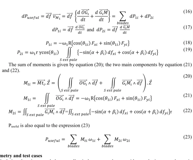
IOP Publishing doi:10.1088/1755-1315/240/5/052007 𝑑𝑃𝑢𝑠𝑒𝑓𝑢𝑙= 𝑑𝑓⃗⃗⃗⃗⃗ 𝑣⃗⃗⃗⃗⃗⃗⃗ = 𝑑𝑓_𝑀𝑖 ⃗⃗⃗⃗⃗ { 𝑑 𝑂𝐺⃗⃗⃗⃗⃗⃗⃗⃗𝑖 𝑑𝑡 + 𝑑 𝐺⃗⃗⃗⃗⃗⃗⃗⃗𝑖𝑀 𝑑𝑡 } = ∑ 𝑑𝑃1𝑖+ 𝑑𝑃2𝑖 𝑏𝑙𝑎𝑑𝑒𝑠 (16) 𝑑𝑃1𝑖 = 𝑑𝑓⃗⃗⃗⃗⃗ 𝑑 𝑂𝐺⃗⃗⃗⃗⃗⃗⃗⃗𝑖 𝑑𝑡 and 𝑑𝑃2𝑖 = 𝑑𝑓⃗⃗⃗⃗⃗ 𝑑 𝐺⃗⃗⃗⃗⃗⃗⃗⃗⃗𝑖𝑀 𝑑𝑡 (17) 𝑃1𝑖 = −ω1R{cos(𝜃1𝑖) 𝐹𝑥𝑖+ sin(𝜃1𝑖) 𝐹𝑦𝑖} (18)

𝑃2𝑖= ω1r γcos(𝜃1𝑖) ∬ {−sin(𝛼 + 𝛽𝑖) 𝑑𝑓𝑥𝑖+ cos(𝛼 + 𝛽𝑖) 𝑑𝑓𝑦𝑖}

𝑆 𝑒𝑥𝑡 𝑝𝑎𝑙𝑒

(19) The sum of moments is given by equation (20); the two main components by equation (21) and (22). 𝑀𝑡𝑖= 𝑀𝑡⃗⃗⃗⃗⃗⃗⃗⃗. 𝑍⃗ = (𝑖 ∬ 𝑂𝐺⃗⃗⃗⃗⃗⃗⃗⃗ ˄ 𝑑𝑓𝑖 ⃗⃗⃗⃗⃗ 𝑆 𝑒𝑥𝑡 𝑝𝑎𝑙𝑒 + ∬ 𝐺⃗⃗⃗⃗⃗⃗⃗⃗⃗⃗ ˄ 𝑑𝑓𝑖𝑀𝑖 ⃗⃗⃗⃗⃗ 𝑆 𝑒𝑥𝑡 𝑝𝑎𝑙𝑒 ) . 𝑍⃗ (20) 𝑀1𝑖 = ∬ 𝑂𝐺⃗⃗⃗⃗⃗⃗⃗⃗ ˄ 𝑑𝑓𝑖 ⃗⃗⃗⃗⃗ 𝑆 𝑒𝑥𝑡 𝑝𝑎𝑙𝑒 = −ω1R{cos(𝜃1𝑖) 𝐹𝑥𝑖+ sin(𝜃1𝑖) 𝐹𝑦𝑖} (21) 𝑀2𝑖 = ∬_{𝑆 𝑒𝑥𝑡 𝑝𝑎𝑙𝑒}𝐺⃗⃗⃗⃗⃗⃗⃗⃗⃗⃗ ˄ 𝑑𝑓𝑖𝑀𝑖 ⃗⃗⃗⃗⃗=∬_{𝑆 𝑒𝑥𝑡 𝑝𝑎𝑙𝑒}{−sin(𝛼 + 𝛽𝑖) 𝑑𝑓𝑥𝑖+ cos(𝛼 + 𝛽𝑖) 𝑑𝑓𝑦𝑖}r (22)

Puseful is also equal to the expression (23) 𝑃𝑢𝑠𝑒𝑓𝑢𝑙= ∑ 𝑀𝑡𝑖

𝑏𝑙𝑎𝑑𝑒𝑠

𝜔1𝑖+ ∑ 𝑀2𝑖

𝑏𝑙𝑎𝑑𝑒𝑠

𝜔2𝑖 (23)

4. Geometry and test cases

The calculation domain around the propeller is large enough to avoid perturbations, as shown in figure 4 (the drawing does not respect the scale). Boundary conditions are:

- Velocity inlet to simulate the vessel’s velocity of 1 m/s in the left boundary of the model

(Average Rec=3 104).

- Symmetry planes for lateral boundaries of the domain.

- Pressure outlet at the right boundary of the domain.

The model of the thruster, for n blades, contains (n+2) zones: Outside Domain of turbine, (n)

blades zones named Bladei Domain and zone between outside zone and blades zones named Turbine

Zone. Except outside zone, all other zones have relative motions. The mesh method used for these calculations is Sliding Mesh. Therefore, (n+1) interfaces between zones were created: an interface zone between outside and turbine zone and an interface between each blade and turbine zone. Details of the zones can be seen in figure 4 (the ratio scale is not respected for the drawing).

Table 2. Mesh parameters.

Domain Target size (%)

Outer domain 50

Wake 10

Blade’s zones 2

Figure 4. Definition of the different zones and

(7)

5

Calculations were done with Star CCM+ v11.06/12.06 URANS code. A polygonal mesh with prism layer around blades is used. The global mesh size is about 100,000 cells. All the dimensions of cells depend of the chord length (0.03m). These dimensions are given in table 2. Near the blades, 20

prism layers with a growth rate of 1.2 and a first cell size of 10−5_{m are defined to ensure the condition}

𝑦_{𝑤𝑎𝑙𝑙}+ < 1.

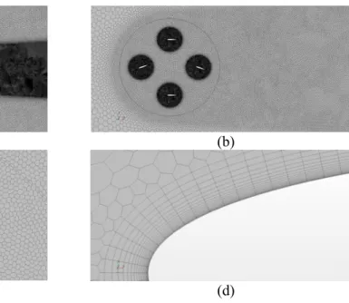
(a) (b)

(c) (d)

Figure 5. Mesh.

The mesh is presented in figure 5: (a) global mesh ;(b), focus on the turbine zone; (c), focus on blade’s zone; (d) focus on prism layer around a blade.

Two-dimensional incompressible Reynolds averaged Navier–Stokes equations are solved in unsteady states. The SST k- turbulence model is used. Calculations were realized for a propeller

advance velocity of 1 m/s. This leads to a value of Reynolds number of 3 104

.

For each calculation, the forces and moments are registered for each orbit angle (the time step is equal

to 𝑑𝜃1= 1°) after converged results (corresponding to 5 periods of principal rotation).

5. Results

5.1 First campaign of tests

Figure 6. Efficiency of the propeller as a function of

advance coefficient for different values of 

A first campaign of calculations has been done in case of n=3 and for a solidity of 𝜎 = 1,4.

Results of Efficiency 𝜂 defined by equation (15) are given in figure 6 in function of the advance parameter 𝜆. The results collected during this first campaign indicate that the highest efficiency is for 15° < 𝛾 < 22° and for 1,2 < 𝜆 < 2,3. When 𝛾 is higher than 30°, the efficiency is falling below 40% with values of 𝜆 lower than 1 (cycloidal motion), which is not interesting for the trochoidal propeller. 0 0,1 0,2 0,3 0,4 0,5 0,6 0,7 0 0,5 1 1,5 2 2,5 3 η λ γ=15° γ=22° γ=30° γ=40° γ=50°

(8)

So, as the best results of efficiency were obtained for 15° < 𝛾 < 22°, a second campaign of calculations was conducted to evaluate the best performance for a value of wedging angle around 20°. 5.2 Second campaign of tests

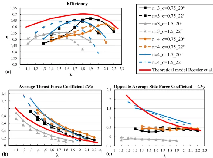
For this second campaign, two values of 𝛾 are tested: 20° and 22°. Influence of solidity is also considered by changing the blade number or the propeller radius (chord is always fixed at 0.03m). Global results are summarized in figure 7, concerning the efficiency, the average thrust force

coefficient CFx and the opposite average side force coefficient -CFy.

Figure 7. (a) Efficiency versus advance parameter, (b) Non-dimensional Average Thrust versus

advance parameter, (c) Non-dimensional Average Side Force versus advance parameter . The average thrust and side force coefficients are given by the following expressions:

𝐶𝐹𝑥 ̅̅̅̅̅ = 𝐹̅̅̅𝑋 0,5𝜌𝑐𝑉2 (25) and 𝐶̅̅̅̅̅ =𝐹𝑦 𝐹𝑌 ̅̅̅ 0,5𝜌𝑐𝑉2 (26)

Where 𝐹̅̅̅ is the average thrust given by all blades during one rotation and 𝐹_𝑋 ̅̅̅ is the average force 𝑌

in transverse direction given by all blades during one period of the principal rotation.

The present results are compared with theoretical model of Roesler et al. [13]. These authors studied a transverse propeller with the following parameters: 𝑛 = 4, 𝜎 = 1,89 , 𝑅 = 0,625 m, NACA

0,3 0,35 0,4 0,45 0,5 0,55 0,6 0,65 0,7 0,75 1 1,1 1,2 1,3 1,4 1,5 1,6 1,7 1,8 1,9 2 2,1 2,2 2,3 η λ Efficiency n=3_σ=0.75_20° n=3_σ=0.75_22° n=3_σ=1.5_20° n=3_σ=1.5_22° n=4_σ=0.75_20° n=4_σ=0.75_22° n=4_σ=1.5_20° n=4_σ=1.5_22°

Theoretical model Roesler et al.

(a) 0 0,2 0,4 0,6 0,8 1 1,2 1,4 1 1,1 1,2 1,3 1,4 1,5 1,6 1,7 1,8 1,9 2 2,1 2,2 2,3 λ

Average Thrust Force Coefficient 𝐶𝐹𝑥

(b) -0,5 0 0,5 1 1,5 2 2,5 1 1,1 1,2 1,3 1,4 1,5 1,6 1,7 1,8 1,9 2 2,1 2,2 2,3 λ

Opposite Average Side Force Coefficient - CFy

(9)

7

0015 (linearly tapered to a NACA 0008 at the tip), 𝑅𝑒_𝑐~105 and with a sinusoidal blade control law

with 𝛾 = 20°. The theoretical model is based on 2D potential code which includes 3D and viscous effects corrections (Roesler et al. [12-13]).

Even if the dimensions are not the same, this study presents a good agreement with the theoretical model of Roesler. For efficiency, the little discrepancy is probably due to the difference between potential and URANS codes. The resolution of Reynolds Average Navier-Stokes equations leads to a better characterization of viscous effect (development and stalling vortices on blade surface), compared with a potential code (even if a correction is added in the theoretical model of Roesler) and takes into account the influence of the wake of each blade on the next one.

This second campaign shows that solidity has a huge impact on the efficiency and on the generated thrust. For a 3-blades configuration, a compact propeller leads to a lower efficiency and a lower thrust than a spaced propeller. For a 4-blades configuration, the behaviour is opposite, but smaller. The modification of calibration law 𝛾 leads to an offset of the efficiency peak. Lastly, this study also shows that the 3-blades and high solidity configuration leads to a positive side force generation unlike other configurations and Roesler theoretical model.

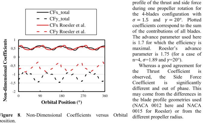
The figure 8 illustrates the profile of the thrust and side force during one propeller rotation for the 4-blades configuration with 𝜎 = 1.5 and 𝛾 = 20°. Plotted coefficients correspond to the sum of the contributions of all blades. The advance parameter used here is 1.7 for which the efficiency is

maximal. Roesler’s advance

parameter is 1.75 (for a case of n=4, 𝜎=1.89 and 𝛾=20°).

Whereas a good agreement for

the Thrust Coefficient is

observed, the Side Force

Coefficient is significantly

different and out of phase. This may come from the differences in the blade profile geometries used (NACA 0012 here and NACA 0015 for Roesler) or from the different propeller radius.

Figure 8. Non-Dimensional Coefficients versus Orbital

position.

Figure 9 shows the wake vortices by the visualisation of the z-vorticity. Red vortices represent counter clockwise circulation, and blue vortices represent clockwise circulation. It can be seen in this figure that for the 3-blades configuration, the highest efficiency is obtained when vortices in the wake are less intense than for a bad efficiency. The energy lost during vortices formation is not used for the propulsion effect. The flow is also more perturbed when the vortices are more intense. For the 4-blades configuration, no similar conclusion can be drawn.

-2 -1,5 -1 -0,5 0 0,5 1 0 90 180 270 360 N on -dim ensi onal C oef fi ci ents Orbital Position (°) CFx_total CFy_total CFx Roesler et al. CFy Roesler et al.

(10)

1i=0° 1i=30° 1i=60° 1i=90°

(a) n=3, =0.75, =20°, =1.9 =>  = 0.66 BEST EFFICIENCY

(b) n=3, =0.75, =20°, =1.3 =>  = 0.46

(c) n=3, =1.5, =20°, =1.5 =>  = 0.557 BEST EFFICIENCY

(d) n=3, =1.5, =20°, =1.1=>  =0.468

(e) n=4, =1.5, =20°, =1.6 =>  = 0.64

(f) n=4, =1.5, =20°, =1.3 =>  =0.59 Figure 9. Z Vorticity for 2 and 4 blades. 6. Conclusions

This paper has presented some numerical results, which characterize the performance of a trochoidal propeller employing a sinusoidal blade pitch function. The influence of some parameters has been studied:

- the influence of solidity

- the influence of number of blades

- the influence of wedging angles

- the influence of absolute advance coefficient

The global and the local results can be used in the future to optimize the foil pitch function in order to achieve the highest efficiency in marine propulsion system design.

(11)

9

- The influence of the Reynolds effect on global results (forces, power, efficiency…)

- The analysis of pressure distribution on the blades in order to detect cavitation apparition

zones.

- The examination of the evolution of loads and torques on each blade depending of the

azimuthal angle of the blade in order to study when the blade is propulsive or resistant and to detect the influence of the forward blade onto the backward blade.

- The influence of blade profile such as NACA 0015 and NACA 0018 or asymmetric shape in

order to optimize efficiency and thrust generation.

Nomenclature

c Blade’s chord (m) 𝑟 Radial coordinate of a point Mi of the

blade in cylindrical local coordinate

system (Gi, 𝑢⃗⃗⃗⃗, 𝑣_𝑖 ⃗⃗⃗⃗) _𝑖

𝐹𝑋

̅̅̅ Mean force given by all blades during one

cycle in the vessel advance direction (N)

R Radial position of the blade’s centre

(R=OGi)

𝐹𝑌

̅̅̅ Mean force given by all blades during one

cycle in the transverse direction (N)

V Propeller advance velocity in the direction

𝑋⃗

Fxi Instantaneous force in x direction for

azimuthal angle 𝜃1𝑖 and blade i

𝛼 Tangential coordinate of point Mi angle

Fyi Instantaneous force in y direction for

azimuthal angle 𝜃1𝑖 and blade i

𝛽𝑖 Angle between blade’s chord and 𝑋 ⃗⃗⃗⃗ axis

Gi Centre of blade flapping 𝛾 Maximal value of 𝛽_𝑖 : wedging angle

Mi Point on blade i  Absolute advance coefficient = 𝑉/𝜔₁𝑅

Mti Total moment (mN)on blade i/O 𝜑𝑖 Angle of phase shift of blade i

M1i Moment of local forces on blade i/Gi 𝜃_1𝑖 Azimutal’s angle of centre’s blade i, Gi

(between 𝑦⃗ axis and 𝑂𝐺⃗⃗⃗⃗⃗⃗⃗⃗⃗) 𝑖

M2i Moment of forces (Fxi and Fyi)on Gi/O

(mN)

𝜃2𝑖 Local rotation’s angle of blade i in

reference frame (𝑢⃗⃗⃗⃗, 𝑣𝑖 ⃗⃗⃗⃗) 𝑖

Puseful Useful power (W)  Solidity=𝑛𝑐/2𝑅

P1 First part of useful power (W) 𝜌 Density of fluid (water 998 𝑘𝑔. 𝑚−3)

P2 Second part of useful power (W) 1 Angular velocity of the propeller (rad.s-1)

n Number of blades (3 or 4) 𝜔2𝑖 Angular velocity of blade i (rad.s-1) in

reference frame (𝐺𝑖, 𝑢⃗⃗⃗⃗, 𝑣𝑖 ⃗⃗⃗⃗) 𝑖

References

[1] Anderson J 1996 Vorticity control for efficient propulsion PhD thesis, Massachusetts Institute of

Technology and Woods Hole Oceanographic, Institution, Cambridge, MA.

[2] Anderson J, Streitlien K, Barrett D and Triantafyllou M 1998 Oscillating foils of high

propulsive efficiency J Fluid Mech 360 41–72.

[3] Ashraf M A , Young J. and Lai, J C S 2011 Numerical Analysis of an Oscillating-Wing Wind

and Hydropower Generator, AIAA Journal, Vol. 49 No. 7

[4] Azuma A and Watanabe T 1988 Flight performance of a dragonfly J Exp Biol 137 1 221–252

[5] Bucur D M, Dunca G, Georgescu S C, Georgescu A M 2016 Water flow around a flapping foil:

preliminary study on the numerical sensitivity U.P.B. Sci. Bull. Series D Vol. 78

[6] Epps B P, Muscutt L E, Roesler B T, Weymouth G D and Ganapathisubramani B 2016 On the

Interfoil Spacing and Phase Lag of Tandem Flapping Foil Propulsors J Ship Prod Des Vol. 32

No. 4 1–7

(12)

fish-like motion pattern Computers and Fluids 156 305–316

[8] Kinsey T,Dumas G 2006 Parametric Study of an Oscillating Airfoil in Power Extraction Regime, AIAA

Journal

[9] Li-Ming C, Yong-Hui C, Guang P 2017 A review of underwater bio-mimetic propulsion: cruise

and fast-start Fluid Dyn. Res. Vol. 49 No 4

[10] Posri A, Phoemsapthawee S, Nonthipat T 2018 Viscous investigation of a flapping foil propulsor IOP Conf. Ser.: Mater. Sci. Eng. 297

[11] Osama M 2001 Experimental Investigation of Low Speed Flow Over Flapping Airfoils and Airfoil Combinations PhD Thesis

[12] Roesler T, Francisquez M, Epps B 2014 Design and Analysis of Trochoidal Propulsors using Nonlinear Programming Optimization Techniques, Proc. of the ASME,33 rd Int. Conf. on Ocean, San Francisco

[13] Roesler B T, Kawamura M L, Miller E, Wilson M, Brink-Roby J, Clemmenson E, Keller M, Epps, B P 2016 Experimental Performance of a Novel Trochoidal Propeller. J. Ship Research.

60 48-60

[14] Sanchez-Caja A and Martio J 2016 On the optimum performance of oscillating foil propulsors J

Mar Sci Technol

[15] Young J, Ashraf M A, Lai J C S,Platzer M F 2013 Numerical simulation of fully passive flapping foil power generation AIAA Journal vol. 51 2727-39

[16] Young J, Lai J C S, Platzer M F 2014 A review of progress and challenges in flapping foil power generation Progress in Aerospace Sciences 67 2–28

[17] Young J, Lai J C S, Platzer M F 2015 Flapping Foil Power Generation: Review and Potential

in Pico-Hydro Application Int. Conf. on Sustainable Energy Engineering and Application