POLYTECHNIQUE MONTRÉAL
affiliée à l’Université de Montréal
Deep Learning and Reinforcement Learning for Inventory Control
ZAHRA KHANIDAHAJ
Département de mathématiques et de génie industriel
Mémoire présenté en vue de l’obtention du diplôme de Maîtrise ès sciences appliquées Génie industriel Décembre 2018 © ZahraKhanidahaj, 2018.
POLYTECHNIQUE MONTRÉAL
affiliée à l’Université de Montréal Ce mémoire intitulé :
Deep Learning and Reinforcement Learning for Inventory Control
présenté par Zahra KHANIDAHAJ
en vue de l’obtention du diplôme de Maîtrise ès sciences appliquées
a été dûment accepté par le jury d’examen constitué de :
Michel GENDREAU, président
Louis-Martin ROUSSEAU, membre et directeur de recherche
DEDICATION
ACKNOWLEDGEMENTS
First of all, I would like to thank my supervisor, Professor Louis-Martin Rousseau, for his valuable guidance and continuous technical and financial supports during my research. In addition, I express my sincere gratitude to Dr. Yossiri Adulyasak, for his technical support during my project.
Also, I would like to express my appreciation to my thesis committee members, Professor Michel Gendreau and Professor Andrea Lodi for their time and constructive comments. In Addition, I appreciate my intimate friends for their helps during this period.
Many thanks go to Dr. Joelle Pineau and Dr. Doina Precup at McGill University. I augmented my knowledge about deep learning and reinforcement learning considerably by the valuable comments and discussions during their courses.
And last but not least, special thanks to my beloved family. I cannot find any word expressing my deepest thanks and appreciation. I am highly in my dear family’s debt for their endless support and unconditional love and encouragement even I am thousands of kilometres far from home. They have always been helping me to pursing my goals and been supporting me continuously, throughout my life.
RÉSUMÉ
La gestion d’inventaire est l’un des problèmes les plus importants dans la fabrication de produits. Les décisions de commande sont prises par des agents qui observent les demandes, stochastiques, ainsi que les informations locales tels que le niveau d’inventaire afin de prendre des décisions sur les prochaines valeurs de commande. Étant donné que l’inventaire sur place (la quantité disponible de stock en inventaire), les demandes non satisfaites (commandes en attente), et l’existence de commander sont coûteux, le problème d’optimisation est conçu afin de minimiser les coûts. Par conséquent, la fonction objective est de réduire le coût à long terme) dont les composantes sont des inventaires en stock, commandes en attente linéaires (pénalité), et des coûts de commandes fixes.
Généralement, des algorithmes de processus de décision markovien, et de la programmation dynamique, ont été utilisés afin de résoudre le problème de contrôle d’inventaire. Ces algorithmes ont quelques désavantages. Ils sont conçus pour un environnement avec des informations disponibles, telles que la capacité de stockage ou elles imposent des limitations sur le nombre d’états. Résultat, les algorithmes du processus de décision markovien, et de la programmation dynamique sont inadéquats pour les situations mentionnées ci hauts, à cause de de la croissance exponentielle de l’espace d’état. En plus, les plus fameuses politique de getsion d’inventaire, telles que politiques standards <s,S> et <R,Q> ne fonctionne que dans les systèmes où les demandes d’entrées obtiennent une distribution statistique connues.
Afin de résoudre le problème, un apprentissage par renforcement approximée est développé dans le but d’éviter les défaillances mentionnées ci hauts. Ce projet applique une technique d’apprentissage de machine nommé ‘Deep Q-learning’, qui est capable d’apprendre des politiques de contrôle en utilisant directement le ‘end-to-end RL’, malgré le nombre énorme d’états. Aussi, le modèle est un ‘Deep Neural Network’ (DNN), formé avec une variante de ‘Q-learning’, dont l’entrée et la sortie sont l’information locale d’inventaire et la fonction de valeur utilisée pour estimer les récompenses futures, respectivement.
Le Deep Q-learning, qui s’appelle ‘Deep Q-Network’ (DQN), est l’une des techniques pionnières ‘DRL’ qui inclut une approche à base de simulation dans laquelle les approximations d’actions sont menées en utilisant un réseau DNN. Le système prend des décisions sur les valeurs de
commande. Étant donnée que la fonction de coût est calculée selon l’ordre ‘O’ et le niveau d’inventaire ‘IL’, les valeurs desquelles sont affectées par la demande ‘D’, la demande d’entrée ainsi que l’ordre et le niveau d’inventaire peuvent être considérés en tant qu’information individuelle d’inventaire. De plus, il y a un délai de mise en œuvre exprimant la latence dans l’envoi des informations et dans la réception des commandes. Le délai de mise en œuvre fournit davantage d’information locale incluant ‘IT’ et ‘OO’. Le ‘IT’ et ‘OO’ sont calculés et suivis durant les périodes de temps différents afin d’explorer plus d’informations sur l’environnement de l’agent d’inventaire. Par ailleurs, la principale information individuelle et la demande correspondante comprennent les états d’agents.
Les systèmes ‘PO’ sont davantage observés dans les modèles à étapes multiples dont les agents peuvent ne pas être au courant de l’information individuelle des autres agents. Dans le but de créer une approche basée sur le ‘ML’ et fournir quelques aperçus dans la manière de résoudre le type d’agent multiple ‘PO’ du problème actuel de contrôle d’inventaire, un agent simple est étudié. Cet un agent examine si on peut mettre sur pied une technique ‘ML’ basée sur le ‘DL’ afin d’aider à trouver une décision de valeur de commande quasi optimale basée sur la demande et information individuelle sur une période à long terme. Afin de le réaliser, dans un premier temps, la différence entre la valeur de commande (action) et la demande comme résultat d’un ‘DNN’ est estimée. Ensuite, la commande est mise à jour basée sur la commande à jour et la demande suivante. Enfin, le coût total (récompense cumulative) dans chaque étape de temps est mis à jour. En conséquence, résoudre le problème de valeur de commande d’agent simple suffit pour diminuer le coût total sur le long terme. Le modèle développé est validé à l’aide de différents ratios des coefficients de coût. Aussi, le rendement de la présente méthode est considéré satisfaisant en comparaison avec le ‘RRL’ (RL de régression), la politique <R,Q> et le politique
<s,S>. Le RL de régression n’est pas capable d’apprendre aussi bien et avec autant de précision
que le ‘DQN’. En dernier lieu, des recherches supplémentaires peuvent être menées afin d’observer les réseaux de chaînes d’approvisionnement multi-agents en série partiellement observables.
ABSTRACT
Inventory control is one of the most significant problems in product manufacturing. A decision maker (agent) observes the random stochastic demands and local information of inventory such as inventory levels as its inputs to make decisions about the next ordering values as its actions. Since inventory on-hand (the available amount of stock in inventory), unmet demands (backorders), and the existence of ordering are costly, the optimization problem is designed to minimize the cost. As a result, the objective function is to reduce the long-run cost (cumulative reward) whose components are linear holding, linear backorder (penalty), and fixed ordering costs.
Generally, Markov Decision Process (MDP) and Dynamic Programming (DP) algorithms have been utilized to solve the inventory control problem. These algorithms have some drawbacks. They are designed for the environment with available local information such as holding capacity or they impose limitations on the number of the states while these information and limitations are not available in some cases such as Partially Observable (PO) environments. As a result, DP or
MDP algorithms are not suitable for the above-mentioned conditions due to the enormity of the
state spaces. In addition, the most famous inventory management policies such as normal <s,S> and <R,Q> policies are desirable only for the systems whose input demands obtain normal distribution.
To solve the problem, an approximate Reinforcement Learning (RL) is developed so as to avoid having the afore-mentioned shortcomings. This project applies a Machine Leaning (ML) technique termed Deep Q-learning, which is able to learn control policies directly using end-to-end RL, even though the number of states is enormous. Also, the model is a Deep Neural Network (DNN), trained with a variant of Q-learning, whose input and output are the local information of inventory and the value function utilized to estimate future rewards, respectively. Deep Q-learning, which is also called Deep Q-Network (DQN), is one of the types of the pioneer Deep Reinforcement Learning (DRL) techniques that includes a simulation-based approach in which the action approximations are carried out using a Deep Neural Network (DNN). To end this, the agents observe the random stochastic demands and make decisions about the ordering values. Since the cost function is calculated in terms of Order (O) and Inventory Level (IL) whose values are affected by Demand (D), input demand as well as the order and inventory level can be
considered as the individual information of the inventory. Also, there is a lead-time expressing the latency on sending information or receiving orders. The lead-time provides more local information including Inventory Transit (IT) and On-Order (OO). IT and OO are calculated and tracked during different time periods so as to explore more information about the environment of the inventory agent. Furthermore, the main individual information and the corresponding demand comprise the states of the agent.
PO systems are observed more in multi-stage models whose agents can be unaware of the
individual information of the other agents. In order to create a ML-based approach and provide some insight into how to resolve the PO multi-agent type of the present inventory control problem, a single-agent is studied. This agent examines if one can implement a ML technique based on Deep Learning (DL) to assist to learn near-optimal ordering value decision based on demand and individual information over long-run time. To achieve this, first, the difference between the ordering value (action) and demand as the output of a DNN is approximated. Then, the order is updated after observing the next demand. Next, the main individual information of the agent called input features of a DNN is updated based on the updated order and the following demand. Lastly, the total cost (cumulative reward) in each time step is updated. Accordingly, solving the ordering value problem of single-agent suffices to diminish the total cost over long-run time. The developed model is validated using different ratios of the cost coefficients. Also, the performance of the present method is found to be satisfactory in comparison with Regression Reinforcement Learning (Regression RL), <R,Q> policy, and <s,S> policy. The regression RL is not able to learn as well and accurately as DQN. Finally, further research can be directed to solve the partial-observable multi-agent supply chain networks.
TABLE OF CONTENTS DEDICATION ... iii ACKNOWLEDGEMENTS ... iv RÉSUMÉ ... v ABSTRACT ... vii TABLE OF CONTENTS ... ix
LIST OF TABLES ... xii
LIST OF FIGURES ... xiii
LIST OF SYMBOLS AND ABBREVIATIONS ... xiv
CHAPTER 1 INTRODUCTION ... 1
1.1 Motivation and Objective ... 1
1.2 Problem Statement ... 3
1.2.1 Type of Inventory Model ... 5
1.2.2 DL and RL Components of DRL ... 6
1.3 Contributions ... 8
1.4 Thesis Structure ... 8 CHAPTER 2 A REVIEW OF INVENTORY CONTROL ... 9 CHAPTER 3 THEORY AND FORMULATION ... 13
3.1 Reinforcement Learning ... 13
3.3 Comparison of Different Techniques ... 14 3.3.1 Reinforcement Learning versus Supervised Learning ... 14
3.3.2 Reinforcement Learning versus Dynamic Programming ... 15
3.3.3 Q learning versus DQN ... 16 3.4 Different Types of Reinforcement Learning Algorithms ... 17 3.4.1 Q-learning ... 18 3.4.2 From RL to DQN ... 19 3.4.3 DQN ... 21 3.4.4 Optimizers ... 22 3.5 Exploration versus Exploitation (ϵ-greedy algorithms) ...
25 3.6 Improvement of DQN ...
25 CHAPTER 4 INVENTORY CONTROL SOLUTION ...
28 4.1 Main Features of Inventory Control ...
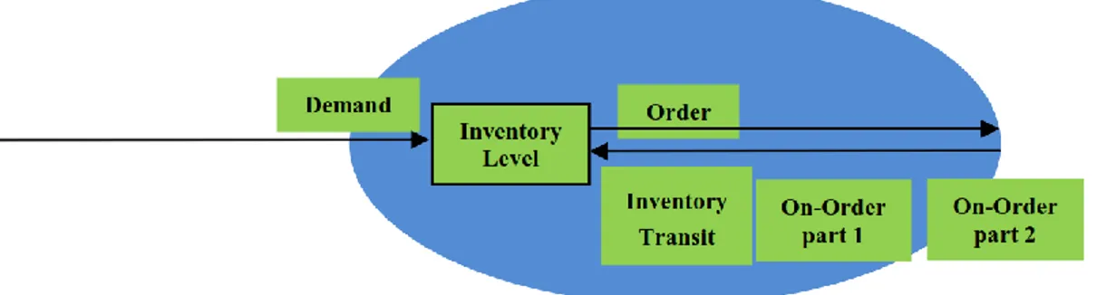
28 4.1.1 Random Features ...
28 4.1.2 Interrelated Features ...
28 4.2 Relations among Features ... 30
4.2.1 Relations among On-Order, Inventory Transition, and Order ... 30
4.2.2 Relations between Demand and Order ... 30
4.3 State Variables ... 31 4.4 Steps of Algorithm ... 32
4.4.1 Implementation of Frame Skipping and ϵ-greedy ... 32
4.4.2 DNN Section of Algorithm ... 33
4.4.3 Implementation of Experience Replay ... 35
4.4.4 Proposed DQN Algorithm ... 36 4.5 Hyperparameters Tuning ... 36
4.5.1 Reward, Inputs/Outputs and Hidden Layers of DQN ... 38
4.5.2 Frame and Batch Size ... 39
4.5.3 Activation Function and Type of Different Layers ... 39
4.5.4 Loss Function and Optimizer ... 40
4.5.5 Size of ER Memory, Updating Frequency, Learning Rate and ϵ ... 41 4.5.6 Running Environment and Setting Parameters ...
41 4.6 Experiments and Discussions ... 41
CHAPTER 5 SUMMARY, CONCLUSION, FUTURE WORKS, AND
RECOMMANDATIONS ... 49 BIBLIOGRAPHY ... 51
LIST OF TABLES
Table 1.1 Types of inventory model ... 5
Table 1.2 Components of inventory optimization problem for agent i, time t ... 6
Table 1.3 Different sections of DRL and its RL and DL sections ... 7
Table 4.1 Random features ... 29
Table 4.2 Interrelated features ... 29
Table 4.3 Main hyperparameters values ... 38 Table 4.4 The influence of replay and separation of the target Q-network ...
44 Table 4.5 Comparison between with/without of skipping frame ...
45 Table 4.6 Comparison of average cost for different coefficients and policies ...
LIST OF FIGURES
Figure 1.1 Input and output on single-stage inventory problem ... 4
Figure 1.2 The general mechanism for the sequence of events ... 5
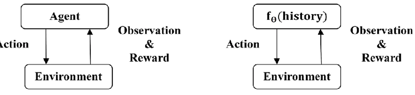
Figure 3.1 Interaction of agent with environment ... 13
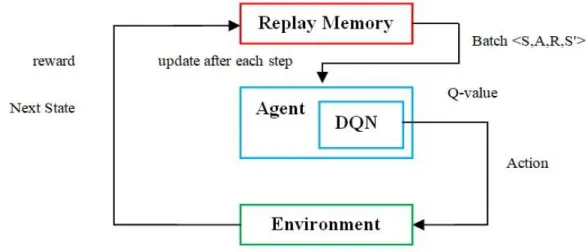
Figure 3.2 Q-learning (Left) versus DQN (Right) ... 17
Figure 3.3 Experience Replay (ER) in DQN ... 26
Figure 4.1 A general list of different parameters of an inventory agent ... 29
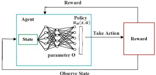
Figure 4.2 A general structure of DQN ... 32
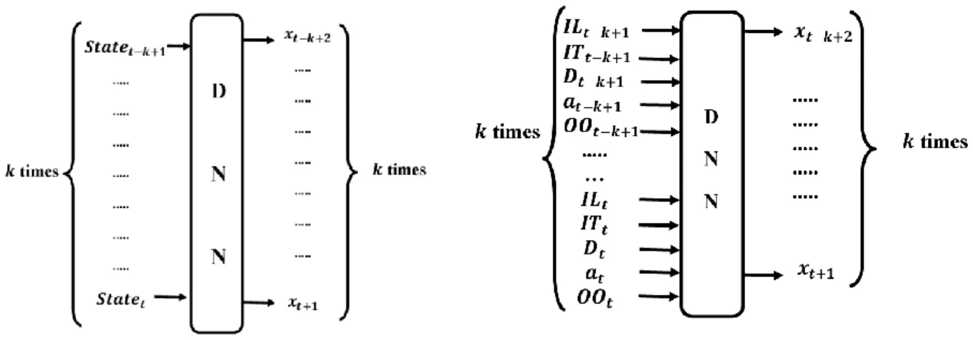
Figure 4.3 Function approximation based on feature extraction ... 34 Figure 4.4 The general I/O of DL approach for one agent used to estimate of difference between order and demand based on features of 𝑘 current states ... 34 Figure 4.5 The general structure of ϵ-greedy with DNN to update the state of one agent ... 34
Figure 4.6 The general implementation of ER with one agent in each time step ... 36
Figure 4.7 Comparison of different regression metrics and different optimizers ... 43
Figure 4.8 Comparison of different amount of learning rate and experience replay…... 43
Figure 4.9 Overall cost of different methods ... 45
Figure 4.10 Step-cost, IL, and O of different methods ... 46
LIST OF SYMBOLS AND ABBREVIATIONS
ADAM ADAptive Moment estimation
AI Artificial Intelligence
BP Back Propagation
DL Deep Learning
DNN Deep Neural Network
DQN Deep Q-Network
DRL ER
Deep Reinforcement Learning Experience Replay
FC Fully Connected
IID Independent and Identically Distributed
MAE Mean Absolute Error
MDP Markov Decision Process
ML Machine Learning
MSE Mean Square Error
NN Neural Network
POMDP Partial Observable Markov Decision Process PReLU Parametric Rectified Linear Unit
ReLU Rectified Linear Unit
RL Reinforcement Learning
SARSA State-Action-Reward-State-Action SGD Stochastic Gradient Descent
CHAPTER 1
INTRODUCTION
1.1 Motivation and ObjectiveInventory control is a well-known problem in the field of product manufacturing. Inventory controller (agent) decides about the ordering value based on the input demand in order to reduce the long-run total system cost consisting of linear holding, backorder, and fixed ordering costs. The unpredictability nature of the demand, which is due to its dynamic and random property, makes it reasonable to obtain a new approach to solve the inventory control problem even though there is a number of inventory models. Therefore, information-based decision making (using agents) is desirable. The current agent-based solutions induce some limitations on the values of data, which is not favorable generally. Accordingly, in the present research, a type of Deep Reinforcement Learning (DRL) method called Deep Q-Networks (DQN) is utilized to solve the inventory control problem.
A question can be raised why DRL is preferred to the other methods such as Dynamic Programming (DP), Reinforcement Learning (RL), and Deep Learning (DL). To answer this question, a detailed discussion based on the previous research works by Lin (1993), Van Roy et al. (1998), Mnih et al. (2013), Mnih et al. (2015), Van der Pol and Oliehoek (2017), and Sutton and Barto (2018) is presented in this section. In addition, a number of RL approaches for inventory control are described in Chapter 2. DP is inapplicable in most real problems because it is computationally very expensive. Also, most of the RL methods impose some limitations or require some pre-knowledge, which are not generally applicable. As a result, one of the long-term challenges of RL is to be able to learn how to control the agents directly from enormous inputs, similar to speech recognition. Most of the prosperous RL applications utilize hand-made features together with linear value functions or policy representation. Therefore, their performance is highly dependent on how good the features are. The advancement in DL makes the extraction of high-level features from raw datasets possible in some fields such as speech recognition. These approaches employed a type of DNN and both Supervised Learning (SL) and unsupervised learning. A comparative study of capabilities and incapabilities of RL, DL, and SL is presented herein. A RL method faces some challenges from a DL approach standpoint. For instance, DL techniques are applicable if a large value of labelled training data are available. However, RL
approaches should be able to learn from a frequently sparse, noisy, and delayed scalar reward. A large delay in observing the effect of an action on the reward is a negative point especially in comparison with the direct input-output relation in SL. Another challenge is that most DL approaches consider the independent data samplings, whereas RL techniques face sequences of much correlated states. In addition, the data distribution in a number of RL methods changes with the new behaviors learnt by the algorithm, whereas this can be a challenge for DL methods in which the data distribution is considered to be constant. The present research shows that a DNN can tackle the aforementioned problems so as to learn appropriate policies from raw datasets in complicated RL systems. To end this, a variant of the Q-learning method (Watkins and Dayan 1992) are utilized to train DNN using an optimizer for weight updates. The data correlation and non-stationary input distribution issues are mitigated by using Experience Replay (ER) sampling from the previous transitions at random, which makes the training distribution more accurate and smoother.
A Markov decision process (MDP) is a discrete time stochastic control process made of states, actions, rewards, and transition probabilities. Despite the fact that the problem with single product, single-stage, and a limited number of states (limitations on individual parameters and inputs) can be solved using MDP, the present research work is aimed at exploring a type of DRL approaches called DQN, obtaining some insights and examining the possibility of proper learning of the ordering value when there is no pre-knowledge or limitation on local information such as inventory capacity. This means that to reduce the long-run overall system cost, the stochastic random demands are the inputs, which affect the RL algorithm (a variant of Q-learning) whose actions are the ordering values approximated with the assistance of a DL. The inputs of this DNN structure are the important parameters (features) of inventory control including inventory level, inventory transit (inventory received in transit), on-order inventory (inventory sent but not received yet), ordering, and stochastic demand of the current time. Also, the output of DNN is the difference between the next order and the next demand (i.e. X=O-D). Since the stochastic demand of the next time is available as the input (D), the greedy calculation of the ordering value is conducted to be used by the ϵ-greedy rule. In addition, another input is lead-time (LT) which is equal to two. Consequently, the next time values of the other features and parameters such as inventory level (IL), inventory transit (IT), and on-order (OO) are calculated by the formulae presenting the relations between the different parameters on different
time steps (They are explained in more details in Chapter 4). Therefore, the updated versions of
IL, IT, OO, O, and D are the next inputs while approximation of the difference between the next
order and next demand (X=O-D) is the output of the next time of DNN (see Tables 1.2 and 1.3). The algorithm can be utilized without any limitation on some parameters such as inventory level, linear holding cost, linear backorder cost, different lead-time values, and type of demand distribution if it is determined.
1.2 Problem Statement
It is essential to gain the sufficient knowledge related to inventory control cost so as to respond to the inventory challenges. Tracking the inventory level (even positive or negative) and the number of times of ordering are unavoidable aspects of a successful inventory management in order to minimize the long-run total system cost. The components of this cost are linear holding, linear backorder (penalty), and fixed ordering costs associated with positive inventory level, negative inventory level, and the times of orders, respectively. The ordering value should be set to a near-optimal value so that the large number of times of ordering and the large values of holdings and backorders are avoided. In product manufacturing, the process of tracking incoming and outgoing goods (orders and demands) is called inventory management. The inventory management is investigated by an agent which makes decision about new orders (actions). This process is conducted after observing the stochastic input demands and by considering the inventory parameters in order to reduce the total cost (the long-run system cost).
Since there are some relations between components of individual information of the agent such as inventory transit, on-order value, and inventory level and the corresponding demand and order, in each time step, their next value is determined, the cumulative reward is updated, and the process continues until the last running time step. It should be mentioned that since the present solution is based on RL, “reward” is used instead of “cost” and their concepts are the same in this research.
Demand is observed as the input of inventory agent, while inventory controller makes decision about the order which is sent to the environment as its output (Figure 1.1). This decision is made by considering not only demand and order but also individual information of inventory such as inventory level. To capture the near-optimal overall cost of inventory, appropriate orders should be found as the outputs of inventory management.
Figure 1.1 Input and output on single-stage inventory problem
In order to solve this inventory control problem, an approach based on a combination of DL and RL is implemented so as to reduce the cumulative cost of an inventory agent which is executed on a long-run time. This aim is realized using a RL algorithm in which the difference between the action (order) and input (demand) is learned by a DNN. If the demand and order of each time step are considered as the parts of the individual information (state) of the decision maker (agent), the state of RL algorithm is the input of the DL section. The validation of the proposed technique is examined by comparing some methods such as <s,S> policy, <R,Q> policy and the regression RL approach.
In addition, each agent refers to one-stage decision maker in the inventory control optimization problem. There is only one type of ordering product in this research, while the algorithm works for multi-product environment whose products are independent from each other. This research project is aimed at finding the near-optimal overall cost of single-agent (single-stage) when the inventory agent faces the stochastic demands D as the input of the environment during the long-run time periods T. This optimization is performed by making decisions about the ordering value O of each time step. If IL shows inventory level, linear cost for holding (if IL>0) and backorder inventory cost (if IL<0), and fixed cost for ordering value (if O>0) are considered in the cost function while their cost coefficients are 𝐶ℎ, 𝐶𝑝, and 𝐶𝑜, respectively.
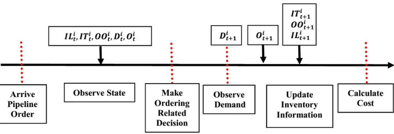
The general mechanism for the sequence of events including arriving pipeline order, observing the system state, making decision about the order, observing demand, and updating the cost, is shown in Figure 1.2. In addition, in each time step 𝑡 of a serial multi-agent system, arriving pipeline order illustrates the demand requested from agent 𝑖, which is equal to the order of the previous agent 𝑖 − 1 with a latency of lead-time LT. This mean that 𝐷𝑡𝑖 = 𝑂𝑡−𝐿𝑇𝑖−1 , if the retailer is the first agent. More details about simulating the environment including different parameters and their relations are given in Tables 1.2 and 1.3 and Chapter 4.
Figure 1.2 The general mechanism for the sequence of events 1.2.1 Type of Inventory Model
Table 1.1 displays the different types of the inventory models. The names of the settings of the models used in the research are made bold and italic. As shown in the table, demand is stochastic, which is selected randomly among one, two, and three, and lead-time is equal to two. Time horizon is set to 500, there is one product, unmet demands are allowed, and there is no limit to capacity. The unrestricted capacity of inventory is one of the benefits of the present research in comparison with the past MDP approaches. The time horizon is reasonably high and its value is chosen by considering working 5 days in every working week for two years (or two times (morning and evening) in every working day of a year). It is assumed that the system does not work for two weeks due to the New Year holiday. The demand and lead-time are the independent Table 1.1 Types of inventory model (The methods written in bold, italic format are used in the present research)
Parameters Type Type Type
Demand Constant Deterministic Stochastic-random(1-3)
Lead-Time “0” “>0” -LT=2 Stochastic
Horizon Single Period Finite (T=500) Infinite
Products One Product Multiple Products -
Capacity Order/Inventory Limits No Limits -
parameters coming from the environments and are the real inputs of DQN. However, since the lead-time is constant, it is not considered as an input parameter. DQN makes decision about ordering-related values as its outputs. The demand is stochastic and is selected randomly among one, two, and three, while lead-time is assumed to be constant equal to two.
1.2.2 DL and RL Components of DRL
In this inventory control problem, the near-optimal long-run cost function consisting of the linear holding, linear backorder, and fixed ordering costs is obtained. This optimization is found by making decision about the ordering value. The inputs are demands during different time steps and the actions are ordering values. The algorithm utilized in this research project is
DQN, whose RL algorithm is Q-learning. Since there is a huge possibility for different pairs of
inputs (demands) and actions (orders), it is impossible to obtain a complete prepared Q-table. Therefore, action selection based on inputs is an online approximation process. The actions of RL are approximated with a DNN. The output of DL is the difference between orders and demands.
Since the present solution is based on RL, “reward” is used instead of “cost” and their concepts are the same in this research. The general goal of DQN is to reduce the long-term cumulative
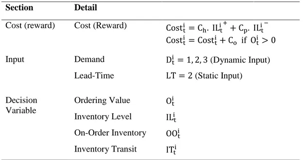
Table 1.2 Components of inventory optimization problem for agent i, time t
(i=1, t<T, T=500)
Section Detail
Cost (reward) Cost (Reward) Cost
t i = C h. ILi +t + Cp. ILi −t Costti = Cost t i + C o if Oti > 0
Input Demand Dti = 1, 2, 3 (Dynamic Input)
Lead-Time LT = 2 (Static Input) Decision Variable Ordering Value Oti Inventory Level ILit On-Order Inventory OOti Inventory Transit ITti
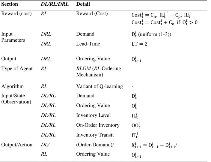
cost (reward) of the agent where the cost of the agent at each time is defined in Table 1.2. The relations between the parameters are presented in Chapter 4. Also, Table 1.2 defines the inventory optimization problem, while Table 1.3 illustrates input/output of DRL as well as the different sections of DL and RL. Since the RL makes decision about ordering, it is a Reinforcement Learning Ordering Mechanism (RLOM). The reward function, state, and action are three main components determining RL and given in Table 1.3. For instance, inventory level is one of the components of each state of RL algorithm, while it is one of the parts of each input of DL. It should be mentioned that although the lead-time is equal to a constant value in all the case studies under study in this research, it can be any positive integer. Since the values of parameters are related to the previous time steps, it will be shown that instead of considering one time step of each parameter, a frame with size 𝑘 of the parameters gives the real ones. The details
Table 1.3 Different sections of DRL and its RL and DL sections for agent i, time t
(i=1, t<T, T=500)
Section DL/RL/DRL Detail
Reward (cost) RL Reward (Cost) Cost
t i = C h. ILi +t + Cp. ILi −t Costti = Cost t i + C o if Oti > 0 Input Parameters DRL Demand Dti (uniform (1-3)) DRL Lead-Time LT = 2
Output DRL Ordering Value Ot+1i
Type of Agent RL RLOM (RL Ordering
Mechanism)
-
Algorithm RL Variant of Q-learning -
Input/State (Observation) DL/RL Demand Dti DL/RL Ordering Value Oti DL/RL Inventory Level ILit DL/RL On-Order Inventory OOti DL/RL Inventory Transit ITti Output/Action DL/ RL (Order-Demand)/ Ordering Value Xt+1i = O t+1 i − D t+1 i / Ot+1i
and relations between decision variables are described in Chapter 4. All of the parameters in Tables 1.2 and 1.3 are previously defined. In addition, 𝐼𝐿𝑖 +𝑡 / 𝐼𝐿
𝑡
𝑖 −shows the inventory level if it is
larger/lower than zero and the absolute value of 𝐼𝐿𝑖𝑡 is considered in the cost function. The
formulae of updating the dependent parameters are presented in the following chapters. 1.3 Contributions
The contributions of the present research work are listed as follows:
The algorithm is designed for an unlimited range of the values of the individual information, while as far as the literature reveals, there are some limitations on the range of individual information such as inventory level for most of the available MDP models. In addition, there is no need to know the input distribution, whereas in the most of the previous works, the demand distribution is required to be known a priori. Also, lead-time related parameters such as on-order inventory and inventory transit are considered. Moreover, the influences of different values of hyperparameters on the performance are examined. Finally, the performance of DQN method is compared with <s,S> and <R,Q> policies and linear regression RL method.
1.4 Thesis Structure
This thesis comprises five chapters which are briefly described below:
Chapter 1 explains the motivation and objectives, problem statement, and major contributions of the present research and outlines the thesis scope. Chapter 2 is devoted to reviewing previous studies for inventory control. Chapter 3 describes theory and formulations related to the research area of inventory management. Chapter 4 is allocated to the proposed methodology adopted herein to solve the problem. It also discusses the results. Finally, Chapter 5 presents a summary and the main conclusions of the present research. It also proposes some suggestions for future works in this filed.
CHAPTER 2
A REVIEW OF INVENTORY CONTROL
A MDP is a formal way to describe the sequential decision-making problems observed in RL.
MDP is not only tractable to solve but is also relatively easy to specify as it assumes to have
perfect knowledge of state. All required information to complete the final task is available in fully observable environments. On the other hand, Partially-Observable Markov Decision Processes (POMDP) act uniformly with all sources of uncertainty. Information gathering actions are permitted in POMDP and yet solving the problem optimally is often highly intractable.
In the field of inventory optimization, there is a number of research works based on a MDP. Van Roy et al. (1997) presented a viable approach based on Neuro-Dynamic Programming (NDP) to solve inventory optimization including a retailer. They formulated two dynamic programming studies containing 33 and 46 state variables. Since the state-space of DP models was large, they could not apply classical DP approaches. Therefore, they implemented the approximate dynamic programming method to simulate this approximation with a Neural Network (NN). Their method falls into the class of NDP techniques. The efficiency of their results was assessed by comparing to S-type policies. Moreover, they examined the reduction in the average inventory cost. The results showed that their optimal control technique provided a reward of about ten percent lower than the reward obtained by heuristic methods. Their research has several restrictions on some parameters such as the number of states and the capacity of inventory. Also, Sui et al. (2010) proposed a RL approach to find a replenishment policy in a vendor management inventory system with consignment inventory. They did not consider the ordering cost and also divided the state space into 50 regions. In contrast, in this research, the ordering cost is included and the real state is studied.
There is a number of RL research studies in the field of inventory control designed for the beer game, which is a serial supply chain network containing (mostly) four agents (stages). The game has a multi-agent, decentralized, independent learner, and cooperative Artificial Intelligence (AI) environment considering holding and back-order costs. No ordering cost is calculated in the beer game whose optimal solution results from a base-stock policy. The game was initially introduced by a group of faculty members in Sloan School Management at Massachusetts Institute of Technology in order to show the difficulty with managing dynamic systems. This game is a
sample of a dynamic system in supply chain which delivers beer from a beer producer to the end customer. Although supply chain structure and rules of playing the game are very simple, the complex behavior of this dynamic system is interesting. The game is categorized in a group of games illustrating bullwhip effect (Devika et al. 2016, Croson and Donohue 2006). This effect happens unintentionally whenever seeking minimum cost. It happens when the order variation in upstream moving node increases in the network. Lee et al. (1997) and Sterman (1989) explained some rational and behavioral causes of the occurrence of the aforementioned effect, respectively. There is no algorithm to find optimal base-stock levels whenever a stock-out is observed in a non-terminal agent. Sterman (1989) analyzed the dynamic of environment by considering the dynamic of stock system and the model of environment flows in the beer game. One of the main points of the game is that no data sharing, which can be inventory value or cost amount, happens until the end of the game. Therefore, each agent has a partial information about environment, which leads to observing a POMDP model. The cost function used in his work was the summation of linear holding and the stock-out (backorder) cost whose coefficients are 0.5 and 1, respectively. This ratio is used in Case Study 2 of the present research.
Giannoccaro and Pontrandolfo (2002) presented a method to find the best decisions about inventory management containing Markov Decision Processes (MDP) and an AI method (RL approach) to solve MDP. Their game consisted of 3 agents whose shipment time and lead-time were stochastic. The RL approach was applied in order to find a near-optimal inventory policy based on maximizing the average reward. The reason for applying RL was due to its stochastic property as well as its efficiency in large-scale networks. Giannoccaro and Pontrandolfo’s RL methods contained three agents whose inventory levels were state variables discretized into 10 intervals and the action number could be between one and thirty. Their methods needed to discretize the inventory level into ten intervals, while it was not generally possible to find an appropriate division of time intervals. This is a defect, which is overcome in this research. Kimbrough et al. (2002) recommended an agent-based approach for serial multi-agent so as to track demand, delete the Bullwhip effect, discover the optimal policies which were known, and find efficient policies under complex scenarios where analytical solutions were not known. Their method was a Genetic Algorithm along with a Joint Action Learners (JALs). They used "𝑥 + 𝑦" rule, in which "𝑥" refers to the amount of demand or order and based on this amount, order
quantity equals "𝑥 + 𝑦". By applying this rule, track demand was carried out and the bullwhip influence was eliminated. This resulted in discovering the optimal policies when these policies could be found. In order to determine the order quantity, Chaharsooghi et al. (2008) proposed an approach similar to the method of Kimbrough et al. (2002) containing two differences. First, they worked with four agents, and second, each game had a fixed length equal to 35 time periods and their state variable consisted of four inventory positions which were divided into nine different intervals. The inventory levels and time intervals were restricted to 4 and 35, respectively, which was a limitation to generalize the work. This problem is resolved in the present research.
Claus and Boutilier (1998) utilized (a simple form of) Q-learning to solve cooperative multi-agent environments. The effect of different features on the interaction between equilibrium selection learning techniques and RL techniques was investigated. They mentioned that Independent Learners (ILs) and Joint Action Learners (JALs) were two different types of Multi-Agent Reinforcement Learning (MARL). A classic type of Q-learning ignoring the other agents was applied in ILs. On the other hand, JALs learned their action value of related agents by combining RL methods with equilibrium learning methods. Parashkevov (2007) evaluated JALs in stochastic competitive games. His approach was able to obtain the safety value of the game and adapt to changes in the environment.
There are two different solutions for the beer game when special conditions arise. In case of availability of stock-out cost only at the final agent (retailer), Clark and Scarf (1960) presented an algorithm to find the optimum policy for the game as the first solution. In order to determine the optimal policy, Chen and Zheng (1994) and Gallego and Zipkin (1999) suggested a similar approach based on the division of serial network into several single-stage nodes. They defined a convex optimization problem with just one variable at each of these stages. Their method suffered from large-volume calculations of numerical integration as well as huge cost of implementation. Later, Shang and Song (2003) proposed an effective approach based on heuristic methods. The solution of Clark and Scarf (1960) and their followers need to consider the specific data distribution, while there is no need to know the data distribution in the present work.
A stochastic process with fixed joint probability distribution is called a stationary environment. If there is no ordering cost and the environment is stationary, the optimal policy of the beer game is
base stock. As Gallego and Zipkin (1999) defined, in this policy, the ordering amount was equal to the difference between a fixed number and the current inventory position. Clark and Scarf (1960) called this constant number a base-stock level and there was no general solution to find the optimal value of the base-stock level when there existed a stock-out cost in any agent except for the final agents (retailers). Gallego and Zipkin (1999), as well as Cheng and Zheng (1994), found optimal solutions by neglecting the stock-out cost. Accordingly, the review of the literature signifies that no definite algorithm was presented when general stock-out was available.
Sterman (1989) presented some relations in order to find the order amount by considering order backlog, in and out shipment flow, on-hand inventory, and expected demand, known as the second solution. He modeled the reactions to shortage or extra inventory value of a four-part serial inventory network. Then, Croson and Donohue (2006) studied the behavioural causes of the bullwhip effect and the subsequent behaviour of the beer game. Recently, Edali and Yasarcan (2014) provided a mathematical model for the game.
Classical supervised ML algorithms such as support vector machine, random forest, or supervised
DNN are inapplicable in this research because of none-availability of historical pairs of
input/output data. On the other hand, the present research is designed based on DQN. Although this research study implements the DQN method into a single-agent model, it can be designed for multi-agent inventory whose agents are JALs and POMDP. The agents roughly work similar to the beer game. One difference is that the parameters such as inventory level are unlimited and there is no restriction on their values. Another difference is that the ordering cost is considered by adding the cost per order to the cost function. To the best of the author’s knowledge, there are limitations on the values of some parameters such as inventory level as well as ignoring ordering cost in most of the past RL approaches. Also, there is a number of research works to solve the one-agent MDP whose parameter values are limited such as inventory capacity. As far as the literature reveals, this is the first work considering the holding, backorder, and ordering costs without any limitation on the values of parameters such as inventory level and without any need to know the demand distribution. Also, in the previous MDP studies, lead-time and its related parameters such as on-order inventory or inventory transit are ignored, while they are considered in the present research study.
CHAPTER 3
THEORY AND FORMULATION
In this chapter, some techniques including RL, DP, and DQN are described and compared. The formulation and details of different techniques including DQN are studied.
3.1 Reinforcement Learning
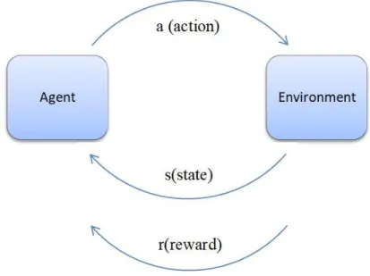
One of the best methods to deal with complicated decision making issues is Reinforcement Learning (RL) (Sutton and Barto 1998). RL is part of Machine Learning (ML) acting with agents whose next status is influenced by action selection. This selection is examined in order to maximize/minimize the future reward/cost by interaction of the agent and the environment.
Figure 3.1 Interaction of agent with environment 3.2 Markov Decision Process
A Markov Decision Process (MDP) is defined as 𝑀 = (𝑆, 𝐴, 𝑃, 𝑅), where 𝑆 is a set of states, 𝐴 is a set of actions, P(𝑆 × 𝑆 × 𝐴 → [0, 1]) is transition probability distribution, and 𝑅(𝑆 → 𝑅) is reward. To be more precise, in each time step 𝑡, a state is the situation of agent and action 𝑎𝑡 is a command in order to reach next state 𝑠𝑡+1 from the current state 𝑠𝑡 by following the state policy π(s). Generally, policy π is a behaviour function choosing actions given states (𝑎 = π(s)) and the transition probability, P(𝑠𝑡+1 = s′|𝑠𝑡 = s, π(s) = 𝑎), shows the probability of transition from
state 𝑠 to state s′ by taking action 𝑎. The general goal of RL is to maximize the expected discounted sum of the rewards over running on an infinite time horizon (Eq. (3-1)).
𝐺𝑡 = 𝑟𝑡+1+ γ𝑟𝑡+2+ γ2𝑟
𝑡+3+ ⋯ = ∑ γ𝑘𝑟𝑡+𝑘+1 ∞
𝑘=0
(3-1)
where γ is the discount factor. However, in case of large state-space and long-running time of RL approach, P and R are very large and are not previously known while the system is a MDP observing the states and rewards after taking an action. The value of a policy is determined by solving a linear system or by doing an iteration which is similar to value iteration. Finding the optimal policy with unknown P and R is a challenging task.
3.3 Comparison of Different Techniques
In order to better understand different approaches, comparisons have been made in this section. 3.3.1 Reinforcement Learning versus Supervised Learning
Supervised Learning is able to solve many problems containing image classification and text translation. However, supervised learning is unable to play a game efficiently. For instance, a dataset containing the history of all the cases of “Alpha-Go” game played by humans could potentially use the state as input x and the optimal decisions taken for that state as output labels y. Although it would be a nice idea in theory, in practice some drawbacks exist as follows:
1. The above-mentioned data sets do not exist for the entire domain.
2. It might be expensive and unfeasible to create the above-mentioned data sets.
3. The method learns to imitate a human expert instead of really learning the best possible policy.
RL wants to learn actions by trial and error. The objective function of a RL
algorithm, 𝐸(∑ 𝑟𝑒𝑤𝑎𝑟𝑑𝑠), is an expectation of a system which is unknown. In contrast, supervised learning algorithms tend to find 𝑚𝑖𝑛𝛳𝑙𝑜𝑠𝑠 (𝑥𝑡𝑟𝑎𝑖𝑛, 𝑦𝑡𝑟𝑎𝑖𝑛), in which 𝛳 shows the parameters of the algorithm and (𝑥𝑡𝑟𝑎𝑖𝑛, 𝑦𝑡𝑟𝑎𝑖𝑛) are pairs of training set. The supervised learning
algorithms learn the optimal strategy by sampling actions and then observing which one of the actions leads to the target output. Contrary to the supervised approach, learning the optimal action in RL approach is not conducted based on one label, rather based on some time-delayed labels called rewards, which then determine the performance of the action. Therefore, the goal of RL is to take actions in order to maximize reward.
A RL problem is described as a Markov decision process which is memory less so that every parameter should be known from the current state. Supervised learning learns by examples of pairs of desired inputs and outputs, while RL learns by agents and guesses the correct output. RL receives some feedback from the quality of its guess, whereas it does not mention whether this output is the correct one and there is probably some delay in seeing the feedback. RL learns either by exploration or by trial and error. The three basic problems in the area of RL are the curse of dimensionality, learning from interaction, and learning with delayed-consequence.
3.3.2 Reinforcement Learning versus Dynamic Programming
Dynamic Programming (DP) is not the same as value or policy iteration conceptually. This is because the DP approaches are the planning methods, which means that they are able to calculate the value function and an optimal policy iteratively by the given transition and a reward function. Dynamic programming is a series of algorithms that can be utilized to calculate optimal policies if the whole model of environment is available as a Markov Decision Process (MDP).
Although classical DP algorithms are less beneficial in RL due to assume a complete model and to be computationally expensive, they are still important from a theoretical standpoint. DP needs a full description of the MDP, with known transition probabilities and reward distributions that are used by a DP algorithm. This property makes it model-based. DP is one part of RL which is a value-based, model-based, bootstrapping and off-policy algorithm. In summary, DP is a planning method, which means that a value function and optimal policy is computed by giving a transition and calculating a reward. On the other hand, Q-learning, which is a special case of value iteration, belongs to a model-free class of RL methods due to not utilizing any environmental model. However, model-based methods work based on learning a model, while contrary to the model-free approaches, the samples are kept even after value estimation. The RL methods try to reconstruct the transition and reward in order to have better efficiency. A
combination of model-free and planning algorithms is presented in model-based algorithms in which fewer sampling is required in comparison with model-free algorithms such as Q-learning. Also, the model-based RL algorithms do not need a model similar to DP approaches such as value or policy iteration. Therefore, fewer sampling and independence from DP modeling are advantages of model-based RL algorithms in comparison with model-free and classical dynamic programming approach, respectively.
3.3.3 Q-learning versus DQN
Q-Learning is one of the pioneer RL approaches presented by Watkins (Watkins and Dayan 1992) and is applied as a baseline of RL results. Although the Q-Learning approach is a powerful algorithm, it is not applicable in all cases. This is because it requires to know all pairs of states and actions while is generally impossible. Therefore, to tackle this problem, an approximation of Q-function can be found by a NN and if NN is replaced by DNN as an action approximator, the algorithm is DQN. This algorithm was introduced by the DeepMind company in 2013 and states and Q-value of the actions were its inputs and outputs, respectively.
The general formula for a Q-function is given as:
Q(s, a) = r + γ maxa′(Q(s′, a′)) (3-2) and the general formula for DQN is
Q(s, a; ϴ) = r + γ maxa′(Q(s′, a′; ϴ̅)) (3-3) In the above formulae, 𝑟 and γ are reward and discount factor, 𝑠, 𝑠′, 𝑎, 𝛳 and 𝛳̅ are state, next state, action, parameters of NN, and parameters to compute the target of NN, respectively.
On the other hand, in DQN, a neural network is added to a very large Q-table in which there is a large number of states and actions. The neural network is applied in order to compress the Q-table by setting the parameters of neural networks. Also, since the number of NN nodes is supposed to be constant, these parameters are restricted to coefficient weights of neural network. By smart tuning the configuration parameters of the structure explained, an optimal Q-function can be found by various neural network training algorithms. If 𝑓𝛳 is a neural network with weight parameters 𝛳 and input 𝑠, the Q-function can be written as 𝑄(𝑠, 𝑎) = 𝑓𝛳(𝑠).
A Q-learning environment contains reward and observation and gives them to an agent in order to decide an action. In DQN, the agent is replaced with a function showing the weights of a DNN. A
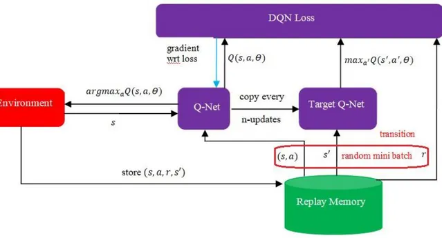
DRL approach learns a parameterized function 𝑓𝛳; its loss function is differentiable with respect to 𝛳 and optimization is performed with gradient-based algorithms. Also, a difference between the Q-learning and DQN is presented in Figure 3.2. 𝛳 is a set of features of neural networks (if the number of nodes and layers in general structure of DNN are considered constant, 𝛳 is considered coefficient weights). Also, 𝑠 and 𝑎 show state and action, respectively.
Figure 3.2 Q-learning (Left) versus DQN (Right) 3.4 Different Types of Reinforcement Learning Algorithms
Model-based and model-free are two different types of RL techniques. The model-based agent builds a transition model of the environment and plans (e.g. by lookahead) using the model. In the model-based algorithms, if there are sufficient samples of each state parameter, the estimations of reward and transition probability converge to the correct MDP, value function and policy. However, obtaining a sufficient number of samples is still a challenge to be solved. A drawback of the model-based method is that the actual MDP model should be made when the size of state is too large. In addition, a policy-based RL approach searches directly for the optimal policy 𝜋∗ which is the policy achieving maximum future reward. Also, value-based RL approach estimates the optimal value function 𝑄∗(𝑠, 𝑎), which is the maximum value achievable under any policy.
The agents of the model-free algorithms such as Q-learning and policy gradient can learn action and policy directly. In addition, a policy-based reinforcement learning approach searches directly for the optimal policy 𝜋∗ which is the policy achieving maximum future reward. Also,
value-based RL approach estimates the optimal value function 𝑄∗(s, a) which is the maximum value achievable under any policy. Temporal Difference (TD), State-Action-Reward-State-Action (SARSA), and Q-learning are some examples of model-free RL algorithms working based on temporal difference. The main benefit of model-free RL approaches is the application of function approximation in order to represent the value function without having to derive. If function approximation with parameters 𝜃 is expressed as 𝑓𝛳(𝑠), TD update is 𝜃 ← 𝜃 + 𝛼(𝑟 +
𝛾𝑓𝛳(𝑠′) − 𝑓𝛳(𝑠))𝛻𝛳𝑓𝛳(𝑠), where 𝑠′ is the next state, 𝛻𝛳𝑓𝛳(𝑠) is the gradient of 𝑓𝛳(𝑠), 𝛼 is
learning rate and γ is discount factor. This process is similar in SARSA and Q-learning. 3.4.1 Q-learning
Q-learning is a model-free approach learning task that applies samples from the environment. It is also an off-policy algorithm due to learning with a greedy strategy 𝑎 = 𝑚𝑎𝑥𝑎 𝑄(𝑠, 𝑎) and it
guarantees sufficient exploration of states due to following a behaviour distribution. This behaviour distribution is chosen by using a ϵ- greedy algorithm, which will be explained in the subsequent sections. Q-function is the main part of Q-learning. 𝑄(𝑠, 𝑎) determines the maximum discounted future reward by performing action 𝑎 when the current state is s. It also estimates the selection of action 𝑎 in state 𝑠. However, “Why is Q-function useful?” and “How is Q-function obtained?” are two main questions worth answering. To achieve this, it is better to see the structure of Q-function. If a strategy to win a complex game is unknown, the players cannot play well. However, the situation is different when a guide book containing hints or solutions is available. The Q-function is similar to this guidebook. If a player is in state 𝑠 and there is a need for action selection, the player selects the action obtaining the highest Q-value. 𝜋(𝑠) is the action associated with state 𝑠 under policy 𝜋 given as:
π(s) = argmaxa Q(s, a) (3-4)
Total future reward is 𝑅𝑡 written as:
Rt = ∑ ri
n
i=t
(3-5) in which 𝑟𝑖 is the reward for each state.
Since the environment is stochastic, there is uncertainty about future increases during running time steps. As a result, calculation of 𝑅𝑡 is not possible, and consequently, discounted future reward is calculated instead of 𝑅𝑡 as follows:
Rt= rt+ γrt+ ⋯ + γn−trn (3-6)
As mentioned previously, the Q-function is the maximum discounted future reward in state 𝑠 and action 𝑎 expressed below:
Q(st, at) = max Rt+1 (3-7)
Therefore, the Q-function can be expressed as the summation of reward 𝑟 and maximum future reward for next state 𝑠′ and action 𝑎′ as follows:
Q(s, a) = r + γ ∗ maxa′Q(s′, a′) (3-8)
This equation is known as Bellman equation. Q-function is solved with an iterative method using an experience (𝑠, 𝑎, 𝑟, 𝑠′). Considering 𝑟 + 𝛾 ∗ 𝑚𝑎𝑥𝑎′𝑄(𝑠′, 𝑎′) as an estimator and 𝑟 + 𝛾 ∗ 𝑚𝑎𝑥𝑎𝑄(𝑠, 𝑎) as a predictor, making a Q-table similar to performing a regression. The loss
function of Q-learning is a Mean Squared Error (MSE) given by: ℒ = [r + γ ∗ maxa′Q(s′, a′) − Q(s, a)]2 ← − − target − −→
← − − − − −TD error − − − −→ (3-9)
Optimization of Q-function with an experience (𝑠, 𝑎, 𝑟, 𝑠′) is performed by considering the
smallest MSE as loss function. If ℒ tends to decrease, the convergence of Q-function to optimal value occurs.
3.4.2 From RL to DQN
The RL techniques are divided into two categories: Tabular Solution Methods and Approximate Solution Methods (Sutton and Barto 1998; Sutton and Barto 2018). If the probability and the reward of transition from state 𝑠 to state 𝑠’ by taking action 𝑎 are given, optimal policy could be found by linear programming or by a type of dynamic programming method such as value
iteration or policy iteration. In most cases, the process is not completely Markov Decision Process (MDP), meaning that the history is somehow important, and as a result, a Semi Markov Decision Process (SMDP) exists. This means that in a system with reasonable running time, in the cases of large state-space and large action-space, finding the optimal policy to solve the MDPs is not possible due to curse of dimensionality. In contrast, in the cases with a large number of states or action spaces, observing full state spaces is not possible for decision makers (agents). This leads to partial observability of state variables called Partial Observable MDP (POMDP). Since it is hard to determine the appropriate Q-values in a POMDP, the approximation of Q-values is made in the Q-learning algorithm (Sutton and Barto 2018). To end this, first, linear regression was used as a function approximator (Melo and Ribeiro 2007), which was replaced by a non-linear function approximator such as neural network due to its ability to find more reliable accuracy. To utilize function approximation, it was necessary to extract a number of features until the early 2010’s. For instance, object recognition methods employed hand-made features and linear classifier learners (Patel and Tandel 2016). However, from 2012, most of vision techniques started utilizing DNN for feature extraction and going towards end-to-end whole pipeline optimization (Szegedy et al. 2013). DL is very successful in learning when the features are unknown. As a result, a combination of RL and DL called DRL has received much attention recently (Li 2017). Mnih et al. (2013) proposed an algorithm for DRL called DQN in 2013. Since 2013, many researchers have worked on this issue and the algorithm is ameliorated and completed significantly (Li 2017). However, the algorithm was not widely used by researchers until the DeepMind group released more details of their approach in 2015 (Mnih et al. 2015). This is because they encountered some difficulties such as observing unstable or even divergent Q-value as Q-function approximator resulting from non-stationary and correlations in the sequence of the observations so as to implement neural network (Mnih et al. 2013). To overcome the challenge, they used the Experience Replay (ER) first introduced by Watkin and Dayan (1992). Schaul et al. (2015) ameliorated their previous research work (Mnih et al. 2015) using the prioritized ER technique. Traffic light control in vehicular networks is its application in transportation (Liang et al. 2018).
3.4.3 DQN
DQN is a combination of Q-learning and Neural Network (NN), in which the function
approximation of Q-learning is a DNN. DQN is a Q-learning approach whose action is chosen based on a DNN. Actions are related to the outputs of NN, whereas states of the RL are the inputs of NN. Also, DQN learns a Q-function by minimizing Temporal Difference (TD) errors. A transition (𝑠, 𝑎, 𝑟, 𝑠′) is observed and TD error tends to make 𝑄(𝑠, 𝑎) as close as possible to 𝑟 +
𝛾𝑚𝑎𝑥𝑎′𝑄(𝑠′, 𝑎′). Action can be selected arbitrarily in off-policy algorithms with a ϵ-greedy policy based on the current Q-value. To be more precise, value function 𝑄𝜋(𝑠, 𝑎) is the expected total reward from state 𝑠 and action 𝑎 under policy 𝜋 which can be unrolled recursively as follows:
𝑄𝜋(𝑠, 𝑎) = 𝔼[𝑟𝑡+1+ γ𝑟𝑡+2+ γ2𝑟𝑡+3+ ⋯ |𝑠, 𝑎] = 𝔼𝑠′[ r + γ 𝑄𝜋(s′, a′)|𝑠, 𝑎] (3-10) Also, optimal value function 𝑄∗(𝑠, 𝑎) can be unrolled recursively as:
𝑄∗(𝑠, 𝑎) = 𝔼𝑠′[ r + γ 𝑚𝑎𝑥𝑎′ 𝑄∗(s′, a′)|𝑠, 𝑎] (3-11) where value iteration algorithms solve the Bellman equation as follows:
𝑄𝑖+1(𝑠, 𝑎) = 𝔼𝑠′[ r + γ 𝑚𝑎𝑥𝑎′ 𝑄𝑖(s′, a′)|𝑠, 𝑎] (3-12)
The value function represented by deep Q-network whose parameters are 𝜃 is given by:
𝑄(𝑠, 𝑎, 𝜃) ≈ 𝑄𝜋(𝑠, 𝑎) (3-13)
The objective function defined by mean-squared error in Q-values is expressed as: ℒ = 𝔼[(r + γ ∗ maxa′Q(s′, a′, 𝜃̅) − Q(s, a, θ))2]
← − − target − −→
← − − − − − − TD error − − − −−→
(3-14)
which leads to the following gradient function: ∂ℒ(θ)
∂θ = 𝔼[(r + γ ∗ maxa′Q(s
′, a′, 𝜃̅) − Q(s, a, θ)]∂Q(s, a, θ)
∂θ
As a result, the end-to-end RL is optimized by an optimizer using ∂ℒ(θ)
∂θ .
3.4.4. Optimizers
There are many optimizer techniques among which Stochastic Gradient Gdescent (SGD) and ADAptive Moment estimator (ADAM) are more favorite. The batch methods utilize the entire training sets in order to update the parameters in any iteration with a tendency to converge to local optimal. For a large dataset, the speed of finding the cost and gradient of the full training data set is very low. Also, a batch optimization approach is not a suitable method to merge new data in the online settings. In order to resolve these problems, SGD approaches follow the negative gradient of objective after a few training samples. Since the cost of the running backpropagation over the entire training set is high, it is helpful to use SGD in neural network setting. In SGD, the parameters 𝛳 of objective 𝐽(𝛳) are updated with 𝛳=𝛳− 𝛼𝛻𝛳𝐸[𝐽(𝛳)], where 𝛻𝛳 is the gradient of 𝛳 and 𝛼 is the learning rate. If SGD uses a few training samples, it easily disappears with the update expectation and gradient computation. As a result, the update is given by a new formula extracting (𝑥(𝑖), 𝑦(𝑖)), where 𝑥(𝑖) and 𝑦(𝑖) are the 𝑖𝑡ℎ pair of training set,
from the training data as follows:
ϴ=ϴ− α∇ϴJ(ϴ; x(i), y(i)) (3-16)
Updating the parameters in SGD is based on a few trainings or mini-batch samples. This is due to variance reduction in the updated parameters, leading to a more stable convergence. Also, it can benefit from the optimized matrix operations used in computation of cost and gradient. The learning rate of stochastic gradient descent, 𝛼, is lower than that of batch gradient descent due to the existence of more updating variance. The decisions are made to find the correct learning rate and time of updating the learning value.
Also, Adaptive Moment Estimation (Adam) computes the adaptive learning rates of each parameter which not only stores an exponentially decaying average of past squared gradient 𝑣𝑡, but also keeps an exponentially decaying average of past gradients 𝑚𝑡 which is similar to momentum. Adam behaviour is similar to heavy ball with friction which prefers to flat minima in the error surface, whereas momentum pushes a ball running down a slope. 𝑚𝑡 and 𝑣𝑡 estimate the