HAL Id: hal-02699185
https://hal.inrae.fr/hal-02699185
Submitted on 1 Jun 2020
HAL is a multi-disciplinary open access
archive for the deposit and dissemination of sci-entific research documents, whether they are pub-lished or not. The documents may come from teaching and research institutions in France or abroad, or from public or private research centers.
L’archive ouverte pluridisciplinaire HAL, est destinée au dépôt et à la diffusion de documents scientifiques de niveau recherche, publiés ou non, émanant des établissements d’enseignement et de recherche français ou étrangers, des laboratoires publics ou privés.
NOAA/AVHRR satellite measurements
Sophie Moulin, L. Kergoat, Nicolas Viovy, G. Dedieu
To cite this version:
Sophie Moulin, L. Kergoat, Nicolas Viovy, G. Dedieu. Global-scale assessment of vegetation phenology using NOAA/AVHRR satellite measurements. Journal of Climate, American Meteorological Society, 1997, 10 (6), pp.1154-1170. �10.1175/1520-0442(1997)0102.0.CO;2�. �hal-02699185�
q 1997 American Meteorological Society
Global-Scale Assessment of Vegetation Phenology Using NOAA/AVHRR Satellite
Measurements
S. MOULIN, L. KERGOAT, N. VIOVY,*AND G. DEDIEU
Centre d’Etudes Spatiales de la Biosphe`re (CNES/CNRS/UPS), Toulouse, France
(Manuscript received 18 April 1995, in final form 9 September 1996) ABSTRACT
Phenology and associated canopy development exert a strong control over seasonal energy and mass exchanges between the earth’s surface and the atmosphere. Satellite measurements are used to assess main phenological stages of the vegetation at the global scale. The authors propose a method to derive the start, the maximum, the end, and the length of the vegetation cycle, based on the analysis of temporal series of weekly vegetation index, at a resolution of 18 lat 3 18 long for year 1986. Global maps of these characteristics of the vegetation are presented, and their zonal distribution is discussed. The start of the vegetation cycle has been related to temperature sums in the case of temperate deciduous forest and to precipitation in the case of savannahs. It is concluded that satellite measurements offer interesting perspectives for global-scale quantitative phenology modeling.
1. Introduction
Current needs to model and predict interactions be-tween biosphere and climate in terms of energy, mass, and momentum exchange at the land surface–atmo-sphere interface have led to dedicated field experiments [e.g., the First Field Experiment (FIFE), see Sellers and Hall (1992); and the Hydrological Atmospheric Pilot Experiment, see Andre´ et al. 1988; Goutorbe et al. 1994], which provide opportunities to develop and test models at different scales. Canopy-scale modeling and up scaling problems have been addressed through dif-ferent approaches [Garratt (1993) reviewed surface schemes in use in climate models; Raupach (1995), among others, discussed up scaling methods]. These ex-periments have also demonstrated the importance of long-term time series (at least 1 yr) and corresponding models. At this timescale, the seasonal rhythm of the vegetation exerts a strong control over surface–atmo-sphere interactions. For instance, senescence of above-ground tissues results in a large decrease of the latent flux and corresponding increase of the sensible heat flux, over the FIFE tall grass prairie (Verma et al. 1992; Fritschen and Quiang 1992). Conversely, the develop-ment of the leaves surface generally increases the
can-*Additional affiliation: Laboratoire de Mode´lisation du Climat et de l’Environnement (CEA/DSM), Gif sur Yvette, France.
Corresponding author address: Dr. Sophie Moulin, CESBIO, 18,
Avenue E. Belin, BPI 2801, Toulouse Cedex 4, France, 31401. E-mail: sophie.moulin@cesbio.cnes.fr
opy conductance (curvilinear relationships) and then plant transpiration (Saugier and Katerji 1991). Surface– atmosphere interactions also involve complex feed-backs, especially when changes in the surface prop-erties, caused by active response of the vegetation to climate forcings are considered. Dirmeyer (1994), for instance, showed that a drought-induced senescence applied to SiB (a simplified version of the Simple Bio-sphere Model; Sellers et al. 1986; Xue et al. 1991) results in an increased severity and decreased duration of the continental midlatitude drought simulated by a GCM. These examples highlight the interest of ob-serving and modeling vegetation seasonal changes.
Over the world and for particular vegetal species, plant phenological observation networks exist (Hopp 1974). Some observations have also been used to in-vestigate the vegetation phenology that is the timing of recurring biological events and their relationships to environmental forcings. For particular plant species, many studies have shown that environmental factors (climatic parameters, soil characteristics, geographic components) are closely associated with plant devel-opment. Nienstaedt (1974) reviewed several studies relative to North American tree species. These studies have demonstrated that temperature plays a major role in the control of phenological response. An important issue concerns the ability to predict the environmental control of the vegetation phenology. Hunter and Le-chowicz (1992) have compared several models of bud-burst prediction based on the response to warming, winter chilling, and photo-period with historical ob-servations, for northern hardwood trees. Murray et al. (1989) measured the thermal times to budburst for
sev-eral woody perennials in different conditions of chill-ing duration. Then, for each species, this thermal time has been fitted to durations of chilling through three-parameter exponential relations. Kramer (1994) has compared different models to predict the onset of growth for beech species. Models were obtained by fitting an onset date–temperature relation to observa-tions. Schwartz and Marotz (1986) compared observed and predicted dates for the arrival of the green wave, for a particular shrub species, over North America. They used both traditional accumulation models, which consider the amounts of sensible heat and solar radi-ative energy, and synoptic model (regression formu-lations; Schwartz 1990). Moreover, Schwartz (1992) showed that midlatitude spring ‘‘green-up’’ and strong changes in surface-level meteorological variables oc-cur at nearly the same time. The phenological infor-mation was based on first-leaf emergence of a Lilac clone Syringa chinensis, for 200 sites of a phenological stations network (Hopp 1974). He further used a ‘‘spring index’’ (Schwartz and Karl 1990), based on similar information for three different species, as an indicator of large-scale vegetation phenology. So phe-nological models, which describe the response of can-opy development to climatic factors, have been de-signed for many different species.
However, biosphere–atmosphere interactions study requires large-scale phenology observation and mod-eling. Space-borne sensors have been used to monitor vegetation at the global scale (e.g., Tucker et al. 1981; Goward 1989). Many studies used AVHRR datasets in order to map the land cover both at continental (Love-land et al. 1991; Love(Love-land et al. 1995; Running et al. 1994) and global (Nemani and Running 1995; Nemani and Running 1996; Brown et al. 1993) scales. Recently, Defries et al. (1995) have derived phenological param-eters, for vegetation mapping purposes. Most of these studies use the temporal information of remotely sensed signal to produce vegetation category maps.
In this study, we derive—from remote sensing and at global scale—phenological characteristics that are re-quired parameters for a terrestrial biosphere model. Justice et al. (1985) first presented a qualitative, global overview of vegetation seasonality and showed the vari-ability in vegetation index response over time associated with vegetation types at continental scale. Recently, Reed et al. (1994) have derived quantitative phenolog-ical parameters, over the United States, for given veg-etation classes. Over African intertropical zone, Fonte`s et al. (1995) compared satellite data to a monthly phe-nological rhythm model describing the biome-specific relationships between bioclimates and vegetation sea-sonality. The comparison between simulated vegetation activity and 10 yr of monthly GVI data shows a simi-larity of temporal patterns.
This paper is an attempt to derive quantitative infor-mation on vegetation phenology, not in terms of struc-ture but in terms of timing. The seasonal behavior of a
18 lat 3 18 long grid cell is characterized by the dates of beginning, end, and maximum of the satellite-derived normalized difference vegetation index (NDVI) season-al cycle. The phenologicseason-al study presented here is per-formed at global scale with a weekly time resolution for phenological stages, whereas most studies are per-formed at local or continental scales with a biweekly or monthly time resolution. The global patterns are ana-lyzed, and we show, for two vegetation types (cold de-ciduous forest and savannah), how phenology can be related to climatic factors (air temperature and precip-itation).
2. Data description a. Satellite measurements
The National Oceanographic and Atmospheric Ad-ministration/Advanced Very High Resolution Radiom-eter (NOAA/AVHRR) sensor, initially conceived for meteorological applications, is a very powerful tool to monitor vegetation (Tucker et al. 1981; Townshend 1994). Its characteristics are a high temporal frequency (daily global coverage), a low spatial resolution (about 1 km 3 1 km), and the presence of both visible and near-infrared (NIR) channels. These properties make it an attractive tool to study the evolution of vegetation at global scale.
The NDVI, computed from visible and NIR reflec-tance factors, characterizes the phenological state of the vegetation (Rouse et al. 1974). NDVI has been related to vegetation activity and to biophysical parameters like fraction of absorbed photosynthetically active radiation. We used global vegetation index (GVI) data, which con-sist of weekly composites at a 0.1448 latitude and lon-gitude resolution (Kidwell 1990; Gutman 1994). Sat-ellite measurements were recorded by NOAA-9 for 1986. A correction was performed for the radiometric gain drift, using post-launch coefficients (Teillet and Holben 1994). Then, corrections for atmospheric effects (ozone, Rayleigh diffusion) were applied through simplified method for atmospheric correction (SMAC) (Rahman and Dedieu 1994) using climatologies for ozone at-mospheric content (London et al. 1976). No correction for water vapor or aerosol effects was performed (see section 4a). We assumed that such effects mainly affect the global dynamics of the signal and not temporal pro-file pattern: cycle phase and duration. Reflectances were averaged to calculate NDVI at 18 lat 3 18 long reso-lution. Despite the physical corrections of the signal and the use of the maximum value composite method on GVI data for cloud screening, temporal profiles were still too noisy to characterize vegetation cycles. There-fore, we used the best index slope extraction filtering method (Viovy et al. 1992) to filter out residual per-turbations, especially cloud contaminated data.
FIG. 1. Description of the detection algorithm of transition dates: NDVI time profile (solid), time profiles of criteria allowing the de-tection of start (dash–dash) and end (dash–dot) dates. Start and end dates (*) were obtained when criteria time profiles are minima.
b. Climate factors
A great number of climatic factors influence vege-tation growth and development (Lieth 1974). Among these parameters, temperature and precipitation are most important in triggering the vegetation growth. Air tem-perature affects plant mechanisms such as respiration, transpiration, and photosynthesis. It strongly depends on solar radiation. We used the evolution of temperature during the year to test the impact of climate on vege-tation seasonal cycle. In temperate and boreal regions, the start of the vegetation growing period is usually related to temperature (e.g., Taylor 1974; Hunter and Lechowicz 1992; Cannell and Smith 1986). Water is also a determinant factor for plant life both in a vapor form in the atmosphere, and in a liquid state, affecting plant physiology and growth process. Annual rainfall and its distribution over the year strongly drive plant development. In tropical dry regions, the beginning of vegetation season is mostly driven by rainfall (e.g., Menaut 1983; Medina 1993; Frankie et al. 1974). Other ecological factors like fire and wind were not consid-ered.
Monthly mean air temperature and precipitation mea-surements, from the weather station network (Spangler and Jenne 1990), have been grided (18 3 18) using a four nearest neighbors linear interpolation. A temporal interpolation (linear) was used to obtain a weekly da-taset.
c. Matthews’s vegetation map (1983)
Matthews’s global vegetation map (1983) is used to illustrate results obtained for two given ecosystems. This classification displays the different types of natural vegetation according to the United Nations Educational, Scientific, and Cultural Organization classification scheme. It is commonly used in the literature, in par-ticular for biogeochemical and climate models (e.g., the FBM, Lu¨deke et al. 1994). Thirty-two classes of veg-etation are classified according to their physiognomic characteristics (lifeform, density, and seasonality) but also to other factors such as altitude, climate, and veg-etation architecture.
3. Method: Determination of transition dates
Viovy (1990) described the evolution of each plant cover type as a succession of states (representing the development stages of the canopy), which can be as-sociated to different phenological stages. To simplify the reality, we consider that the vegetation displays one seasonal cycle or no cycle at all. When the radiometric signal is characterized by a marked main cycle, we as-sume this cycle can be described by three successive periods: ‘‘dormancy,’’ growth, and senescence. Dor-mancy refers here either to real dorDor-mancy or to the off-leave period of deciduous and annual vegetation. On a
NDVI time profile, the three periods are characterized by an evenly low NDVI, which increases until reaching a maximum value and finally decreases. The objective of the proposed method is to detect the time of transition between two states on the NDVI time profile. We did not determine the instantaneous phenological state of the vegetation, but rather the timing of the change from one state to the other, that we called state transition dates.
The three-period simple shape is a reasonable rep-resentation of the behavior of temperate regions trees, and of most tropical biomes. The relevance of the as-sumption will be discussed for biomes like continental grasslands and Mediterranean vegetation. Besides, for tropical rain forest and sparse vegetation, the analysis may be obscured by data contamination (see section 4a).
Description of the detection algorithm
Various algorithms have been developed to detect specific dates from a radiometric signal (e.g., Kaduk and Heimann 1996). The algorithm we used allows us to detect three transition dates: beginning, maximum, and end of the vegetation cycle through the analysis of the NDVI temporal series. Determination of the start and end dates was done by finding the minimum of two criteria calculated for every week (Fig. 1).
1) BEGINNING DATE OF THE CYCLE(BpDATE) The criterion biused to determine the beginning of the cycle (bpdate) is based on the following consider-ations: (i) NDVI value is close to a value of bare soil; (ii) the time derivative before bpdate (left derivative) should be zero, NDVI being almost constant; and (iii) on the opposite, the time derivative after bpdate should
be positive as the signal increases when the vegetation appears. For smoothing purposes, left and right time de-rivatives were computed with xi12, xi22and not xi11, xi21, such that
bi5 zxi2 x0z 2 l[(xi122 xi)2 zxi222 xiz], (1) where biis bpdate criterion for week i (from week 5 to week 50), xiis radiometric signal value for the date i, and x0andl are empirical parameters. As the beginning
of the time series cannot be filtered (boundary effect), the first two values are not significant, so the detection begins on week 5 instead of week 3.
2) DATE OF THE CYCLE END (EpDATE)
The date at which vegetation cycle ends was calcu-lated similarly to the beginning date. The NDVI value must be close to the soil threshold, and the left derivative is negative as the signal decreases during the senescence phase and equals zero on right, such that
ei5 zxi2 x0z 1g[zxi122 xiz 2 (xi222 xi)], (2)
where eiis epdate criterion for week i.
Each equation [Eq. (1) and Eq. (2)] includes a term accounting for the mean level of the signal (‘‘mean term’’) and a term accounting for the shape of the signal (‘‘derivative term’’). A soil threshold (x0) is used
in the mean term of the equation, whereas a slope co-efficient (l or g) is used in the derivative term. Thresh-olds and coefficients used in the algorithm were em-pirically set.
With the mean term, variations of soil color and tex-ture can induce variations of NDVI even if there is no vegetation. Among two dates leading to the same de-rivative term, the mean term helps the algorithm to se-lect the one that has the lowest value (i.e., which is the closest to the soil or constant green background). For pixels covered with bare soil during a part of the year, the mean term Eq. (1) allows us to detect the beginning date of the cycle when the NDVI is close to bare soil threshold. For pixels with a constant background veg-etation (and then a constant level of NDVI always above the soil threshold), the algorithm also detects the be-ginning of the cycle (when the NDVI level is close to, but larger than, the background level). Here, x0
corre-sponds to NDVI values observed for the Matthews (1983) desert class.
For the derivative term, the factors l and g weight the derivative term of Eqs. (1) and (2). Hence, ifl and
g are too large, the algorithm may fail for pixels with
a large part of the year with no vegetation (i.e., arid or cold regions). Indeed, in that case, the detection may be confused by short-term signal variations due to re-sidual noise (e.g., soil color, directional effects). On the other hand, if the values are small, the algorithm may fail for pixels, which remain partly green during the year. According to this,l and g are empirically set to 3 and 5, respectively, in order to obtain a compromise
between the two terms (mean and derivative). Due to the shape of seasonal profiles, the factorg is larger than
l. In fact, for a large number of grid cells, the decrease
of the radiometric signal is slower than the increase. So, the weight of the derivative term must be amplified to detect the ending date.
3) DATE OF THE MAXIMUM MAGNITUDE(MpDATE)
The determination of maximum of the vegetation cy-cle corresponds to the date of the maximum value of the NDVI time series.
4) CYCLE LENGTH
As time series begin arbitrarily in January, cycle length is the difference between epdate and bpdate when bpdate ‘‘precedes’’ epdate. In the other case (Southern Hemisphere), the length is 52–(epdate–bpdate).
Additional rules established to obtain a global-scale detection of transition dates are presented in the appen-dix. They mostly deal with the detection of water sur-faces and of areas where vegetation dynamics does not allows the detection (mainly corresponding to evergreen vegetation and desert area), and finally with areas where solar irradiance is very small a part of the year (austral and boreal regions).
4. Results and discussion: Seasonal cycle and climatic drivers
a. Global-scale results
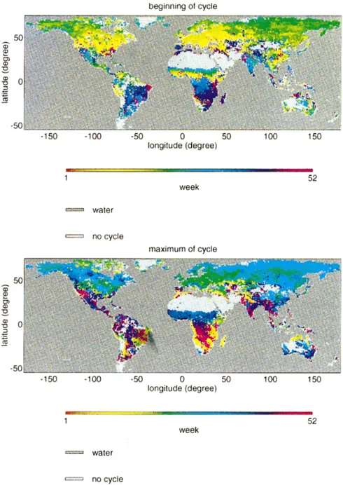
Figure 2 displays maps of dates of the beginning (Fig. 2a), the maximum (Fig. 2b), end of the growing cycle (Fig. 2c), and finally the vegetation cycle length (Fig. 2d). We notice a general spatial homogeneity of dates, which suggests the homogeneity of environmental fac-tors at the corresponding scale. Changes from an eco-system to an other are generally continuous and vari-ations are gradual.
The map of cycle beginnings is spatially rather ho-mogeneous. The ends of cycle (and then the cycle du-rations) are much more speckled than the beginning dates. The increase slope of NDVI profile is often very steep, whereas NDVI decrease slope is not: the time profile is characterized by a progressive return to dor-mancy state. The detection of cycle ends is then very sensitive to small NDVI variations and leads to noisy global maps for cycle end and length.
Differences and similarities exist between the global maps of transition dates and natural vegetation maps. Over the North American continent, the transition be-tween east and west observed on Matthews’s (1983) classification does not appear on phenological maps. Although the type of vegetation and the NDVI intensity are different over each side of the continent, transition dates maps show that phenological behavior does not
FIG. 2. Global-scale maps of vegetation transition dates obtained from 1986 GVI dataset. (a)–(d) Beginning, maximum, end, and length of the vegetation cycle, respectively.
vary from east to west. On the other hand, the contrasted phenology between Northern and Southern Australia agrees with Matthews’ vegetation map (1983). The same correspondence is observed for China and India.
At this coarse scale, crop and natural vegetation areas cannot be clearly distinguished in terms of beginning and end of vegetation cycles. In a square degree pixel, there is always a part of the surface that is covered by natural vegetation.
Figure 3 represents a zonal average of transition dates: for each latitude, date values were averaged over
lon-gitude. Pixels that correspond to water surfaces and aus-tral vegetation, or with insufficient NDVI dynamics (dense forests, desert areas) were not considered. The Northern and Southern Hemisphere Tropics display in-verted temporal phasing. The spring green wave comes from March to May over most of the Northern Hemi-sphere. Over the Southern Hemisphere, the vegetation cycle begins at end of year (which corresponds to the austral spring) and ends the following year. These results apply mostly to the grasslands of South America and to African savannahs.
FIG. 2. (Continued)
1) LATITUDINAL VARIATIONS
The variations of vegetation phenological behavior with latitude is the most striking trend (Figs. 2 and 3).
(i) Northest latitudes
In high-latitude zones (Canada, Greenland), the ex-istence of scattered points is the result of noisy data due to the low solar irradiance (see appendix).
(ii) From 758 to 408N
Over the Northern Hemisphere, the length of the veg-etation cycles regularly decreases when latitude increas-es from temperate to boreal regions (Woodward 1987). The bpdate increases with a rate of about 1 week per degree latitude (Fig. 3). Peak vegetation cycle dates are strikingly similar from 408N to 758N. They correspond to the end of July, about 1 month after summer solstice, and correlates with maximum temperature.
Second-FIG. 3. Zonal average of vegetation transition dates: beginning (*), maximum (1), and end (V) obtained from 1986 GVI dataset. For a given latitude, the average over longitudinal values was performed. Pixels for which the radiometric signal dynamics was too low (see appendix) and austral zones pixels were not taken into account. This latitudinal average was calculated consid-ering that the year is cyclic (the last week of the year is close to the first one). For a given latitude, the average value is plotted only if the variability of transition dates is small; that is, most pixels have comparable time profiles (the average modules is superior to a threshold empirically set at 0.4)
order longitudinal variations, such as orography effects (e.g., Oural mountains) are observed.
(iii) From 408 to 308N
This region is mainly represented by the desert belt (e.g., Gobi and Sahara Deserts) with no vegetation cover.
(iv) From 308 to 108N
For the whole tropical and subtropical region, the NDVI cycle correlates with the monsoon oscillations. As for temperate region, mpdate does not vary and oc-curs in early October. Figure 3 shows a very rapid in-crease of bpdate, which ranges from the end of March at 108N to the end of July at 158N. This is mainly rep-resentative of the Sahelian’’ and ‘‘Sudano-Guinean’’ savannahs of Africa (Fig. 2). The beginning of the vegetation cycle is directly linked to the inter-tropical convergence zone (ITCZ; Kerr et al. 1989). The end of cycle is not represented because of the large longitudinal variation. Over South Asia, the vegetation cycle begins between mid-June and mid-July and is cor-related to the arrival of the monsoon. Figure 2 displays small latitudinal variations. The end of the vegetation cycle occurs during the following year around
mid-March. Due to a very slow decrease in NDVI from the maximum to the end, the vegetation cycle is very long. The nonactive period lasts only 10 weeks. Figure 2a shows the difference of behavior for the same latitude over Asia and China. We also notice a difference be-tween northeast and southwest China in Fig. 2c.
(v) From 58N to 58S
The equatorial belt is dominated by evergreen veg-etation cover (Medina 1983; Frankie et al. 1974). Most of the pixels are classified as ‘‘no cycle’’ (Fig. 2) or display very long cycles. However, the maps present some unrealistic very short cycles.
(vi) From 58 to 408S
A 6-month shift is observed compared with the mon-soon regime of the Northern Hemisphere. An important latitudinal gradient for the maximum of cycle is shown (Fig. 3). For South America, the beginning date does not vary with latitude. The end of the cycle does not vary except in south. There is a dissymmetry in the cycle since the growing period is very short compared to senescence. This leads to very long active periods (e.g., Angola, Zaire, Brazil).
FIG. 4. Monthly mean atmospheric water vapor content. Data re-drawn from Justice et al. (1991) for Gao (16.258N, 0.058W—year 1986), data from Faizoun et al. (1994) for Bidi (15.838N, 2.838W— year 1986), and Oort’s climatology (1983) for a temperate site (38.168N, 96.048E) and a boreal site (66.538N, 96.048E).
FIG. 5. Sensitivity of surface NDVI retrieval to a range of atmo-spheric correction of TOA AVHRR reflectances, for Gao (Mali). [H2O] is the monthly mean of water vapor reported by Justice et al.
(1991),tpis the aerosol optical depth, andtpHis the aerosol optical
depth reported by Holben et al. (1991): 1) top of the atmosphere NDVI (no atmospheric correction); 2) correction of Rayleigh scat-tering, neither aerosol nor gaseous absorption; 3) correction of Ray-leigh scattering, ozone absorption, and aerosol scattering and ab-sorption (constanttpof 0.23 at 550 nm, water vapor5 0.5[H2O]; 4)
correction of Rayleigh scattering, ozone absorption, and aerosol scat-tering and absorption (tp5tpH), with water vapor5 [H2O]; and 5)
correction of Rayleigh scattering, ozone absorption, and aerosol scat-tering and absorption (tp5tpH), with water vapor5 1.5[H2O].
2) REGIONAL PATTERNS
(i) Mediterranean area (see Mooney et al. 1974)
We notice a singular behavior on transition dates maps for the Mediterranean vegetation (e.g., south of Spain and North Africa). Cycles begin in the fall (Sep-tember). Vegetation is greatly stressed during summer [Leaf Area Index (LAI) and then NDVI signal decrease] and begins regrowth with autumn rainfall. This leads to a bimodal cycle, the main growth being observed in spring. During the winter, the temperature remains mild enough to sustain green vegetation.
(ii) Australia
The phenology observed in the south of Australia (from 308S to 408S) is phased with the Northern Hemisphere, as described by Graetz et al. (1995). They observed a shift of about 6 months between sites located in the north and in the south of Australia, with the vegetation mainly driven by rainfall. For the whole Southern Hemisphere, the winter dormancy phenology, which is widespread in the Northern Hemisphere, is confined to South America, New Zealand, and the southern edge of Africa.
3) ALGORITHM AND DATA LIMITATIONS
(i) Atmospheric effects
Seasonal variations of atmospheric characteristics (e.g., Fig. 4) may create an artificial seasonal cycle of NDVI that does not correspond to any actual change of
vegetation or may mask an existing vegetation cycle, especially if the actual surface NDVI is low. Justice et al. (1991) have shown that over the sahelian site of Gao (16.258N, 0.058W), dry season AVHRR NDVI is ele-vated by the reduction of atmospheric water vapor, com-pared to the rainy season, leading to a NDVI cycle that is out of phase with the vegetation cycle.
To illustrate this issue, we show NDVI values re-trieved over this specific site of Gao when atmospheric correction are applied for a range of atmospheric char-acteristics (Fig. 5). We used monthly means of water vapor (March to September 1986) and aerosol optical depth (February to September 1986) reported by Justice et al. (1991) and Holben et al. (1991), respectively. Missing data for water vapor have been derived from Oort’s climatology (Oort 1983). Aerosol optical depth for January (respectively, October to December) was set equal to that of February (respectively September). Ra-diative transfer was simulated with the SMAC method (Rahman and Dedieu 1994), using the GVI solar zenith and view angles. The transition date detection algorithm detects a vegetation cycle only if the maximum ampli-tude of NDVI is greater than 0.06 (see appendix). This is the case when it is applied to top-of-the-atmosphere (TOA) NDVI or to NDVI only corrected for Rayleigh
FIG. 6. Sensitivity of surface NDVI retrieval to a range of atmo-spheric correction of TOA AVHRR reflectances, for Bidi (Burkina Faso). We used monthly means of water vapor content, [H2O], and aerosol optical depth, tpF, reported by Faizoun et al. (1994). The
lowest NDVI values correspond to TOA NDVI and correction of Rayleigh scattering (no aerosol, no absorption). The other plots have been obtained for a range of water vapor content (0.5[H2O], 1.5[H2O]) and aerosol optical depth (0.23,tpF). In every case, the
beginning date (*) is obtained with Eq. (1).
scattering (plot 2 in Fig. 5). This latter case corresponds to the atmospheric correction we applied to GVI data for the global-scale study. When further corrections (e.g., water vapor) are applied, no cycle is detected (cases 3–5). Therefore, atmospheric effects may create artificial NDVI seasonal cycle, particularly at low NDVI [see Tanre´ et al. (1992) for a comprehensive sensitivity study]. This cycle can be probably removed in most cases by correcting for water vapor absorption (e.g., by using water vapor climatology or GCM analysis).
Apart from creating artificial NDVI cycles, atmo-spheric effects could also generate errors on the retrieval of the phenological dates if they are not accounted for properly. To illustrate this issue, we corrected TOA re-flectances acquired over Bidi (Burkina Faso, 15.838N, 2.838W) for a range of atmospheric conditions and com-puted the corresponding ‘‘surface’’ NDVI. We used at-mospheric water vapor content and aerosol optical depths derived from sunphotometer measurements in Bidi in 1987 (Faizoun et al. 1994). Figure 6 presents surface NDVI retrieved for that range of atmospheric corrections. Water vapor content has been varied between
650% (twice the standard deviation) around the
mea-sured monthly mean values, and we used both meamea-sured aerosol optical depths and a constant value oftp5 0.23
at 550 nm. Whatever the water vapor content is, the dates retrieved for the beginning of vegetation cycle (Fig. 6) vary from week 29 fortp5 0.23 to week 31 when the
aerosol optical depth is large (i.e., Faizoun et al. 1994). A more comprehensive study of the effects of the at-mosphere and of their correction on phenology moni-toring is beyond the scope of this paper. However, the
examples discussed here are for regions that exhibit large seasonal variability of atmospheric water vapor, high aerosol content, and low vegetation cover. If we except very cloudy areas, these conditions are probably among the worse than can be found. Noticeably, Fig. 2a shows few reverse cycles for the Sahelian Northern boundary, mainly because atmospheric-created cycles disappear as a result of both the 18 3 18 spatial averaging and thresh-old on NDVI seasonal dynamics. In summary, atmo-spheric effects may introduce bias on phenology retrieval or even create artificial cycles. These errors are partic-ularly important for lowly vegetated areas. Atmospheric corrections are to be applied to improve the quality of the results, but the problem of continuous cloud cover still remains.
(ii) Tropical evergreen forests
Despite the tests used (see appendix), detection of transition dates was performed for some nonvegetation cycles. It is the case over equatorial forests where mea-sured NDVI dynamics is due to residual cloud contam-ination and the detection of any marked cycle (Gutman 1994) is hazardous due to cloud contamination. A more drastic filter might be applied to GVI data to discard these pixels [some studies rebuild a constant temporal NDVI signal to characterize these areas (e.g., Sellers et al. 1994)]. Consequently, results may not be consistent over tropical evergreen forests.
(iii) Boreal regions
The impact of snow on phenology detection over boreal regions was evaluated. In the case of evergreen forests, Spanner et al. (1990) showed that, besides tree growth during spring and summer, the observed growing cycle corresponded to snowmelt (Reed et al. 1994). The detected beginning dates correspond to important and sudden vari-ations of visible reflectances from 0.4 (or more) for snow to 0.14 (or less) for vegetation. This variation of reflec-tances creates a steep increase on NDVI time profile, which is detected by the algorithm. So, in boreal regions, the detected bpdate corresponds to the date of snowmelt.
(iv) Grassland biome
The hypothesis assuming that the radiometric signal can be described by three successive periods (dormancy, growth, and senescence) may not be satisfactory for continental grassland, which may be governed by winter cold determinism, and summer drought determinism (French and Sauer 1974). The LAI decrease during sum-mer due to water stress leads to a multimodal cycle.
b. Ecosystem level results
Transition dates were analyzed and vegetation cycles were compared with climate data for two pixels and
FIG. 7. Temporal profiles of NDVI (solid) (1986 GVI dataset), 1986 air temperature (dot–dot) (8C), and rainfall (dash–dot) (mm week21)
for pixels of (a) a cold deciduous forest (538N, 278E) and (b) a savannah (118N, 188E).
their corresponding vegetation classes. The two Mat-thews classes are class 11 (cold deciduous forest without evergreens) and class 23 (tall/medium/short grassland with 10% to 40% woody tree cover). We focused our attention on two climate zones where essentially one factor is preponderant (Ozenda 1982). In one case, air temperature (associated to solar radiation) seems to drive the vegetation seasonal behavior. In the second case, temperature is not limiting during the year, and water is a priori the limiting factor.
1) ANALYSIS OF THE SEASONAL CYCLE AND DISTRIBUTION OF TRANSITIONS DATES FOR VEGETATION CLASSES
(i) Seasonal cycle and climatic context
The potential vegetation of the pixel (488N, 08, France) corresponds to a deciduous forest zone (Fig.
7a). The pixel is located near the 108C annual isotherm (Dajoz 1971). Annual rainfall is about 830 mm, regu-larly distributed over the year. Temperature variations during year are large (about 188C), with maxima oc-curring in July (188C). The radiometric profile indicates a vegetation cycle ranging from mid-March to Novem-ber (first nonzero values are not significant in this case). The second pixel (118N, 188E, Fig. 7b) is localized south of Chad where the beginning of vegetation cycle generally occurs after the first rains (increase of radi-ometric signal), see Kerr et al. (1989) and Nicholson et al. (1990). Dry and rainy seasons are very pronounced (275 mm of water for July against 0 mm for January). Annual rainfall is about 678 mm, while air temperature is quite constant during year and around 288C. The green biomass increases up to its maximum value, then the radiometric signal progressively decreases. The NDVI seasonal cycle begins in June and ends at the end of November.
FIG. 8. Distribution of vegetation transition dates (obtained from 1986 GVI dataset) for pixels of Matthews’s (1983) class 11: cold decid-uous forest without evergreen. (a)–(d) Beginning, maximum, end, and length of vegetation cycle (week), respectively.
(ii) Dispersion of transition dates for pixels of a given vegetation class
For Matthews’s classes 11 and 23 from which the two pixels are taken, the relative frequency of each transition date is plotted (Figs. 8 and 9).
According to Matthews’ classification, class 11 cor-responds to cold deciduous forest without evergreens. Histograms of transition dates show a small dispersion of the dates (Fig. 8). The spring green wave arrives at about week 22 for 23% pixels. The homogeneity of these dates results from a narrow latitude range and from similar seasonal climate for these pixels. We also notice a dissymmetry of date distributions.
Class 23 corresponds to tall/medium/short grassland with 10% to 40% woody tree cover. No vegetation cy-cles were detected for about 20% pixels of the class due to too low NDVI dynamics. We clearly distinguish two groups of points on the histograms (Fig. 9) that corre-spond to the two hemispheres. Histograms dispersion is larger than for class 11 except for epdate in the Southern Hemisphere. Matthews’s (1983) classification is based on physiognomy characteristics of vegetation and its
environment but did not consider the ‘‘timing’’ of the vegetation canopy.
2) RELATIONSHIPS BETWEEN TEMPORAL RADIOMETRIC SIGNAL AND BpDATE WITH CLIMATE
(i) Evolution of radiometric signal versus climate variables
The radiometric signal acquired by satellite can be parameterized versus environmental conditions. Several authors have established some relationships between NDVI (from AVHRR) and climatic conditions, at con-tinental or regional scale with a monthly or biweekly temporal resolution. For different climatic zones, Justice et al. (1985) plotted mean monthly rainfall against NDVI. Results show a similar pattern between rainfall and NDVI with a phase shift due to the difference be-tween rainy period and vegetation growth. It was a first step toward the establishment of relationship between vegetation and rainfall. Davenport and Nicholson (1993) investigated the monthly NDVI-rainfall spatial and
tem-FIG. 9. Same as in Fig. 8 except for Matthews’s (1983) class 23: tall/medium/short grassland with 10% to 40% woody tree cover. Pixels of Northern (solid) and Southern (outlined) Hemispheres are distinguished.
poral relations in East Africa for 3 yr. They observed a clear lagged response of the vegetation to rainfall. The response is characterized by a threshold above which the NDVI does not increase anymore with the rainfall increase [also shown by Nicholson and Farrar (1994)]. In semiarid areas of East Africa, NDVI is an indicator of interannual rainfall variations. Cihlar et al. (1991) also show a relation between biweekly AVHRR data and simulated and measured evapotranspiration over one growing season in Canada. Over a region where rainfall is an important vegetation driving factor (Ne-braska), Di et al. (1994) present a modeling of NDVI– daily precipitation relations tested on Nebraska for five growing seasons.
Based on those previous studies, we compared the radiometric signal with climate variables for the two example pixels. The deciduous forest pixel (Fig. 7a) shows a similar dynamics for both the vegetation index and temperatures despite a shift between time profiles. The increase in the signal for temperature precedes the increase of the radiometric signal. This is in agreement with results obtained at global scale by Schultz and Halpert (1993). They performed temporal correlations
between 7-yr monthly time series NDVI and surface temperature and precipitation at global scale. They showed that vegetation is limited by temperature in cold regions and by both temperature and precipitation in temperate regions. For the savannah pixel (Fig. 7b), the vegetation index and the precipitation signal have a sim-ilar pattern. As in the previous case, time profiles are shifted (rainfall increase precedes NDVI increase; Kerr et al. 1989). No correlation between temperatures and vegetation index is observed.
The plot of NDVI versus mean air temperature and weekly summed precipitation (Fig. 10) points out in-teresting relations between NDVI and environmental pa-rameters. For the deciduous forest pixel (Figs. 10a,b), NDVI increases with temperature when it exceeds 78C. Similarly, the radiometric signal decreases with air tem-perature. Figure 10a displays a linear NDVI–tempera-ture relation. In Figs. 10a,b (but also in Fig. 7a), the relations between temperatures and precipitation, and between NDVI and rainfall are less clear. For the sa-vannah pixel (Fig. 10c), there is no clear relation be-tween temperature and NDVI. On the opposite (Fig. 10d), NDVI increases during the rainy season (from 20
FIG. 10. NDVI (1986 GVI dataset) versus air temperature (8C) and versus rainfall (mm week21) for 2 pixels. Panels (a) and (b) concern a
cold deciduous (538N, 278E) pixel and (c) and (d) a savannah (118N, 188E) pixel.
to 60 mm of water per week). The radiometric signal keeps increasing while rainfall passes its maximum, and follows a hysteresis cycle that demonstrates a NDVI– rainfall relation.
(ii) Assessment of the climatic controling factor of bpdate for two vegetation classes
Some authors have pointed out the existence of re-lationships between climatic factors and phenological events (e.g., Gill and Mahall 1986; Singh and Singh 1992). Among others, Nizinski and Saugier (1988) re-lated budburst to a sum of temperatures at field scale over temperate regions.
Following the same approach, the dispersion of summed temperatures was analyzed. For all the pixels of classes 11 and 23, we computed the sum of temper-atures from the first January week to the week that pre-cedes the bpdate. No correlation is observed for
savan-nah zone (n823 class). For cold deciduous forest (n811 class), Fig. 11a shows that for about 60% pixels, bpdate corresponds to a summed temperature ranging from 200 to 600 C.days. We also computed the distribution of cumulated rainfalls corresponding to the 4 weeks that precede bpdate. The great homogeneity obtained for cold deciduous forest (n811 class) reflects the bpdate ho-mogeneity over the class and the continuous increase of precipitation over the region. For savannahs (class 23), despite the large dispersion of bpdates over the class and the spatial dispersion of pixels with corresponding climatic regimes, a homogeneous histogram is observed (Fig. 11b). The mean rainfall value preceding the bpdate is 60 mm (over a month).
Schultz and Halpert (1993) have established and dis-cussed correlations between monthly time series NDVI and surface temperature and precipitation. Our study suggests that the occurrence of phenological transitions
FIG. 11. Climatic drivers of plant phenology. (a) Distribution of summed temperatures (from 1 January to the week that precedes the beginning date of the vegetation cycle) for pixels of Matthews’s class 11: cold deciduous forest without evergreen. (b) Distribution of sum rainfall (during the 4 weeks preceding the beginning date of the vegetation cycle) for pixels of Matthews’s class 23: tall/medium/short grassland with 10% to 40% woody tree cover. Beginning dates of the vegetation cycles were obtained from 1986 GVI dataset.
may also be parameterized with the same climatic vari-ables.
5. Conclusions
Coarse resolution satellite data were used to mon-itor the temporal evolution of vegetation at the global scale. We assumed that the radiometric time profile of natural vegetation can be characterized by a main growing cycle. The evolution of vegetation phenology (dormancy, growth, and senescence) was detected from satellite measurements. An algorithm allowed the estimation of the dates of beginning, maximum, and end vegetation cycle. To obtain a global-scale detection, additional rules were established to identify data and algorithm limitations (tests on NDVI dy-namics). The algorithm excluded pixels from ever-green forests and desert areas. It calculated transition dates for all other pixels. Detection algorithm results were displayed at global scale and illustrated with two examples.
Results showed a large-scale spatial homogeneity in transition dates despite the variety of ecosystems across the world. Clear latitudinal variations were ob-served that correspond to climatic regimes (tempera-ture and rainfall). Results also show longitudinal gra-dient (continentality). At the global scale, remaining problems of transition dates detection were mainly due to the following. First, the assumption that the vege-tation may be characterized by a main vegevege-tation cycle that can be false for continental grasslands and Med-iterranean vegetation. Second, the shape of the radi-ometric time signal during the senescence period makes the epdate detection difficult. Two hypotheses explaining the asymmetry of vegetation cycle are
pro-posed. Vegetation canopies may have intrinsically dif-ferent behaviors during the growth and during the se-nescence. In particular, the growth development begins as soon as climate conditions are favorable and may be stimulated by the competition for resources (e.g., for light). Second, the variability of climate conditions in a same pixel can induce different senescence phasing for vegetation. This may induce the very slow decrease of the averaged NDVI. Besides, residual atmospheric effects (water vapor, aerosols) can alter the retrieved phenological parameters, especially for sparse vege-tation.
In the second section of the article, we exemplified the transition date study for two Matthews’ vegetation classes (class 11 is cold deciduous forest and class 23 is savannah). Transition dates are rather homogeneous for the deciduous forest class. The distribution of dates displays two modes, corresponding to the two hemi-spheres, for the savannah class. The radiometric tem-poral signal and bpdates were compared to climate vari-ables. We found a great dependency of radiometric time profile and of bpdate with precipitation for savannah class and with temperatures for cold deciduous forest class.
Global-scale phenology observation is a first step toward modeling and parameterization of vegetation seasonal behavior. Such parameterizations are of spe-cial interest to global biogeochemical models. For ex-ample, Lu¨deke et al. (1995) presented an attempt to validate the phenological submodel from satellite data for the whole temperate forest biome. For deciduous vegetation classes of Matthews’s classification (1983), Lu¨deke et al. (1995) used AVHRR data to validate the outputs, in terms of phenology, of the FBM biosphere model. Similarly, Kaduk and Heimann (1996) inferred
some phenological parameterizations from NDVI time series. Another objective concerns the interactions be-tween vegetation and climate (e.g., Dirmeyer 1994). Further works will benefit from the ongoing improve-ment of the quality of the global archives, and also from field experiments estimating seasonal quantitative changes in vegetation structure and function and scal-ing up to the coarse resolution of global datasets.
Acknowledgments. This work, carried out at the
LERTS/CESBIO, was supported jointly by the French Ministry of Research and Technology, the CNES, and the CNRS. Thanks are due to two anonymous reviewers for their helpful comments on the manuscript. We are very grateful to Dr. D. Bachelet for her encouragement and help.
APPENDIX
Rules Established to Obtain a Global Detection of Transition Dates
Empirical rules are established to obtain a global-scale result. Tests were performed for determining whether the detection was possible and significant for a given cycle.
a. Detection of water surfaces
NDVI smaller than zero, which are typically repre-sentative of water, clouds, or snow, are not thematically interesting in this context. As we are exclusively inter-ested in vegetation canopy, NDVI time series values corresponding to water surfaces pixels have been set to zero. The whole dynamics of NDVI signal is then de-voted to the vegetation signal.
b. Detection of evergreen vegetation and desert area
Over equatorial evergreen forest, the small magnitude of the vegetation cycles compared to the effects of the important cloud contamination over these regions, makes the interpretation of the NDVI time profile very difficult at this scale. In particular, it seems difficult to know if a variation of NDVI reproduces a variation in vegetation state or a change in cloudiness. So these regions have not been taken into account in this study. Nonvegetated areas have also been discarded. Most of these pixels were discarded before applying the algo-rithm. When maximum NDVI value is greater than 0.2 (threshold on NDVI above which vegetation cover be-comes significant) but the seasonal dynamics (difference between maximum NDVI and minimum NDVI) is lower than 0.08, pixel is considered as evergreen vegetation. If the maximum is lower than 0.2 and NDVI dynamics lower than 0.06, pixel is considered as nonvegetated area.
c. Detection of insufficient irradiance
In high-latitude zones, the irradiance may be very low. Then the measurements may lead to insignificant values (Goward 1989; Gutman 1994). NDVI temporal profiles can then be unrealistic (fast changes in NDVI due to remaining cloud contamination, very long optical path which amplify the atmospheric effects, and prob-lems in data acquisition producing peak of NDVI in the time series).
1) Over southern high-latitudes regions, flawed values appear in the middle of the time series (austral win-ter). No results are given, in term of transition dates, for these pixels. Austral pixels were detected when at least one of the time series values (except at the beginning or the end of series) equalled zero. 2) For boreal zones, flawed values similarly appear at
the beginning and at the end of year (boreal winter). The detection algorithm is used on the significant part of the time profile (a shift of 2 weeks is sys-tematically added when solar elevation is lower than 158). In this case, for ending date detection, the al-gorithm is used from the maximum date (instead of beginning date) until the end of the series.
REFERENCES
Andre´, J. C., and Coauthors, 1988: Evaporation over land surfaces: First results from HAPEX-MOBILHY special observing period.
Ann. Geophys., 6, 477–492.
Brown, J. F., T. R. Loveland, J. W. Merchant, B. C. Reed, and D. O. Ohlen, 1993: Using multisource data in global land-cover char-acterization: Concepts, requirements, and methods.
Photo-gramm. Eng. Remote Sens., 59, 977–987.
Cannell, M. G. R., and R. I. Smith, 1986: Climatic warming, spring budbursts, and frost damage on trees. J. Appl. Ecol., 23, 177– 191.
Cihlar, J., L. St.-Laurent, and J. A. Dyer, 1991: Relation between the normalized difference vegetation index and ecological variables.
Remote Sens. Environ., 35, 279–298.
Dajoz, R., 1971: Pre´cis d’Ecologie. 2d ed. Dunod, 434 pp. Davenport, M. L., and S. E. Nicholson, 1993: On the relation between
rainfall and the Normalized Difference Vegetation Index for di-verse vegetation types in East Africa. Int. J. Remote Sens., 14, 2369–2389.
DeFries, R., M. Hansen, and J. Townshend, 1995: Global discrimi-nation of land cover types from metrics derived from AVHRR Pathfinder data. Remote Sens. Environ., 54, 209–222. Di, L., D. C. Rundquist, and L. Han, 1994: Modelling relationships
between NDVI and precipitation during vegetative growth cy-cles. Int. J. Remote Sens., 15, 2121–2136.
Dirmeyer, P. A., 1994: Vegetation stress as a feedback mechanism in midlatitude drought. J. Climate, 7, 1463–1483.
Faizoun, C. A., A. Podaire, and G. Dedieu, 1994: Monitoring of sahelian aerosol and atmospheric water vapor content charac-teristics from sun photometer measurements. J. Appl. Meteor.,
33, 1291–1303.
Fonte`s, J., J. P. Gastellu-Etchegorry, O. Amram, and G. Flouzat, 1995: A global phenological model of the African continent. Ambio,
24, 297–303.
Frankie, G. W., H. G. Baker, and P. A. Opler, 1974: Tropical plant phenology: Applications for studies in community ecology.
Phe-nology and Seasonality Modeling, H. Lieth, Ed., Springer, 287–
French, N., and R. H. Sauer, 1974: Phenological studies and modeling in grasslands. Phenology and Seasonality Modeling, H. Lieth, Ed., Springer, 227–236.
Fritschen, L. J., and P. Qian, 1992: Variation in energy balance com-ponents from six sites in a native prairie for three years. J.
Geophys. Res., 97, 18 651–18 661.
Garratt, J. R., 1993: Sensitivity of climate simulations to land-surface and atmospheric boundary-layer treatments—A review. J.
Cli-mate, 6, 419–449.
Gill, D. S., and B. E. Mahall, 1986: Quantitative phenology and water relations of an evergreen and a deciduous chaparral shrub. Ecol.
Monogr., 56, 127–143.
Goutorbe, J.-P., and Coauthors, 1994: HAPEX-Sahel: A large-scale study of land-atmosphere, interactions in the semi-arid tropics.
Ann. Geophys., 12, 53–64.
Goward, S. N., 1989: Satellite bioclimatology. J. Climate, 2, 710– 720.
Graetz, R. D., L. Olsson, and M. A. Wilson, 1995: Interpreting a 9 year time-series of satellite observations for the Australian con-tinent. Proc. Satellite Colloquium of the 10th Int. Congress of
Photosynthesis, Montpellier, France, ISPRS, 395–406.
Gutman, G. G., 1994: Global data on land surface parameters from NOAA AVHRR for use in numerical climate models. J. Climate,
7, 669–680.
Holben, B. N., T. F. Eck, and R. S. Fraser, 1991: Temporal and spatial variability of aerosol optical depth in the Sahel region in relation to vegetation remote sensing. Int. J. Remote Sens., 12, 1147– 1163.
Hopp, R. J., 1974: Plant phenology observation networks. Phenology
and Seasonality Modeling, H. Lieth, Ed., Springer, 25–43.
Hunter, A. F., and M. J. Lechowicz, 1992: Predicting the timing of budburst in temperate trees. J. Appl. Ecol., 29, 597–604. Justice, C. O., J. R. G. Townshend, B. N. Holben, and C. J. Tucker,
1985: Analysis of the phenology of global vegetation using me-teorological satellite data. Int. J. Remote Sens., 6, 1271–1318. , T. F. Eck, D. Tanre´, and B. N. Holben, 1991: The effect of water vapour on the normalized difference vegetation index de-rived for the Sahelian region from NOAA AVHRR data. Int. J.
Remote Sens., 12, 1165–1187.
Kaduk, J., M. Heimann, 1996: A prognostic phenology scheme for global terrestrial carbon cycle models. Climate Res., 6, 1–19. Kerr, Y. H., J. Imbernon, G. Dedieu, O. Hautecoeur, J. P. Lagouarde,
and B. Seguin, 1989: NOAA AVHRR and its uses for rainfall and evapotranspiration monitoring. Int. J. Remote Sens., 10, 847– 854.
Kidwell, K. B., 1990: GVI user’s guide. NOAA NESDIS Tech. Rep., 126 pp. [Available from NOAA/SAA User Assistance, NCDC, Climate Services Division, 151 Patten Ave., Asheville, NC 28801-5001.]
Kramer, K., 1994: Selecting a model to predict the onset of growth of Fagus sylvatica. J. Appl. Ecol., 31, 172–181.
Lieth, H., 1974: Phenology and Seasonality Modeling. Springer-Ver-lag, 444 pp.
London, J., R. D. Bojkov, S. Oltsman, and J. I. Kelley, 1976: Atlas of the global distribution of total ozone July 1957–June 1967. NCAR/TN-1131STR, 276 pp. [NTIS PB-258882/AS.] Loveland, T. R., J. W. Merchant, D. O. Ohlen, and J. F. Brown, 1991:
Development of a land-cover characteristics database for the conterminous U.S. Photogramm. Eng. Remote Sens., 57, 1453– 1463.
, , J. F. Brown, D. O. Ohlen, B. C. Reed, P. Olson, and J. Hutchinson, 1995: Seasonal land-cover regions of the United States. Ann. Assoc. Amer. Geographers, 85, 339–355. Lu¨deke, M. K. B., and Coauthors, 1994: The Frankfurt Biosphere
Model. A global process oriented model for the seasonal and longterm CO2exchange between terrestrial ecosystems and the
atmosphere. Part 1: Model description and illustrating results for the vegetation types cod deciduous and boreal forests. Climate
Res., 4, 143–166.
, P. Ramge, and G. H. Kohlmaier, 1996: The use of satellite
NDVI data for the validation of global vegetation phenology models: Application to the Frankfurt Biosphere Model. Ecol.
Model., 91, 255–270.
Matthews, E., 1983: Global vegetation and land use: New high-res-olution data bases for climate studies. J. Climate Appl. Meteor.,
22, 474–500.
Medina, E., 1983: Adaptations of tropical trees to moisture stress.
Ecosystems of the World, 14A: Tropical Rain Forest Ecosystems, Structure and Function, F. B. Gollet, Ed., Elsevier Scientific
Publishing, 225–238.
Menaut, J. C., 1983: The vegetation of African savannas. Tropical
Savannas, F. Bourlie`re, Ed., Ecosystems of the World, Vol. 13,
Elsevier, 109–149.
Mooney, H. A., D. J. Parsons, and J. Kummerow, 1974: Plant de-velopment in Mediterranean climates. Phenology and
Season-ality Modeling, H. Lieth, Ed., Springer, 255–265.
Murray, M. B., M. G. R. Cannell, and R. I. Smith, 1989: Date of budburst of fifteen tree species in Britain following climatic warming. J. Appl. Ecol., 26, 693–700.
Nemani, R., and S. Running, 1995: Land cover characterization using multi-temporal red, near-ir and thermal-ir data from NOAA/ AVHRR. Ecol. Appl., in press.
, and , 1996: Implementation of a hierrarchical global veg-etation classification in ecosystem function models. J. Vegveg-etation
Sci., 7.3, 337–346.
Nicholson, S. E., and T. J. Farrar, 1994: The influence of soil type on the relationships between NDVI, rainfall, and soil moisture in semiarid Botswana. Part I: NDVI response to rainfall. Remote
Sens. Environ., 50, 107–120.
, M. L. Davenport, and A. R. Malo, 1990: A comparison of the vegetation response to rainfall in the Sahel and East Africa, using NDVI from NOAA AVHRR. Climate Change, 17, 209–241. Nienstaedt, H., 1974: Genetic variation in some phenological
char-acteristics of forest trees. Phenology and Seasonality Modeling, H. Lieth, Ed, Springer, 389–401.
Nizinski, J. J., and B. Saugier, 1988: A model of leaf budding and development for a mature quercus forest. J. Appl. Ecol., 25, 643– 652.
Oort, A. H., 1983: Global atmospheric circulation statistics: 1958– 1973. NOAA Professional Paper 14, 180 pp. plus microfiches. Ozenda, P., 1982: Les Ve´ge´taux dans la Biosphere. Doin Editeurs,
431 pp.
Rahman, H., and G. Dedieu, 1994: SMAC: A simplified method for atmospheric correction of satellite measurements in the solar spectrum. Int. J. Remote Sens., 15, 123–143.
Raupach, M. R., 1995: Vegetation–atmosphere interaction and surface conductance at leaf, canopy, and regional scales. Agric. For.
Meteor., 73, 151–179.
Reed, B. C., J. F. Brown, D. VanderZee, T. R. Loveland, J. W. Mer-chant, and D. O. Ohlen, 1994: Measuring phenological vari-ability from satellite imagery. J. Vegetation Sci., 5, 703–714. Rouse, J. W., R. H. Haas, J. A. Schell, D. W. Deering, and J. C.
Harlan, 1974: Monitoring the vernal advancement of retrogra-dation of natural vegetation. NASA/GSFC Type III Final Rep., 371 pp.
Running, S. W., T. R. Loveland, and L. L. Pierce, 1994: A vegetation classification logic based on remote sensing for use in global biogeochemical models. Ambio, 23, 77–81.
Saugier, B., and N. Katerji, 1991: Some plant factors controlling evapotranspiration. Agric. For. Meteor., 54, 263–277. Schultz, P. A., and M. S. Halpert, 1993: Global correlation of
tem-perature, NDVI, and precipitation. Adv. Space Res., 13, 277– 280.
Schwartz, M. D., 1990: Detecting the onset of spring: A possible application of phenological models. Climate Res., 1, 23–29. , 1992: Phenology and springtime surface-layer change. Mon.
Wea. Rev., 120, 2570–2578.
, and G. A. Marotz, 1986: An approach to examining regional atmosphere–plant interactions with phenological data. J.
, and T. R. Karl, 1990: Spring phenology: Nature’s experiment to detect the effect of ‘‘green-up’’ on surface maximum tem-peratures. Mon. Wea. Rev., 118, 883–890.
Sellers, P. J., and F. G. Hall, 1992: FIFE in 1992: Results, scientific gains, and future research directions. J. Geophys. Res., 97, 19 091–19 109.
, Y. Mintz, Y. C. Sud, and A. Dalcher, 1986: A Simple Biosphere Model (SiB) for use within general circulation models. J. Atmos.
Sci., 43, 505–530.
, C. J. Tucker, G. J. Collatz, S. O. Los, C. O. Justice, D. A. Dazlich, and D. A. Randall, 1994: A global 18 by 18 NDVI data set for climate studies. Part 2: The generation of global fields of terrestrial biophysical parameters from the NDVI. Int. J.
Re-mote Sens., 15, 3519–3545.
Singh, L., and J. S. Singh, 1992: Phenology and seasonally dry trop-ical forest. Curr. Sci., 63, 684–689.
Spangler, W. M., and R. L. Jenne, 1990: World monthly surface station climatology. Computer Tape Documentation Rev. 2192, National Center for Atmospheric Research, Boulder, CO, 74 pp. [Avail-able from Scientific Computing Division, NCAR, Data Support Section, P.O. Box 3000, Boulder, CO 80307.]
Spanner, M. A., L. L. Pierce, S. W. Running, and D. L. Peterson 1990: The seasonality of AVHRR data of temperate coniferous forests: Relationship with Leaf Area Index. Remote Sens.
En-viron., 33, 97–112.
Tanre´, D., B. N. Holben, and Y. J. Kaufman, 1992, Atmospheric correction algorithms for NOAA-AVHRR products: Theory and application. IEEE Trans. Geosci. Remote Sens., 30, 231–248.
Taylor, F. G., Jr., 1974: Phenodynamics of production in a Mesic deciduous forest. Phenology and Seasonality Modeling, H. Lieth, Ed., Springer, 237–254.
Teillet, P., and B. Holben, 1994: Towards operational radiometric calibration of NOAA-AVHRR imagery in the visible and infra-red channels. Canadian J. Remote Sens., 20, 1–10.
Townshend, J. R. G., 1994: Global data sets for land applications from the Advanced Very High Resolution Radiometer: An in-troduction. Int. J. Remote Sens., 15, 3319–3332.
Tucker, C. J., I. Y. Fung, C. D. Keeling, and R. H. Gammon, 1981: Relationship between atmospheric CO2variations and a
satellite-derived vegetation index. Nature, 319, 195–199.
Verma, S. B., J. Kim, and R. J. Clement, 1992: Momentum, water vapor, and carbon dioxide exchanges at a centrally located prairie site during FIFE. J. Geophys. Res., 97, 18 629–18 639. Viovy, N., 1990: Etude spatiale de la biosphe`re: Integration de
mo-de`les e´cologiques et de mesures de te´le´de´tection. Ph.D. disser-tation, Institut National Polytechnique de Toulouse, 213 pp. [Available from INPT-1, Place des Hauts Murats, 31000 Tou-louse, France.]
, O. Arino, and A. Belward, 1992: The Best Index Slope Ex-traction (BISE): A method for reducing noise in NDVI time-series. Int. J. Remote Sens., 13, 1585–1590.
Woodward, F. I., 1987: Climate and Plant Distribution. Cambridge University Press, 174 pp.
Xue, Y., P. J. Sellers, J. L. Kinter, and J. Shukla, 1991: A simplified biosphere model for global climate studies. J. Climate, 4, 345– 364.