HAL Id: hal-02915720
https://hal.laas.fr/hal-02915720
Submitted on 17 Aug 2020
HAL is a multi-disciplinary open access
archive for the deposit and dissemination of sci-entific research documents, whether they are pub-lished or not. The documents may come from teaching and research institutions in France or abroad, or from public or private research centers.
L’archive ouverte pluridisciplinaire HAL, est destinée au dépôt et à la diffusion de documents scientifiques de niveau recherche, publiés ou non, émanant des établissements d’enseignement et de recherche français ou étrangers, des laboratoires publics ou privés.
Submarine Floating Antenna Model for LORAN-C
Signal Processing
André Monin
To cite this version:
André Monin. Submarine Floating Antenna Model for LORAN-C Signal Processing. IEEE Transac-tions on Aerospace and Electronic Systems, Institute of Electrical and Electronics Engineers, 2003, 39 (4), pp.1304 - 1315. �10.1109/TAES.2003.1261130�. �hal-02915720�
Submarine Floating Antenna Model for LORAN-C
Signal Processing
A. Monin
LAAS-CNRS
7 avenue du Colonel Roche - 31077 Toulouse Cedex 4 - France e-mail: [email protected]
Abstract
The goal of this paper is to propose an electromagnetic model of the !oating antenna used by submarines for LORAN-C radionavigation and Very Low Frequency (VLF) communications. We present a description of the !oating antenna and analyze its electric characteristics. The current in the horizontal wire induced by the lateral wave is then computed and we suggest a model that yields to a non-rational transfer function. A parameter estimation algorithm based on parallel-extended Kalman "lters is then proposed and validated on real data.
1. Introduction.
The antenna used by submarines, for LORAN-C radionavigation and Very Low Frequency (VLF) communications, is made of a long insulated wire (!! "## $) dragged by the submarine when it is submerged. A signi"cant part of this wire is located near the surface. For VLF signals, the wave draws into seawater and is picked up by the antenna. The behavior of such an antenna is often reduced, in practice, to a simple model. One generally just considers that the current phase is inverted when the wave path comes from the front to the back of the carrier. Moreover, since the phase center location of the antenna (virtual point where the wave is supposed to be picked up) is not accurately known, the antenna is only used for radio-navigation when the incident angle of the path wave with the axis of the antenna is near zero (in practice"% ). In order to improve the location accuracy with LORAN-C signal processing, it is necessary to develop a relevant model of such an antenna. To achieve this goal, it is necessary to deal with the electromagnetic properties of these kinds of antenna.
The electric "eld induced in such an antenna is related to the lateral electromagnetic waves theory (see [1] for a complete bibliography). It may be viewed as a diffraction effect due to the differences between the wave velocity in the air and seawater and may be analyzed using optical Fresnel formula [2]. This kind of waves has been fully studied and the results have been applied to many "elds including geophysical exploration, communications and remote sensing.
The paper is structured as follows. After some electromagnetic preliminaries dealing with the propagation properties of classic electromagnetic waves, we shall present a physical description of the !oating antenna and analyze its electric characteristics. We then evaluate the electric "eld properties of a vertical dipole transmitting a wave travelling along the boundary between sea and air in reference to the LORAN-C transmitter. Note that these "rst paragraphs are essentially derived from [1]. We then compute the main current in the horizontal wire induced by the lateral waves. It is shown that the computation of this current is obtained by integration of elementary currents along the axis of the wire. The model involved exhibits a non-rational transfer function between the current induced in the transmitter and the current in the receiver. We then develop a parameter estimation algorithm based on the use of parallel-extended Kalman "lters. Finally, the model is validated with
real data.
2. Electromagnetic preliminaries.
Let us recall that the Fourier transform of the electric "eld !&"# $' in all homogeneous isotropic media has the following expression:
! !&%# "' ! &&%''! (&%' ! % " )&*# +, %' (1)
where % stands for the Fourier variable, (&%' is the wave number, ) is the permeability, * is the permittivity and , is the conductivity of the medium (+ !#(). !& is an integration constant resulting of sources. Performing the inverse Fourier transform, one gets the general solution of the Maxwell equations, that is:
!&$# "' ! (
)-# !
&&%'' .%
Let us consider a vertical wire source with current / along the axis of the wire. If the wavelength is much smaller than the wire length 0, one may assume that the antenna is equivalent to a dipole with electric moment / 0 [3] [4]. When observed in a direction that is orthogonal to the antenna axis, the Fourier transform of the electric "eld radiated at range 1, in the far-"eld region, can be written:
!
!&%# 1' !#+%)
)-'
1 /&%'0! (2)
where !/&%' stands for the current Fourier transform. Conversely, for reception, the current induced in a wire antenna of length 2 by the impressed electric "eld !!&%# 1' can be represented by:
! /&%' !# )-+%) ! !&%# 1' 2 (3)
The characteristic impedance of such an antenna, de"ned by 3 ! !04/, is: 3 !#+%)
)-3. Floating antenna.
3.1. Description.
The !oating antenna behavior is described by the theory of lateral electromagnetic waves [1]. Suppose that an electromagnetic source is lying on the boundary between air and seawater. Three waves are then generated. In both media, there is a direct wave travelling at velocities depending on their electromagnetic characteristics. In air, this direct wave is the only one that reaches the receiver. In seawater and for frequencies near (## *+,, as it is the case for LORAN-C signal, this direct wave is extremely attenuated. Its power is divided by two after a course of -# .$ long. A third wave, called lateral wave, travels along the surface of the water in air which continuously generates waves that propagate into the water at the critical angle determined by the ratio of velocities of each medium [2]. This ratio is generally suf"ciently great so that the angle of refraction in water is practically /# . The receiver in the water observes mainly this lateral wave since it travels a long distance in air and
then a short distance in water.
The !oating antenna used by submarines, for Very Low Frequency (VLF) telecommunications and LORAN-C transmitting, consists of a conductor of length 2 enclosed in an insulating sheath located at a small depth . in seawater [1]("gure 1). It is driven at one end against the impedance 3 of the receiver. At the other end, the insulated conductor is terminated in second impedance 3 . Let 3 be its characteristic impedance. In practice, a maximum current is maintained along the antenna when it is terminated either in a low impedance (3 $ 3 ) or in its characteristic impedance (3 ! 3 ).
The current along the insulated horizontal wire is a generalized travelling wave with wave number ( depending on the antenna properties.
!gure 1: Floating antenna model
3.2. Wave numbers.
Let ( and ( be the waves number of medium ( and ) respectively, de"ned according to (1). In region ( (air), the medium is lossless and its wave number is de"ned by:
( ! %%* ) ! %
5 (4)
where 5 is the light velocity in air. In region ) (seawater), the conductivity of the medium , is not zero and the wave number has the following regular expression:
( ! ( "
* # +,
* % (5)
Note that the relative permittivity of seawater * is near -# when its conductivity is approximately 06/ 14 $. For frequencies near (## *+,, the * term is negligible in the square root of (5). In fact, , 4&* %'& "6#) ' (# which is much smaller than -#. Therefore, the wave number in region ( can be reduced to:
( ! %) , ' %%
The wave number of the !oating antenna has the following general expression [5]: ( ! %#7 8 with: 8 ! +)-( %) 23&94:' 7 ! 7 # +%) )- 23 $ 9 : % 4 7 4 7
where ( ! %%) * is the wave number of the dielectric sheath (outer radius 9), : is the radius of the insulated wire, 7 is the internal impedance per unit length, 7 is the series external impedance
per unit length and 7 is the series mutual impedance per unit length. The expression of 7 can be approximated, depending on the value of ( !%#+%) , # the wave number of the conductor:
(( :( ; ) !) 7 & ( -: , (( :( < % !) 7 & +(
)-:,
In our case, for copper (, ! %65%' (# 14 $), at frequency = ! (## *+, and with a conductor radius of ( $$, one has(( :( ! 565- < %. Consequently, contrary to the case studied in [1], the leading approximation of 7 is:
7 & &( # +' ( )-:
" %)
,
In the same way, if(( 9( ; ( and (( .( ; (, 7 and 7 can be approximated by: 7 & %) 6 # +%) )- &23& ) ( 9'# >' 7 & %) 6 # +%) )- &23& ( ( .'# >'
with > ! #6%""). Using all these expressions, the wave number of the insulated antenna is: ( ! ( & ( 4 ( 23& '& ( :%%) , 4 23& ) (( 9(' 4 23& ( (( .('# )> 4 +& ( :%%) , 4 -' and its characteristic impedance is:
3 ! " 7 8 ! %) ( )-( 23& 9 :' (6)
4. Evaluating the incident !eld
The transmitting LORAN-C antenna is equivalent to a vertical dipole in air as described in Section 2. The wave travels along the sea surface acts as a waveguide since its conductivity is not negligible. Therefore, the axial component of the electric "eld near the boundary of the two media is not quite zero as it is the case in homogeneous media. The transverse and axial components of the far "eld have the following expressions (the subscript is composed of one number related to the region and of one letter, 1 for the axial component and 7 for the transverse one):
! &1' ! #(
( ? &1# ( # ( ' ! &1' ! (
( @&1# ( # ( ' (7)
where 1 stands for the distance between the source and the receiver. Functions ? and @ will be de"ned in the sequel. In water, at depth 7, these components are:
! &1' ! ! &1'' ! &1' ! (
( ! &1''
Note that since ( 4( & (# in practice, it is clear that the transverse component in water (! &1') is quite negligible with respect to its value in air, as describe in section .1. Conversely,
the axial component in sea is the main component of the entire "eld, only attenuated due to the imaginary part of ( . Functions ? and @ are de"ned by:
? &1# ( # ( ' ! %)
)- &= &1'' 4 = &1'' ' @&1# ( # ( ' ! %)
)- &A &1'' 4 = &1'' '
with = &1' !#+( 41#(41 , A &1' ! +( 41#(41 4+( 41 , = &1' ! #( 4( '-4&( 1'*&( 14&)( ' and ( ! ( &(# ( 4&)( ''. The function * is the Fresnel integral de"ned by:
*&B' ! ( )&(# +' # # ' % )-$.$
Functions = &1' (solid line), A &1' (dashed line) and = &1' (dash-dot line) are shown in "gure 2. Clearly, for ranges smaller than %### *$, the magnitude of = &1' is quite negligible with respect to other terms. Moreover, for such ranges, = &1' & A &1'. Note that for greater frequencies, say such that ( 1 + (( ( 4( , the term (41 in the expression of = &1' is dominant since the term (41 is cancelled by the Fresnel integral. Furthermore, for ranges greater than (# *$, the term (41 is also negligible with respect to the term (41. Finally, for frequencies near (## *+, and for ranges within (# *$ and %### *$, the actual formula for functions ? and @ are:
? &1# ( # ( '& @&1# ( # ( ' & #+%) ( )-' 1 102 103 104 105 106 107 -60 -40 -20 0 20 40 60 km d B f 2(!) g 2(!) f 21(!)
!gure 2: Variation of attenuation terms with distance from the source.
Using the expression of ( in (5), the axial component of the incident electric "eld in water can be written: ! &1# 7'& #' )-) %* ,% ' ' 1 (8)
The transverse component in air is:
! &1'& #+%)
)-' 1
Note that ! has the same expression as the electric "eld radiated by a wire source in a homogeneous medium (2). Finally, the ratio between the transverse component in air and the axial component in water at depth 7 is:
! &1# 7' ! &1' !
% %
%* ,' ' (9)
5. Evaluating the radiated !eld.
5.1. Current along the insulated wire.
Let us de"ne C the electromotive force of the generator. It can be shown that the current is distributed like the one in a generalized transmission line. Its Fourier transform has the following expression: ! /&"' ! + !C &3 4 3 ' 783&( &2# "' # +D ' .97&( 2# +D ' where D is the terminal function de"ned by:
D ! .9:; &3
3 ' (10)
The current in the load 3 (" ! #) is related to the current at " by: !
/&"' ! !/&#'783&( &2# "' # +D '
783&( 2# +D ' (11)
The behavior of the antenna depends on the value of the terminal function D : , Matched load.
If 3 ! 3 , then 3 43 ! (. According to (10), one has D ! -. The current behaves like a travelling wave and (11) is simpli"ed as follows:
! /&"' ! !/&#'' (12) , Low-impedance termination. If 3 $ 3 # one has: D ! E 4 +& -) 4 " '
with (E ( $ ( and (" ( $ (. In that case, the wave is partially re!ected and the current in the antenna becomes:
!
/&"' ! !/&#'.97&( &2# "''
.97&( 2' (13)
5.2. Radiated !eld.
The antenna may be viewed as a continuous set of dipoles with elementary electric moments .!/&"' ! !/&"'.".
!gure 3: Top view of the antenna
Let us note F the angle between the propagation direction and the "-axis of the antenna as illustrated "gure 3. The radial and transverse components of the radiated electric "eld due to the horizontal dipole .!/&"' in the sea (medium 1) at distance 1 from the origin are:
. !! &%# 1# F' ! +%) )-( ( ' 1 .97&F'.!/&"' . !! &%# 1# F' ! +%) )- & ( ( ' ' 1 .97&F'.!/&"'
where ( and ( are de"ned according to (5) and (4). Note that, with frequency near (## *+,, one
has: ( ( ( ((( ( ( ( ( ! " * % , ! (6(/' (#
This leads to consider only the transverse component of the "eld in the air.
Let 1 be the distance to the receiver referred to the point of reference " ! #. Assume that 1 + 2. At distance " from the origin, the distance to the receiver is:
1 ! 1 # " .97&F'
The contribution of the elementary moment !/&"'." to the entire "eld is then: . !! &%# "# F' ! !! &%# 1# F'' /&"'!
!
/&#'." (14)
where !! &%# 1# F' is the electric "eld due to an horizontal electric dipole with moment !/&#' located at " ! #, that is: ! ! &%# 1 # F'! +%) )-( ( ' 1 .97&F'!/&#' (15)
Let us introduce the effective length of the antenna de"ned by: 2 &%# F'!
#
' /&"'! ! /&#'." The integration of (14) along the axis of the antenna leads to:
!
! &%# 1# F' ! 2 &%# F' !! &%# 1 # F' (16)
since it is assumed that the amplitude of the incident "eld is approximately constant over the length 2 of the wire.
Formula (12) and (13) allow the computation of the effective lengths, that is: , Matched load. 2 &%# F' ! # ' ." ! (
+&( # ( .97&F''&(# ' ' , Low-impedance termination. 2 &%# F' ! # .97&( &2# "'' .97&( 2' ' ." ! (
&( # ( .97 &F'' .97&( 2'&+( .97&F'&' # .97&( 2'' 4 ( 783&( 2''
5.3. Current in the wire for reception.
Let us consider the LORAN-C transmitting antenna for reception. Let !! &%# 1# F' be the incident "eld de"ned by (16). According to (3), the current in the load is:
!
/ &%' !#
)-+%) 0! &%# 1# F'! (17)
where 0 stands for the receiving antenna length. Using (15), (16) and (17), one has: ! / &%' !#( 0 ( ( '
1 .97&F'2 &%# F'!/&#'
Applying the reciprocal theorem to this couple of antennas, if the current in the LORAN-C transmitting antenna is noted / &$', the current in the receiving buoyant wire antenna is then:
! / &%# F' ! #( 0 ( ( '
1 .97&F'2 &%# F'!/ &%' where:
/ &$' ! &&$
$ ' ' 783&)-= $' (18)
with $ ! 5%)G and = ! (##(H7.
In conclusion, with (5) and (4), omitting the attenuating factor (41 and the pure propagation delay ' , the transfer function between the transmitted and received current is:
, Matched load.
H&%# F' !# %
%' .97&F'
&( # ( .97&F''&(# ' ' (19)
, Low-impedance termination. H&%# F' ! #
%
%' .97&F'
&( # ( .97 &F'' .97&( 2'&( .97&F'&.97&( 2'# ' ' 4 +( 783&( 2'' (20) Note that these expressions are only de"ned for % < #. As the response of the system is supposed to belong to!, one must have, for all % ; #, H&%' ! H &#%', where H stands for the complex conjugate of H. This completes the de"nition of H&%# F' for all % . !.
6. Identifying the antenna parameters.
6.1. Problem setting.
In order to calculate high quality parameter estimates, it is necessary to combine measurements from several transmitter stations or several measurements from a single transmitter. The variables in this context are:
, antenna characteristics (see "gure 4):
– :: wire radius – 9: sheath radius – .: submersion depth – * : dielectric permittivity – 2: antenna length
– F : angle between the propagation direction from the transmitter ( and the axis of the
antenna
, & : amplitude of the signal from the transmitter ( ! (666I , J : ampli"er delay
!gure 4: Insulated antenna
Concerning the antenna characteristics, in order to reduce the number of parameters, it is convenient to consider a linear approximation of ( &%' near the actual frequency of the signal treated:
( &%'& &K # +L '%
5 (21)
K may be viewed as the antenna index near the nominal frequency ((## *+,) and L as an exponential attenuation coef"cient. We have veri"ed that with such an approximation, the distortion induced in the waveform is lower than (<. Moreover, if the deployed length of the antenna is a parameter which is theoretically known under the operational conditions, the part !oating on the surface of water is a priori dif"cult to determine. Therefore, the working length 2 will be considered as an unknown parameter. The angle F is directly computed from F ! M# N # - where M stands for the submarine course and N is the azimuth of the transmitter (.
In short, the state variable to be estimated is reduced to: " ! =& # 666# & # J > and the parameters are:
6.2. Modelling.
The reference signal can be represented in the following way:
E&$# D# F' !* &H&%# D# F'*&G&$''# $ . ! (22)
where* stands for the Fourier transform, G&$' is the ideal LORAN-C wave de"ned by (18) and H&%' is the transfer function de"ned by (19) or (20).
As only one station is observed at each time, it is convenient to consider that the sampled observation process 8 # $. " is a vector of ! de"ned by:
8 ! ) * & E &$?$# J # J # D'666 & E &$?$# J # J # D' + , 4 ) * O666 O + ,! 2&$# " # D' 4 O (23) E &$# D' ! E&$?$# D# F '
where ?$ is the sampling period, O stands for the output white noise and J is the propagation time delay between the station ( and the receiver. It is computed from the GPS data and the station location using the so-called Salt formula [6]:
J ! P
5 4 )6(5' (# P 4 #6#6
P # 66( ' (# where P is the geodesic distance from the station (.
Note that we do not take into account here the sky wave interference [7] because we use only stations close to the receiver in the identi"cation procedure (P& (### *$).
As the signal amplitude can !uctuate with time, their variations can be represented by:
& ! & 4 Q& (24)
where Q& is a white noise (possibly Gaussian). Similarly, the !uctuation of the ampli"er delay is introduced in view to compensate possible errors and variations of GPS location data:
J ! J 4 QJ (25)
where QJ is also a Gaussian white noise.
6.3. Parameter estimation.
The estimation algorithm proposed here uses an approximation of the a posteriori probability density function based on a sample of the parameters to be identi"ed. Let us consider the following discrete time dynamic model:
" ! = &$# " # D' 4 A&$# " # D'R 8 ! 2&$# " # D' 4 O
where " is the state vector, D is a time-invariant vector of parameters, 8 is the output and R and O are independent Gaussian white noises. If this system is locally linear with respect to " , for each value of D, one can build the Extended Kalman Filter (EKF) of " . Recall that the EKF use is relevant if [8]: i) the initial uncertainty of the state is small enough compared to the "eld of linearization validity# ii) the noises have standard deviations small enough to ensure that the standard deviation of the Kalman "lter lies on this "eld of validity.
This leads to the following approximation of the probability density function: S&"(8 # D' !!/&" @ #" &D'# T &D''
standard Gaussian distribution with mean " and covariance T .
Suppose that at time $# (, the conditional probability density function for D is approximated by:
S&D(8 ' !!-1 Q &D' (26)
where Q &D' stands for the Dirac measure centered on D . Using the Bayes rule, one has: S&D(8 ' ! (
US&8 (8 # D'S&D(8 ' (27)
where U is a normalizing constant independent of D. Replacing S&D(8 ' in (27) by its value de"ned in (26), one has:
S&D(8 ' !! ( U
-1 S&8 (8 # D 'Q &D' Because 8 is supposed to be ”almost” Gaussian, one has:
S&8 (8 # D ' !!/&8 @ 2&$# $" &D ''# H&$# D # $" &D ''T &D 'H&$# D # $" &D '' 4 V' (28)
where H&$# D# "' ! and V is output noise variance. As a consequence, at time $, the conditional probability density function for D has the following approximation:
S&D(3 ' !!-1 Q &D' The normalized weights 1 are de"ned recursively using (28): 1 ! .1 S&8 (8 # D '
1 S&8(8 # D ' (29)
The minimum variance parameters estimation is then computed using:
!D !-1 D (30)
and the covariance matrix by:
T !-1 &D # !D'&D # !D' (31)
Recall that this approximation is relevant only if standard deviations /
T &D ' are suf"ciently small with respect to the "eld of validity of the linearization.
In fact, this "ltering procedure can be applied to our case. Indeed, the dynamic model (24) (25) is clearly linear Gaussian and the amplitudes & appear linearly in the observation model (23). Moreover, the observation model can be linearized with respect to J as long as the standard deviation is low compared to the signal period ((# )7).
The identi"cation is carried out by positioning I samples of D on a "xed grid. Each one of its nodes represents a set of parameter D ! =L # K # 2 >. For each sample D , one computes the EKF that estimates the state vector " ! =& # 666# & # J > using the following output matrix:
H &D' ! W2&$# " # D' W" ! ) * E &$?$# J # J # D' 666666 666 666# #&666 ( # 66 E &$?$# J # J # D' #& (J + ,
The identi"ed parameters are then computed using (28), (29) and (30). The evaluation of the standard deviation of the estimate given by (31) is just used to survey the consistency of the identi"ed parameters.
7. Experimental results.
7.1. Data set.
We use a set of data that has been collected by a civilian boat freighted by the General Army Direction of France (DGA). The LORAN-C signal was sampled at 6## *+, and time-stamped to a very high accuracy (a few nanoseconds), thanks to the use of a cesium clock. The position reference of the carrier was acquired using a classical GPS receiver. Course and speed are also recorded. The duration of each record is (# $83. The identi"cation had been made using two records for which the transmitters were close to the carrier (distance from transmitters near (### *$). The distances and incidences of the transmitters used are presented in table 1.
Record 1 Record 2
Transmitter 1 1090 km / 156.1 1040 km / 28.6
Transmitter 2 975 km / 172.2 930 km / 11.6
Transmitter 3 1225 km / 140.2 1170 km / 45.2
table 1: Distances and incidence angles
7.2. Preprocessing.
In order to reduce the quantity of calculations necessary to the identi"cation, it is convenient to initially carry out the summation of the samples on a burst of eight pulses, the period of the summation being ( $7. The signal obtained can then be added up again over several Group Repetition Interval (GRI) periods (& #6( 7). This reduces the signal-to-noise ratio (division of the variance of the additive noise by the number of pulses added up). Note that, as the carrier location is known and the signal dating very accurate, it is possible and appropriate to dismiss all pulses that are supposed to be spoiled by some other LORAN-C transmitter. It should not however be forgotten that, in the calculation, the movement cannot be compensated, which yields to deform the signal. This deformation is connected with an integration of wave for one length of time corresponding to the distance covered during the summation. As an example, for a carrier navigating at % $84 ;, after % 7, it traversed approximately (% $, which corresponds to a time of integration of approximately #6#% )7. If we compare the starting signal with the integrated one, it is observed that the induced distortion is lower than #6#(<. For theses reasons, this duration of summation (% 7) had been appointed. At this stage, each % 7, we have a pulse at one’s disposal which looks like the one shown "gure 5.
7.3. Algorithm.
0 20 40 60 80 100 120 140 160 180 200 -15 -10 -5 0 5 10 15 µs m V
!gure 5: Signal after summation
One de"nes the searching interval for all parameters, that is =K # K >, [L # L > and =2 # 2 >. A mesh-grid is then constructed with steps de"ned by:
?" ! &" %# " ' I
where I denotes the number of samples used. The standard deviations for J is set to ( )7 ($ (# )7) making sure the convergence of EKFs. The initial means of 0& are set to their theoretical values computed using [9]. The standard deviations of the amplitudes & are set to half of their theoretical values.
Step 2 Reference signals.
For each sample, one calculates the signal of reference as being the result of the "ltering of the LORAN-C signal through the de"ned transfer function (20). The computation is achieved using numerical Fourier transform.
Step 3 Signal summation.
One carries out here the summation of the impulses of the signal, within a GRI, then between GRI as described in .2. The impulses re-entering in con!ict with others are eliminated on a power criterion. The number of pulses proceeded is collected. The variance of the additive noise divided by this number of summations gives the new variance of noise used by the EKFs. Note that this noise variance can be easily derived by estimating the power of the signal non-contaminated by LORAN-C pulses.
The EKFs estimates J and0& 1, conditionally with the value of the parameters D . The skywave is not taken into account in this estimate, the studied stations being suf"ciently close to the receiver (time of arrival of the sky wave < 5% )7) [7].
Step 5 Weight computation (29) Step 6 Parameter estimation (30). Step 7 Convergence test (31).
If the signal-to-noise ratio is such that the estimate has not the accuracy required, one carries out a translation of the point of reference in conformity with dynamics of the carrier (given course and speed) and one turns over in 3. The variances of the Kalman "lters are brought up to date in accordance with the prediction errors (variances of QJ and Q& in the dynamic model (25) and (24). Otherwise, the algorithm provides the estimated parameters.
7.4. Identi!cation.
Experimental results have been achieved using data described in Section .1. In view to test the algorithm, the parameter estimation algorithm used records 1 and 2 and transmitters 2 (incidences closest to # and (-# ), 1+2 and 1+2 +3. The results are presented in table 2.The induced radiation pattern (computed from (20) at (## *+,) and the incidences of transmitters used for identi"cation are shown "gure 6.
Stations ! " # $
Transmitter 2 !%"#" $%$! $%"%" $%$! &%' (" & ( $%!) &* " $%$+ &*
Transmitter 1 + 2 !%"&" $%$! $%+$" $%$$& &%! ( " " ( $%!, &* " $%$" &*
Transmitter 1 + 2 + 3 !%")" $%$! $%+$" $%$! &%! (" ' ( $%!) &* " $%$" &*
Mean !%"& $%", &%! ( $%!% &*
table 2: Parameters estimated
In "gure 7, we show the wave obtained with our identi"ed model for an incidence angle near -(transmitter 2 - record 1). It is compared to the wave obtained with the whip aerial model. It appears clearly that our model is able to "t the data with much more accuracy than the whip aerial model does. Note that, however, with this antenna, the error involved in the location is near 0-## $. On the other hand, as shown in "gure 8, the whip aerial model remains accurate when used with incidence angle near # (transmitter 2 - record 2). Indeed, the wave deformation induced by the antenna is quite negligible in that case, which explains that this !oating antenna is only used in practice in such a situation.
-60 dB -40 dB -20 dB 0 dB 30 210 60 240 90 270 120 300 150 330 180 0 Radiation pattern Incidences
!gure 6: Radiation pattern
8.1. Radiation pattern.
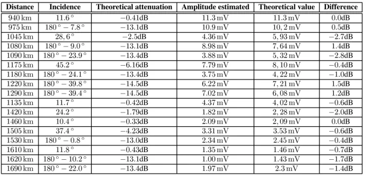
The magnitude of the current in the wire de"ned by (20) is theoretically very dependent on the incidence F of the wave, as it appears on "gure 6. Table 3 presents the comparison between the magnitude of the signal estimated for some records and their theoretical values computed from [9]. In the third column, the theoretical attenuations at (## *+, (2H&%# F'2 with % ! )-= ) are displayed illustrating variations of the antenna gain for some incidences. In the last column, the difference between the amplitudes estimated and their theoretical values are shown. It turns out that these differences are lower than )dB in practice. One may conclude that the radiation pattern produced by our model is close to reality.
8.2. Positioning accuracy.
Finally, the relevance of our model has been tested by the comparison of the propagation delay estimated with both models (!oating antenna and whip aerial). To achieve this goal, we had used several records with distances greater than those had used for identi"cation. The results are presented in table 4. It appears clearly that the whip aerial model is only relevant for incidences lower than 0# when our model is accurate for all incidences.
9. Conclusion.
We have presented a new way for modelling the behavior of the wire antenna used by submarines. The model leads to an important variation of the waveform when used with different incidence angles. It has been shown that the modelled waveforms match real data with a very good accuracy. Moreover, the variations of the antenna gain with the incidences are well treated by such a model.
0 10 20 30 40 50 60 -0.01 -0.008 -0.006 -0.004 -0.002 0 0.002 0.004 0.006 0.008 0.01 µs V Wire antenna Whip aerial Data
!gure 7: Comparison wire antenna / whip aerial - F ! (")
Consequently, it allows extending the use of transmitters with any azimuth, without change of course, as it is necessary at present time. Moreover, one can use at the same time several transmitting stations, which is known to improve the global location accuracy [10] [11].
Acknowledgements.
This work was supported by the DGA (General Army Direction - France) and the DIGINEXT company (France).
10. References.
[1] Ronold W. P. King, M Owens, and Tai Tsu Wu, Lateral Electromagnetic Waves - Theory and
Applications to Communications, Geophysical Exploration, and Remote Sensing, Springer-verlag,
1992.
[2] C Andréani-Corbabé, B Benhabiles-Lacour, M Depiesse, M Pellet, and C Pichot, “Etude
d’Antennes sous-marines pour la réception de signaux electromagnétique de très basse fréquence”, Annales des télécommunications, vol. 53, no. 7-8, pp. 835–850, 1998.
[3] Constantine A Balanis, “Antenna theory: A review”, Proceedings of the IEEE, vol. 80, no. 1, pp.
7–22, 1992.
[4] L Thourel, Antennes À Fil, vol. E3 280, Techniques de l’ingénieur.
[5] R W P King and G S Smith, Antennas in Matter: Fundamentals, Theory and Applications, The
MIT Press, Cambridge, MA, 1981.
0 10 20 30 40 50 60 -0.02 -0.015 -0.01 -0.005 0 0.005 0.01 0.015 0.02 µs V Wire antenna Whip aerial Data
!gure 8: Comparison wire antenna / whip aerial - F ! ()
[7] J D Last, R G Farnworth, and M D Searle, “Effect of skywave interference on the coverage of
LORAN-c”, IEE Proceedings, vol. 139, no. 4, pp. 306–314, 1992.
[8] Andrew H Jazwinski, Stochastic Processes and Filtering Theory, vol. 64, Academic press, New
York and London, 1970.
[9] “Groundwave propagation curves”, CCIR Rec. 368-5, vol. 5, 1986.
[10] A Monin, G Rigal, and P Charron, “A new technology for LORAN-c receivers”, in International
Symposium on Integration of LORAN-C/Euro!x and EGNOS/Galileo, Bonn, Germany, Mars
2000.
[11] A Monin and G Salut, “Optimal "ltering of LORAN-C signal via particle "ltering”, in EUSIPCO
Distance Incidence Theoretical attenuation Amplitude estimated Theoretical value Difference ,+$ -( !!%& #$%+!dB !!%" (. !!%" (. $%$dB ,)# -( !%$ # )%% #!"%!dB !$%, (. !$' ' (. $%#dB !$+# -( '%' & #'%#dB +%"& (. #' ," (. #'%)dB !$%$ -( !%$ # ,%$ #!"%!dB %%,% (. )' &+ (. !%+dB !$,$ -( !%$ # '"%, #!"%+dB "%%% (. #' "' (. #'%%dB !!)# -( +#%' #&%!&dB )%), (. %' !$ (. #$%+dB !!%$ -( !%$ # '+%! #!"%+dB "%)# (. +' '' (. #!%$dB !''$ -( !%$ # ",%% #!+%#dB &%'' (. )' '! (. !%#dB !',$ -( !%$ # ",%+ #!+%#dB )%$' (. &' $% (. !%'dB !!"# -( !!%) #$%+'dB +%") (. +' $' (. #$%&dB !+'$ -( '+%' #!%),dB !%%' (. '' '% (. #'%$dB !+&$ -( !$%+ #$%""dB '%$, (. '' $, (. $%$dB !#$# -( ")%+ #+%'"dB "%"! (. "%#" (. #$%&dB !#"$ -( !%$ # $%% #!"%$dB '%"+ (. '%+# (. #$%+dB !&!$ -( !!%% #$%+"dB !%"# (. !%+& (. #$%)dB !&'$ -( !%$ # !$%' #!"%!dB !%$$ (. !%+" (. #!%)dB !&,$ -( !%$ # ''%$ #!"%+dB !%,) (. '%" (. #!%+dB
table 3: Amplitudes estimated and their theoretical values.
Distance Incidence Floating antenna Whip aerial
,+$ -( !!' & #' ( #'" ( ,)# -( !%$ # )' % ! ( "%&" ( !!)# -( +#' ' #!! ( !+& ( !$+# -( '%' & #" ( &) ( !$%$ -( !%$ # ,' $ "" ( %,! ( !""# -( !!' ) #+# ( #&# ( !''$ -( !%$ # ",' % #'& ( &,# ( !',$ -( !%$ # ",' + #"& ( )&" ( !$,$ -( !%$ # '"' , #!! ( "%'$ ( !!%$ -( !%$ # '+' ! '% ( %', ( !+'$ -( '+' ' #%' ( #%& ( !+&$ -( !$' + % ( #') ( !#$# -( ")' + #!& ( #"" ( !#"$ -( !%$ # $' % #!% ( %!% ( !&!$ -( !!' % !# ( #!% ( !&,$ -( !%$ # ''' $ #+ ( ))# ( !&'$ -( !%$ # !$' ' #+# ( )&% (