Controlling Morphology and Resistivity in Multiphase Polymer Blends with Poly(ether-b-amide)

(1)

UNIVERSITÉ DE MONTRÉAL

CONTROLLING MORPHOLOGY AND RESISTIVITY IN MULTIPHASE POLYMER BLENDS WITH POLY(ETHER-B-AMIDE)

JUN WANG

DÉPARTEMENT DE GÉNIE CHIMIQUE ÉCOLE POLYTECHNIQUE DE MONTRÉAL

THÈSE PRÉSENTÉE EN VUE DE L’OBTENTION DU DIPLÔME DE PHILOSOPHIAE DOCTOR

(GÉNIE CHIMIQUE) MARS 2016

(2)

UNIVERSITÉ DE MONTRÉAL

ÉCOLE POLYTECHNIQUE DE MONTRÉAL

Cette thèse initulée:

CONTROLLING MORPHOLOGY AND RESISTIVITY IN MULTIPHASE POLYMER BLENDS WITH POLY(ETHER-B-AMIDE)

présentée par : WANG Jun

en vue de l’obtention du diplôme de : Philosophiae Doctor a été dûment acceptée par le jury d’examen constitué de :

M. TAVARES Jason-Robert, Ph. D., président

M. FAVIS Basil, Ph. D., membre et directeur de recherche Mme HEUZEY Marie-Claude, Ph. D., membre

(3)

DEDICATION

(4)

ACKNOWLEDGEMENTS

First of all, I would like to thank my research supervisor, Prof. Basil D. Favis, for his continuous support, guidance, and understanding both in work and in life. He is a supervisor who not only focuses on research but also helps me to develop in all aspects to become a qualified independent researcher. His door has always remained open whenever I have a question and whatever the question is. Working with him is one of the most important periods in my life.

I would like to thank the persons from our industrial collaborator Arkema: Dr. Alejandra Reyna-Valencia, Dr. Eric Gamache, Dr. Frederic Malet, Ms. Laure Berdin Sguerra, Dr. Richard Chaigneau, Dr. Damien Rauline, Dr. Yves Deyrail and Dr. Quentin Pineau. They helped me on many aspects of the project and their hospitality during my visit to Arkema is also acknowledged. I want to give my thanks to the current and previous members of our research group, Ebrahim, Ali, Vahid, Nima, Sepehr, Ata, Dr. Pierre Sarazin and Dr. Nick Virgilio, for their help and the useful discussions we had.

I would like to thank Prof. Pierre Carreau for teaching me the “well-known” Transport Phenomena course. It forced me to sit down and read a textbook again and again – something that I had not done for years.

Thanks to Prof. Daniel Therriault, Michael D. Buschmann and Frederic Sirois for giving me access to their lab facilities.

I also want to thank the current and previous technicians, research assistants and administrative staff in the Department of Chemical Engineering, in particular, Melina Hamdine, Guillaume Lessard, Claire Cerclé, Gino Robin, Martine Lamarche, Ricardo Villanueva Vazquez, Robert Delisle and Julie Tremblay, for their help during my PhD study. Thanks to Sylvie St-Amour from FPInnovations for her assistance on mercury intrusion porosimetry.

Finally and most importantly, I want to give my thanks to my families. I want to thank my parents and my two older sisters for having always been so supportive and allowing me to do whatever I want to; I owe them everything. I want to thank my little boy Bryan for the happiness he has brought to me. Thanks to my mother-in-law for helping us to take care of Bryan. Lastly, I want to give my special thanks to my lovely wife, Xiaoyan; for over ten years, she has always been there for me. I’m so lucky to have her accompany in my life.

(5)

RÉSUMÉ

Mélanger des polymères conducteurs avec des polymères conventionnels est une méthode efficace pour produire de nouveaux matériaux dotés de propriétés électriques spécifiques. Comparés à des mélanges binaires, des systèmes de mélanges de polymères ternaires et quaternaires doivent présenter un seuil de percolation bien plus bas si un des composants est encapsulé par d’autres phases continue/percolée, avec un effet plus marqué si localisé à une interface continue/percolée. Cependant, la majorité des travaux publiés s’est concentré à l’examen du cas où la phase conductrice est située au cœur du système en raison de tensions interfaciales intrinsèques élevées avec d’autres polymères. Assembler un composant polymère conducteur à une interface continue directement par l’intermédiaire de mélanges à l’état fondu a rarement été rapporté dans la littérature. Par ailleurs, des études sur le développement de la morphologie d’une phase intermédiaire partiellement ou complètement mouillée dans des systèmes ternaires et quaternaires sont encore très limitées.

Dans cette thèse, des mélanges de polymères destinés à des applications antistatiques avec un copolymère PEBA conducteur ionique (composé de blocs alternés PEO et PA) au sein de systèmes binaires, ternaires et quaternaires ont été étudiés.

Dans un premier temps, deux mélanges binaires, LDPE/PEBA et PS/PEBA, avec des tensions interfaciales considérablement distinctes ont été préparés. La tension interfaciale du système initial a été évaluée à 8.0 mN/m, et le développement de la morphologie du PEBA pour ce système suit une coalescence de deux gouttes observée typiquement au sein de systèmes de tension interfaciale élevée. Le second système possède, de façon inattendue, une tension interfaciale de 1.6 mN/m, vraisemblablement en raison de la présence de liaisons hydrogène-π entre le PS et le bloc PEO. Une miscibilité partielle entre le PS et le PEBA (bloc PEO) est aussi confirmée par le déplacement de Tg pour le PS dans les mélanges. Bien qu’une continuité plus élevée soit observée à des fractions volumiques plus faibles en PS/PEBA que en LDPE/PEBA, la résistivité surfacique du PS/PEBA est plus élevée que celle du LDPE/PEBA sur une large plage de compositions. Ce résultat a été attribué à la miscibilité partielle et/ou la constriction importante au sein de la morphologie d’instabilité capillaire gelée lorsque le PEBA est mélangé avec le PS, ce qui influence le transfert de charge au sein de la phase PEBA. Un modèle conceptuel du

(6)

transport de charge dans le copolymère PEBA a également été proposé basé sur le phénomène de migration des protons dans les domaines PEO.

Dans la seconde partie de ce travail, un polymère conducteur ionique (PEBA) a été directement assemblé à l’interface continue de deux autres polymères grâce au procédé de mélangeage à l’état fondu. Deux mélanges ternaires de LDPE/PEBA/PET et LDPE/PEBA/PVDF, ont été préparés démontrant respectivement un mouillage partiel et un mouillage complet. Une transition novatrice de morphologie de mouillage partiel à mouillage complet a été identifiée au sein du système LDPE/PEBA/PET. Une analyse thermodynamique indique que le LDPE/PEBA/PET est un système faiblement partiellement mouillé, et le phénomène de transition a été attribué à l’effet de coalescence dominant par rapport au démouillage avec une concentration en augmentation de PEBA. Dans le cas d’un système LDPE/PEBA/PVDF complètement mouillé, de fines couches intactes de PEBA (~ 100 nm) ont été observées pour des concentrations de PEBA aussi faibles que 3%. Il apparaît clairement qu’une concentration minimale est requise afin de former une interface mouillée, et que cette concentration dépend de la valeur du coefficient d’étalement. L’auto-assemblage de PEBA à l’interface continue réduit considérablement le seuil de percolation dans des mélanges ternaires par rapport à des mélanges binaires. Dans le cas d’application antistatiques requérant une résistivité surfacique plus faible que 1013 Ω/sq, 20% de PEBA est nécessaire dans des mélange binaires conventionnels ; cette valeur se réduit à 10% pour les mélanges ternaires LDPE/PEBA/PET, et jusqu’à 1% pour le système LDPE/PEBA/PVDF.

La troisième partie de ce projet se consacre au contrôle de la localisation du PEBA dans des mélanges de polymères polyphasés à structure hiérarchisée. Il a été montré que lorsque des polymères conducteurs sont mélangés avec des polyoléfines et/ou du PS dans des mélanges ternaires, ils ont tendance à être situés au cœur en raison des tensions interfaciales élevées avec ces polymères. Néanmoins, mélanger des polymères conducteurs avec des polymères de grande consommation tels que les polyoléfines et le PS peut présenter des gains de coûts conséquents. Pour cette raison, un mélange ternaire de LDPE/PS/PEBA avec PEBA comme phase cœur a été choisi comme premier cas d’étude de cette partie du travail. Afin de contrôler la localisation du PEBA au sein de systèmes multiphasiques possédant une concentration élevée en LDPE/PS (70– 90%), un quatrième composant ou un modificateur interfacial a été ajouté. Dans les deux cas, le PEBA a été localisé avec succès sur une interface continue, et a formé des structures percolatées

(7)

dans les systèmes ternaires et quaternaires hiérarchiquement ordonnés. Ceci a permis une réduction significative de la résistivité surfacique d’un facteur de l’ordre de 2 à 4 en comparaison avec les mélanges ternaires initiaux de LDPE/PS/PEBA où le PEBA était situé au cœur.

Finalement, comme présenté dans l’annexe, afin de démontrer une approche généralisée aux structures hiérarchiques dans les mélanges ternaires, une nouvelle stratégie a été développée permettant de générer des polymères hiérarchiquement poreux où la taille des pores est contrôlée grâce à un système de mélange ternaire A/B/C-B-C.

(8)

ABSTRACT

Blending conductive polymers with conventional polymers has been an effective approach to produce new materials with tailored electrical properties. Compared to binary blends, ternary and quaternary polymer blend systems are expected to have a much lower percolation threshold if a component is encapsulated by other continuous/percolated phases, with a more dramatic influence when it is located at a continuous/percolated interface. However, almost all the published work has examined the case where the conductive phase is situated in the core of the system owing to its inherent high interfacial tensions with other polymers. Assembling a conductive polymeric component at a continuous interface directly through melt blending has rarely been reported. Also, studies on the morphology development of a partially wet or completely wet intermediate phase in ternary and quaternary systems are still very limited. In this dissertation, polymer blends destined for antistatic applications with an ionically conductive PEBA copolymer (comprised of alternating PEO and PA blocks) in binary, ternary and quaternary systems were studied. In the first part, two binary blends, LDPE/PEBA and PS/PEBA, with significantly different interfacial tensions were prepared. The interfacial tension for the former system was determined to be 8.0 mN/m and the morphology development for PEBA in this system follows a droplet-droplet coalescence mechanism typically observed in high interfacial tension systems. The latter system possesses, unexpectedly, a much lower interfacial tension of 1.6 mN/m, possibly owing to the presence of π-hydrogen bonding between PS and the PEO block. Partial miscibility between PS and PEBA (the PEO block) is also confirmed by the shift of Tg for PS in the blends. Although a higher continuity is observed at lower volume fractions in PS/PEBA than in LDPE/PEBA, the surface resistivity for PS/PEBA is surprisingly higher than that of LDPE/PEBA over a wide range of compositions. This result was attributed to the partial miscibility and/or the significant constriction in the frozen capillary instability morphology when PEBA is blended with PS, which influences the charge transfer in the PEBA phase. A conceptual model for charge transport in the PEBA copolymer based on the migration of protons in the PEO domains is also proposed.

In the second part of this work, we assembled an ionically conductive polymer (PEBA) at the continuous interface of two other polymers directly through melt blending. Two ternary blends of LDPE/PEBA/PET and LDPE/PEBA/PVDF were prepared which demonstrate partial wetting and

(9)

complete wetting respectively. A novel morphology transition from partial wetting to complete wetting was identified in the LDPE/PEBA/PET system. Thermodynamic analysis indicates that LDPE/PEBA/PET is a weak partial wetting system and the transition phenomenon was attributed to the dominant effect of coalescence over dewetting with increasing PEBA concentration. In the case of the completely wet LDPE/PEBA/PVDF system, thin intact PEBA layers (~ 100 nm) were observed at PEBA concentrations as low as 3%. It appears clear that a minimum concentration is required to form a completely wet interface and that this concentration depends on the value of the spreading coefficient. The self-assembling of PEBA at the continuous interface dramatically reduces its percolation threshold in the ternary blends as compared to binary blends. For antistatic applications requiring a surface resistivity lower than 1013 Ω/sq, 20% of PEBA is needed in the conventional binary blends; the value is reduced to 10% for LDPE/PEBA/PET, and to as low as 1% for the LDPE/PEBA/PVDF system. The third part of the project focuses on controlling the localization of PEBA in hierarchically ordered multiphase polymer blends. It has been shown that when conductive polymers are blended with polyolefins and/or PS in ternary blends, they tend to be located in the core due to its high interfacial tensions with these polymers. Nevertheless, blending conductive polymers with commodity polymers such as polyolefins and PS can present significant potential cost advantages. Thus, we started this part of the work with a ternary blend of LDPE/PS/PEBA where PEBA is the core phase. In order to control the localization of PEBA in the multiphase systems with high LDPE/PS content (70–90%), either a fourth component or an interfacial modifier was added. In both cases, PEBA was successfully localized to a continuous interface and formed percolated structures in the hierarchically ordered ternary and quaternary systems. This led to a significant reduction of 2–4 orders of magnitude in surface resistivity as compared to the initial ternary blends of LDPE/PS/PEBA where PEBA was located in the core. Finally, as shown in the Appendix, in order to demonstrate a generalized approach to hierarchical structures in ternary blends, we developed a new strategy to generate hierarchically porous polymers with controllable pore size through a ternary A/B/C-B-C blend system. PLA/HDPE/SEBS was used as a model system.

(10)

LIST OF TABLES

Table 2.1: Commercially available PEBA copolymers and their composition (taken from Ref.

[55]). ... 14

Table 4.1: Characteristics of the materials used ... 45

Table 4.2: Interfacial tension between different polymers ... 51

Table 4.3: Structural parameters for the PEBA copolymer ... 53

Table 5.1: Characteristics of the polymers used ... 79

Table 5.2: Interfacial tensions, spreading coefficients and predicted morphologies (PEBA is the minor phase) ... 83

Table 5.3: The distribution of PEBA and the interfacial area in the ternary blends ... 88

Table 6.1: Characteristics of the materials used* ... 110

Table 6.2: Interfacial tension and spreading coefficient for LDPE/PS/PEBA (200°C) ... 115

Table 6.3: Interfacial tensions and spreading coefficients in LDPE/PS/PEBA/PET (250°C) and LDPE/PS/PEBA/PVDF (200°C)* ... 116

Table 6.4: Interfacial tensions and spreading coefficients of the EAM modified LDPE/PS/PEBA (200°C) ... 124

Table 7.1: Different wetting behaviours at different interfaces in the ternary PE/PP/PS blend .. 139

Table A1: Interfacial tensions between different polymers at 200°C (PE/SEBS at 195°C) ... 159

(16)

LIST OF FIGURES

Figure 1.1: Examples of advanced structures developed in multi-phase polymer blends. a) tri-continuous structures in PE/PS/PMMA ternary blends (PMMA extracted) (taken from Ref. [10]); b) PS forms completely wet layer at the interface of HDPE/PMMA with a high continuity (about 70%) achieved at 3% (taken from Ref. [11]); c) PS self-assembles into close-packed droplet array at the PE/PP interface (taken from Ref. [28]); d-e) tune the morphology of PS at the interface of PA/PC from partially wet droplets to completely wet layers by adding PS-g-MA (taken from Ref. [13]); f) confine CNTs within thin EMAA layers formed at the PP/PA interface to reduce the percolation threshold (taken from Ref. [23]). ... 3 Figure 2.1: Development of conductive pathways in polymer composite systems as a function of

filler concentration (taken from Ref. [34]). ... 4 Figure 2.2: Structures and conductivities of some conjugated conductive polymers (taken from

Ref. [33]). ... 6 Figure 2.3: Schematic of conductive mechanism in polyactylene with an oxidative dopant (taken

from Ref. [37]). ... 6 Figure 2.4: Ion transport in PEO: a) Lateral migration of the cation through C-O bond rotation

along the AB line; b) the transfer of the cation between PEO chain segments by oxygen ligand replacement (taken from Ref. [32]). ... 7 Figure 2.5: Schematic for the measurement of the surface resistivity. U and I are the applied

voltage and measured current; g, D0, D1 and D2 are the geometry parameters of the

measuring setup. ... 9 Figure 2.6: Charge dissipation mechanism of migrating antistats (adapted from Ref. [1]). ... 11 Figure 2.7: Schematic of dissipative networks developed in the IDP/host polymer binary blend

(taken from Ref. [1]). ... 12 Figure 2.8: Schematic of the general chemical structure of a PEBA copolymer (adapted from

(17)

Figure 2.9: Synthesis of ester-linked PEBA copolymers through the two-step thermal polymerization (taken from Ref. [55]). ... 15 Figure 2.10: a) Schematic representation of PEBA solid-state structures; b) TEM image of a

poly(ether-b-amide) copolymer with a polyamide/polyether weight ratio of 23/77 (taken from Ref. [5, 55]). ... 15 Figure 2.11: Theoretical morphology factor fideal of polyelectrolytes with different morphologies.

The blue region represents the conducting phase (taken from Ref. [62]). ... 17 Figure 2.12: Schematic representation of ion transport in the PS-PEO-PS electrolytes (taken from

Ref. [45]). ... 18 Figure 2.13: Electrostatic dissipation mechanism via hydrogen-bondings between PEO/water and

amide/water. The partial ionization of water molecules generates protons for charge dissipation (taken from Ref. [8]). ... 19 Figure 2.14: Three typical states of miscibility in a binary system: (A) completely immiscible;

(B) completely miscible; and (C) partially miscible (taken from Ref. [67]). ... 20 Figure 2.15: Schematic presentation of morphology development in binary polymer blends (taken

from Ref. [10]). ... 21 Figure 2.16: Schematic representation of flow-induced coalescence of two droplets in a

Newtonian system. The two droplets are brought close to each other and rotate in the flow filed; the film in-between thins and finally raptures; the two droplets contact and emerge into one (taken from Ref. [77]). ... 23 Figure 2.17: Mechanism for morphology development in systems of low interfacial tension (a)

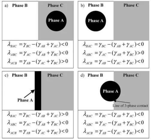
and high interfacial tension (b) (taken from Ref.[74]). ... 24 Figure 2.18: Possible morphologies in a ternary blend of A/B/C as predicted by Harkins’

spreading theory (A is the minor phase). (a)-(c): complete wetting, one phase fully separate the rest two; (d) partial wetting, three phase contact (taken from [28]). ... 26 Figure 2.19: Three-dimensional schematic representation of the multiple percolated structures in

the ternary HDPE/PS/PMMA system: thin PS layer is at the HDPE/PMMA interface (taken from Ref. [11]). ... 27

(18)

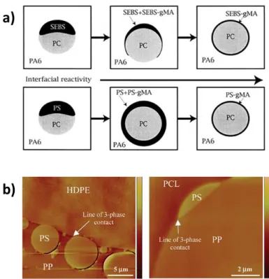
Figure 2.20: (a) Different morphology evolution patterns in PA6/SEBS/PC and PA6/PS/PC after adding SEBS-MA and PS-MA respectively (which gradually replace SEBS and PS in the two systems) as interfacial modifiers (taken from Ref. [13]). (b) Morphologies of the annealed HDPE/PS/PP and PP/PS/PCL blends (taken from Ref. [93]). PS droplets appear more spherical in the former and more extended along the PP/PCL interface in the latter. .. 28 Figure 2.21: (a) Four sets of spreading coefficients of the quaternary HDPE/PP/PS/PMMA blend.

(b) AFM image of the HDPE/PP/PS/PMMA (45/45/5/5) blend after 30 min of annealing; the lines of three phase contact for HDPE/PS/PP and PP/PS/PMMA are indicated by arrows (taken from Ref. [94]). (c) TEM image of PBT/PS/SAN/PC (taken from Ref. [89]). ... 29 Figure 2.22: Three possible morphologies of a ternary system with a matrix A and two dispersed

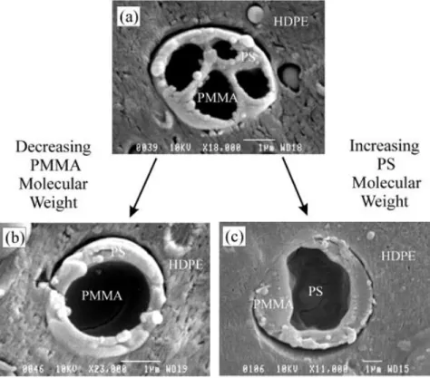
phases B and C (taken from Ref. [95]). B+C: phase B and phase C are separated by the matrix A; B/C: phase C is encapsulated by phase B in the matrix A; C/B: phase B is encapsulated by phase C in the matrix A. ... 31 Figure 2.23: Effect of molecular weight on the morphology in ternary HDPE/PS/PMMA blends.

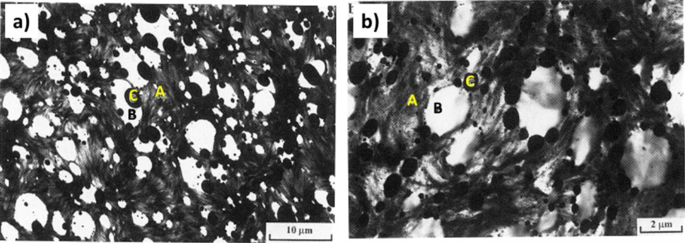
(a) and (b): PMMA is encapsulated by PS (PMMA was extracted); (c) PS is engulfed by PMMA (PS was extracted) (taken from Ref. [91]). ... 32 Figure 2.24: Morphology of the ternary blend of HDPE/PP/PS (70/20/10): (a) without SEB; (b)

with 1% SEB. Polymer phases: A–HDPE, B–PP, and C–PS (taken from Ref. [95]). ... 33 Figure 2.25: The localization of solid particles in polymer blends predicted by Young’s Equation.

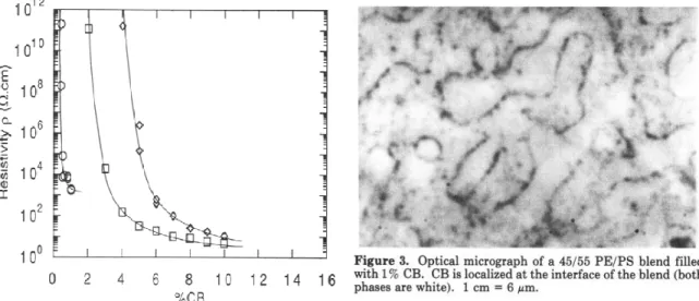
(a): within Phase 2 when 𝜔 > 1; (b) at the interface when -1 < 𝜔 < 1; (c) within Phase 1 when 𝜔 < -1 (taken from Ref. [106]). ... 35 Figure 2.26: Effect of selective localization on the resistivity in the PE/PS/CB (45/55/X) blends

as compared to the PE/CB blends (left image): PE/CB (◊); CB in PE phase in the PE/PS/CB system (□); CB at the interface of the PE/PS in PE/PS/CB system (○). Optical micrograph of PE/PS/CB (45/55/1) where CB is confined at the PE/PS interface (right image) (taken from Ref. [18]). ... 36 Figure 2.27: Schematic representation of confining CNT at the interface by a completely wet

(19)

highest affinity with the B phase among the three components in the ternary blend (taken from [22]) ... 37 Figure 4.1: (a) Complex viscosity and (b) storage modulus (filled symbols)/loss modulus (open

symbols) of the raw materials. ... 50 Figure 4.2: SAXS intensity as a function of the magnitude of the scattering vector q. The two

arrows indicate the two peaks detected. ... 52 Figure 4.3: (a) The glass transition temperatures of PS and PEBA in the PS/PEBA blends; (b)

crystallization behaviour of PEBA, PS and the PS/PEB blends during cooling. Dashed line indicates Tg of PS ... 56 Figure 4.4: Continuity of PEBA in LDPE/PEBA and PS/PEBA blends. ... 58 Figure 4.5: Morphology of the LDPE/PEBA and PS/PEBA blends with different volume

fractions. LDPE/PEBA: (a) 90/10; (b) 80/20; (c) 70/30. PS/PEBA: (d) 90/10; (e) 80/20; (f) 70/30. PEBA was extracted. Circles indicate signs of connections between the PEBA domains. ... 59 Figure 4.6: Morphology of the PEBA phase in the PS/PEBA and LDPE/PEBA blends with

different compositions after LDPE and PS are selectively dissolved. ... 61 Figure 4.7: PEBA phase size in different blends obtained from IA (PEBA volume fraction  20%)

and MIP (PEBA volume fraction > 20%). The dashed line for LDPE/PEBA system indicates the approximate concentration limit for droplets (left side) and fibers (right side). For PS/PEBA the phase size indicates a fiber diameter at all concentrations. ... 62 Figure 4.8: Schematic illustration of continuity development by frozen capillary instability in

PS/PEBA up to 10% concentration. ... 63 Figure 4.9: Surface resistivity in the LDPE/PEBA and PS/PEBA blends as a function of PEBA

composition. The horizontal dashed line indicate the surface resistivity of pure PEBA. ... 65 Figure 4.10: Effect of water content on surface resistivity for pure PEBA and its binary blends

with LDPE and PS. ... 66 Figure 4.11: Schematic representation of the charge dissipation mechanism in the PEBA binary

(20)

Figure 5.1: Partial and complete wetting morphologies in ternary blends of A/B/C predicted by Harkins’ spreading theory (B: the minor phase at interface) ... 77 Figure 5.2: Complex viscosities of the neat polymers at 200 and 250°C. The dashed line indicates

the processing shear rate of 25 s-1. ... 82 Figure 5.3: SEM images of cryo-microtomed LDPE/PEBA/PET blends with increasing PEBA

composition. The right column shows the effect of phosphotungstic acid staining at a higher magnification (the white phase is PEBA). Photo (d) presents the observed two typical morphologies (layer and droplets) in different spots as separated by the line. ... 85 Figure 5.4: SEM images of cryo-fractured LDPE/PEBA/PET blends (the white domains are

PEBA stained by phosphotungstic acid) ... 86 Figure 5.5: SEM images of cryo-fractured LDPE/PEBA/PVDF blends at different PEBA

compositions (the white domains are PEBA stained by phosphotungstic acid). ... 87 Figure 5.6: Domain thickness of PEBA at the interface in the ternary blends. Filled symbols:

measured directly from SEM images; open symbols: calculated based on the amount of PEBA at the interface and the interfacial area. ... 89 Figure 5.7: Surface resistivity of the binary and ternary blends. The dashed lines indicate the

boundary of the two stages (steep reduction and gradual reduction) and the dotted line shows the surface resistivity of neat PEBA. ... 91 Figure 5.8: Morphology of the blends (PEBA is stained by phosphotungstic acid) after annealing

for 10 min. (a) and (b): LDPE/PEBA/PET 50/3/47 and 50/10/40 at 260°C; (c) and (d): LDPE/PEBA/PVDF 50/3/47 and 50/10/40 at 200°C. Scale bar: 10 µm... 93 Figure 5.9: Schematic of the Neumann triangle: the equilibrium profile of a liquid B situated at

the interface of liquids A and C. ... 94 Figure 5.10: Schematic of the transition from partial wetting to complete wetting in weak partial

wetting systems (Plane direction: perpendicular to the interface for top images and along the interface for lower images). ... 95 Figure 5.11: Morphology of cryo-fractured LDPE/PEBA/PET (50/35/15) annealed at 250°C for

(21)

Figure 5.12: An example of an LDPE/PEBA/PET cryo-fractured sample for interface coverage calculation ... 103 Figure 5.13: Interface coverage by PEBA at the LDPE/PET interface in LDPE/PEBA/PET blends ... 103 Figure 5.14: Volume resistivity of the blends. ... 103 Figure 5.15: Geometrical parameters of the LDPE/PEBA/PET (50/3/47) blend for determining

the Neumann angle θ. ... 104 Figure 6.1: Possible morphologies in ternary blends of A/B/C predicted by Harkins’ spreading

theory (C is the minor phase). ... 108 Figure 6.2: Morphology of LDPE/PS/PEBA with a volume fraction of 75/20/5 (PEBA extracted). ... 113 Figure 6.3: Morphology evolution in LDPE/PS/PEBA (50/X/Y) as the volume fraction of PEBA

increases. Scale bar: 10 µm. ... 114 Figure 6.4: Morphology of the quaternary blends of LDPE/PS/PEBA/PET at different

compositions (the white phase is PEBA stained by phosphotungstic acid). Cryo-microtomed samples: (a) 50/20/10/20 and (b) 50/22.5/5/22.5; cryo-fractured samples: (c) 50/22.5/5/22.5 and (d) 50/23.5/3/23.5. ... 118 Figure 6.5: Morphology of the LDPE/PS/PEBA/PET quaternary blends at different compositions

(the white phase is PEBA stained by phosphotungstic acid). Cryo-microtomed samples: (a) 50/20/10/20; cryo-fractured samples: (b) 50/20/10/20; (c) 50/22.5/5/22.5 and (d) 50/23.5/3/23.5. ... 119 Figure 6.6: Surface resistivity of the binary, ternary blends and quaternary blends with PEBA.

The horizontal dashed line shows the surface resistivity of pure PEBA. ... 121 Figure 6.7: Schmatics of morphology and surface resistivity evolution in LDPE/PEBA,

LDPE/PS/PEBA, LDPE/PS/PEBA/PET and LDPE/PS/PEBA/PVDF. ... 122 Figure 6.8: Morphology of the ternary LDPE/PS/PEBA (50/40/10) blends (microtomed surface

(22)

and (b) 30 min. Modified with EAM and annealed at 200°C for (c) 0 min, (d) 10 min and (e) 30 min. Scale bar: 10 µm. ... 125 Figure 6.9: Surface resistivity of LDPE/PS/PEBA 50/40/10 with and without modification by

EAM after annealing at 200°C for different periods of time. ... 127 Figure 6.10: Detailed morphology of LDPE/PS/PEBA (50/40/10) with EAM after 30 min of

annealing at 200°C (the white phase is PEBA which is stained by phosphotungstic acid). (a) and (b) are cryo-microtomed samples; (c)–(f) are cryo-fractured samples at different magnifications. ... 128 Figure 6.11: Schematic comparison of the morphology after annealing between the PE/PP/PS

(modified with SEB) system from previous work (a) 19 and the PE/PS/PEBA (modified with EAM) system in this study (b). ... 129 Figure 6.12: Morphology of the quaternary LDPE/PS/PEBA/PET blends with different

formations characterized by SEM (the white phase is PEBA which is stained by phosphotungstic acid). (a) and (b): LDPE/PS/PEBA/PET (50/10/10/30) at low and high magnifications; (c): LDPE/PS/PEBA/PET (50/20/10/20); (d) LDPE/PS/PEBA/PET (50/30/10/10). ... 136 Figure 6.13: The proportions of PEBA in PS, PET and at the interface of PS/PET in the

quaternary LDPE/PS/PEBA/PET blends (the small amount of PEBA in LDPE is neglected). ... 137 Figure 7.1: Two scenarios of effect of interfacial modification on phase localization in ternary

polymer blends (Phase 3: the minor component). Case (a): change from partial wetting to complete wetting, has already demonstrated in literature. Case (b): change from complete wetting to another complete wetting, has not been reported. ... 140 Figure A1: Complex viscosity and elastic modulus as a function of angular frequency at 200°C. ... 160 Figure A2: SEM and MIP results: a) ~ c): PLA/HDPE/SEBS (50/45/5, 50/35/15, 50/25/25, SEBS

extracted by cyclohexane); d) PLA/HDPE/SEBS (50/25/25, PLA and SEBS extracted by chloroform); e) PLA/HDPE (50/50, PLA extracted by chloroform); f) HDPE/SEBS (50/50, SEBS extracted by cyclohexane); g) Mercury Intrusion Porosimetry (MIP) results. ... 163

(23)

Figure A3: AFM phase images: a, b, c) HDPE/PLA/SEBS (25/50/25) at different magnifications; d) pure SEBS; e) HDPE/SEBS (50/50); f) PLA/SEBS (50/50). Scale bar: 1μm. ... 165 Figure A4: Pore size evolution for the ternary blend (PLA/HDPE/SEBS 50/25/25) annealed at

200°C for a period of 60 min (data obtained after extracting PLA and SEBS from the blends). ... 167 Figure A5: Morphology of the annealed (at 220°C for 60 min) ternary blends PLA/HDPE/SEBS

with volume fractions: a) 50/25/25, b) 50/40/10, and c) 60/32/8. ... 169 Figure A6: Pore size distribution (MIP results) of the blends PLA/HDPE/SEBS with different

volume fractions after anealed at 220°C for 60 min ( the smaller pore size region is further shown in the inserted image). ... 169 Figure A7: Time sweep measurements performed at 0.1 Hz ... 173 Figure A8: Morphology evolution of PLA/HDPE/SEBS 50/25/25 during annealing at 200°C

(24)

LIST OF SYMBOLS AND ABBREVIATIONS

English Letters:

a molecular length

A area

e film thickness

G Gibbs free energy

H enthalpy

k numerical dissipation factor

m weight n number of moles P perimeter q scattering vector R radius S entropy Ca capillary number

Tg glass transition temperature

Tm melting temperature

Mn number average molecular weight Mw weight average molecular weight

Greek Letters:

α0 initial distortion amplitude

β constriction factor

 volume fraction

(25)

𝛾̇ shear rate σ conductivity γ interfacial tension τ shear stress/tortuosity ω wetting parameter λ spreading coeffcient

θ Neumann angle (contact angle)

µ chemical potential

v dewetting speed

List of Abbreviations:

ABS acrylonitrile-butadiene-styrene copolymer AFM atomic force microscope

CB carbon black

CNT carbon nanotubes

EAM ethylene–acrylic ester–maleic anhydride random terpolymer EMAA poly(ethylene-co-methacrylic acid)

ESD electrostatic discharge HDPE high-density polyethylene ICP inherently conductive polymer IDP inherently dissipative polymer LDPE low-density polyethylene

MA maleic anhydride

PA polyamide

(26)

PBT polybutylene terephthalate

PC polycarbonate

PE polyethylene

PEBA Poly(ether-b-amide) PEO poly(ethylene oxide) PET polyethylene terephthalate PMMA poly(methyl methacrylate)

PP polypropylene

PPO poly(propylene oxide)

PTCNQ poly(tetracyanoquinodimethane) PTMO poly(tetramethylene oxide) PPV polyparaphenylene vinylene PPY polypyrrole PS polystyrene PT polythiophene PTTF poly(tetrathiafulvalene) PVDF polyvinylidene fluoride PVF(c) poly(vinylferrocene)

SAXS small angle X-ray scattering SAN poly(styrene-co-acrylonitrile)

SEBS styrene-ethylene/butylene-styrene triblock copolymer SEB styrene-(ethylene-butylene) diblock copolymer SEM scanning electron microscope

(27)

LIST OF APPENDICES

APPENDIX ARTICLE 4: HIERARCHICALLY POROUS POLYMERIC MATERIALS FROM TERNARY POLYMER BLENDS………...155

(28)

CHAPTER 1 INTRODUCTION

More than two thousand years ago, the Greek scientist Thales of Miletus discovered that amber attracts small dust particles when rubbed with animal fur – a phenomenon of static electricity. In modern society, static electricity has emerged as a common problem in many areas associated with the usage of polymeric materials which themselves are electrical insulators in most cases. Electrical charge accumulation and uncontrolled electrostatic discharge (ESD) on a polymer surface can cause issues such as dust adsorption, damage to electronic components and even initiating explosion, which are encountered in many industrial sectors, including electronics, medicine and pharmacy, automotive, aerospace, mining, etc. [1-3]. To avoid static charge accumulation while maintaining the nonconductive nature, the surface resistivity of the polymeric parts generally needs to be reduced to the range of 109–1013 Ω/sq (technically termed as antistatic materials). However, most conventional polymers fail to meet this criterion.

Many additives have been developed and added to conventional polymers to tailor the surface resistivity according to different applications. Among them, conductive polymers are particularly effective in providing long-term and reliable ESD protection, and they also bear the colorable and non-sloughing features which are desired for many applications [1, 4]. After blending with the host polymers (e.g., PE, PP, PET, PS, etc.), conductive polymers can develop three-dimensional conductive pathways throughout the blend for charge dissipation. Ionically conductive poly(ether-b-amide) (PEBA) copolymers take a major share in this antistat category and the commercial products include Arkema Pebax®, BASF Irgastat® P and Sanyo Pelestat®. These copolymers also display very good processibility, thermal stability and mechanical properties [5]. The final product with PEBA for antistatic applications is typically a binary polymer system (comprised of a host polymer and a conductive polymer) requiring high composition (10–25%) for the polymeric antistat to develop electrical percolation in the host polymer, which increases the cost and may also deteriorate certain physical properties (e.g., mechanical performance, clarity, etc.). Meanwhile, despite the commercial success for PEBA, very limited work has been published to study the effect of PEBA continuity/morphology on surface resistivity of the blends, particularly in multiphase systems [6, 7]. Furthermore, the studies on the charge dissipation mechanism in these copolymers are also very limited [8, 9].

(29)

The study of morphology in multiphase polymer blends has been attracting increasing attention over the past 15 years [10-14]. Different from the binary blends where dispersed phase/matrix and co-continuous morphologies are observed, complex structures can be obtained in multiphase polymer systems (Fig. 1.1). The multi-percolated structures generated from multiphase polymer blends are of particular interest in terms of reducing the percolation threshold of PEBA and achieving the required surface resistivity for antistatic applications at low PEBA compositions. Previous studies with other conductive polymers have shown that much higher conductivity can be obtained in these systems as compared to in traditional binary blends [15-17]. However, in almost all the work published on the melt processing of conductive polymer blends, the conductive component is situated in the core and encapsulated by other polymers (rather than at the interface) [6, 15-17]. In this context, the well documented studies on conductive composites demonstrate the significant advantage of placing the conductive inorganic fillers (e.g., carbon black, carbon nanotube, etc.) at the interface for improved electrical conductivity [18-23]. These results point to the great potential to significantly lower the electrical percolation threshold by confining PEBA at the interface of the host polymers. In practice, it is desirable to obtain the structures through melt blending since it is a cost-effective technique widely used in industry. In ternary polymer blends with two major phases A and C and a minor phase B located at the interface of A/C, the phase B can adapt to either layer (B completely wets the A/C interface; e.g., Fig. 1.1b: PS layer at HDPE/PMMA interface) or droplet (B partially wets the A/C interface; e.g., PS droplets at the PE/PP interface as shown in Fig. 1.1c) morphology depending on the spreading coefficients [24, 25]. The former scenario has attracted much research effort due to its ability to develop percolation at very low concentrations [11, 23, 26, 27]. However, some important questions, for example, whether there exists a minimum layer thickness to achieve full segregation and what factors may control this thickness, have been barely investigated [27]. In the latter scenario, some studies indicate the droplets are discrete at the interface [28, 29]. Other studies reported on the transformation from partial wetting to complete wetting by adding an interfacial modifier (Figs. 1.1d and e) [12, 13]. To date, it is still not clear how the morphology of the intermediate phase evolves during processing. Understanding these questions will benefit the advanced applications of these complex but well-controllable structures.

(30)

Figure 1.1: Examples of advanced structures developed in multi-phase polymer blends. a) tri-continuous structures in PE/PS/PMMA ternary blends (PMMA extracted) (taken from Ref. [10]); b) PS forms completely wet layer at the interface of HDPE/PMMA with a high continuity (about 70%) achieved at 3% (taken from Ref. [11]); c) PS self-assembles into close-packed droplet array at the PE/PP interface (taken from Ref. [28]); d-e) tune the morphology of PS at the interface of PA/PC from partially wet droplets to completely wet layers by adding PS-g-MA (taken from Ref. [13]); f) confine CNTs within thin EMAA layers formed at the PP/PA interface to reduce the percolation threshold (taken from Ref. [23]).

a b d e f PA PC PS+ PS-g-MA PS c PE PS

(31)

CHAPTER 2 LITERATURE REVIEW AND OBJECTIVES

2.1 Conductive Polymer Systems

According to the range of electrical conductivity, solid materials can be divided into three groups: conductors, semiconductors and insulators [30]. Although polymers are traditionally used as insulators, conductive polymer systems have also been developed which can be classified into four types: 1) conductive polymer composites; 2) conjugated polymers; 3) ionically conductive polymers; and 4) redox polymers. The electrical conductivity in these systems can arise from the flow of electrons (electronically conductive polymers) and/or from the net motion of charged ions (ionically conductive polymers) [31, 32].

2.1.1 Conductive Polymer Composites

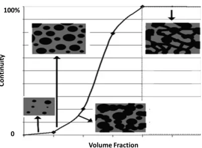
The most widely used conductive polymers are polymer composites where electrical conductivity is imparted by adding conductive fillers (such as carbon and metal particles) to the insulating polymer matrix [33]. Generally, the development of conductive pathways in these systems can be divided into three regions as a function of filler content (Fig. 2.1). At low filler loading, the fillers remain discrete and the conductivity of the composite shows little improvement as compared to the pure polymer (region A). After exceeding a critical point (percolation threshold), the conductive network develops through filler contact and the conductivity increases steeply (region B). Further increasing the filler amount leads to a slight monotonic increment approaching the intrinsic conductivity of the filler (region C).

Figure 2.1: Development of conductive pathways in polymer composite systems as a function of filler concentration (taken from Ref. [34]).

(32)

2.1.2 Conjugated Polymers

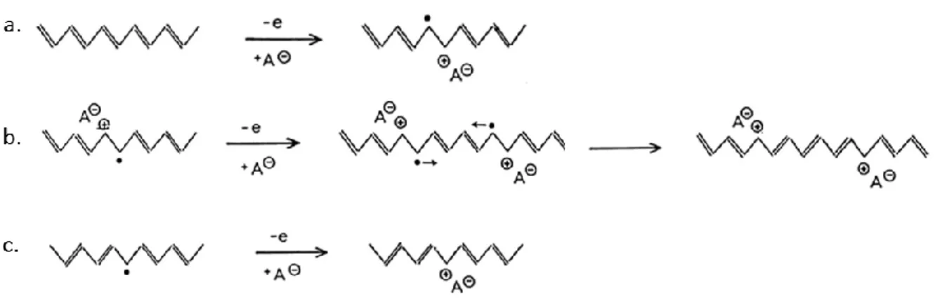
Conjugated polymers are characterized by alternating single and double bonds which results in an extended π electron system. The interest in conjugated conductive polymers started in the 1970s when the conductivity of polyacetylene films was dramatically improved after it was exposed to iodine vapor [35, 36]. Following this work, a variety of conjugated polymers have been synthesized, including, polypyrrole (PPY), polythiophene (PT), polyaniline (PANI), polyparaphenylene vinylene (PPV), etc. Fig. 2.2 shows the structures of some of the conjugated conductive polymers and their conductivities. These polymers are inherently conducting due to the conjugated π electron system and thus are also referred to as inherently conductive polymers (ICPs). However, their original conductivities are very low (e.g., polyacetylene from cis-isomers has a conductivity of 10-9 S/cm at 273K [35]), but can be increased by oxidation (p-doping) and/or, reduction (n-doping) to generate mobile charge carriers. For example, in the well-known work on polyacetylene from Shirakawa, MacDiarmid and Heeger, the conductivity of polyacetylene (from trans-isomers) was increased from 3.3×10-6 to 30 S/cm by iodine doping [35]. The mechanism of this process is briefly presented in Fig. 2.3 by using oxidation as an example [37]. After doping, an electron is removed from the π system which leads to the delocalization of a radical ion (polaron) as shown in Fig. 2.3a. Further oxidation and radical recombination yields two charged carriers on the chain (Fig. 2.3b). Meanwhile, a number of neutral defects also exist in the synthesized polyacetylene (solitons) and charged soltions can be generated after oxidation (Fig. 2.3b). These delocalized charges are mobile (but not the dopant ions) along the polymer chain and also capable of traveling to other chains through hopping which make current conduction through the bulk possible. Due to the intrinsic conjugated structures on the backbone, unfunctionalized conjugated polymers are usually insoluble, infusible and brittle, which limit their wide applications [32].

(33)

Figure 2.2: Structures and conductivities of some conjugated conductive polymers (taken from Ref. [33]).

Figure 2.3: Schematic of conductive mechanism in polyactylene with an oxidative dopant (taken from Ref. [37]).

2.1.3 Ionically Conductive Polymers

Ionic conductivity is generally restricted to salt solutions (with polar solvent) or molten salts. The ion transportation in solid polymers without a solvent was only recognized a few decades ago in the 1970–80s [38-41]. The macromolecule acts as a solvent to partially disassociate the salt, resulting in a complex system with electrolyte behaviour. Thus, ionically conductive polymers are also known as polymer electrolytes [31, 32, 41]. It is generally accepted that the conductivity originates from ion migration between coordination sites generated by the local segmental motion of the polymer chains [31, 42-44] (Fig. 2.4). Therefore, ionically conductive polymers are expected to bear electron-donating atoms or groups to coordinate with cations and low bond rotation barriers (flexible bonds and weak inter-chain interactions) to facilitate segmental motion

(34)

[32]. Poly(ethylene oxide) (PEO) (as well as its copolymers) remains the most extensively studied ionically conductive polymer, particularly as solid polymer electrolytes in lithium batteries, due to the high dielectric constant and strong solvating ability for lithium ions [31, 38, 43, 45].

Figure 2.4: Ion transport in PEO: a) Lateral migration of the cation through C-O bond rotation along the AB line; b) the transfer of the cation between PEO chain segments by oxygen ligand replacement (taken from Ref. [32]).

Generally, ionically conductive polymers are highly processable. However, with the ionic conduction mechanism (dissociation of opposite ionic charges and ion migration through slow polymer chain motion), these polymers normally show very low intrinsic conductivity in the absence of water (in the order of 10-14 S/cm) [47]. The conductivity can be increased to ~ 10-4 S/cm (at room temperature) by doping (most frequently using lithium salts) and controlling crystallinity/chain mobility of the polymers [48, 49].

2.1.4 Redox Polymers

These polymer systems contain a large number of electrostatically and spatially localized redox centers which can be either incorporated into the backbone or associated with the pendant groups of the chain [50]. Conductivity in such systems is realized by the electron hopping between adjacent redox sites overcoming the insulating barrier [33]. Note that the difference in

(35)

electroactivity of the redox centers in these polymers as compared to the previous conjugated polymers is that the process in the former case is highly localized, while a reorganization of the bonds along the macromolecule chain occurs in conjugated polymers. Poly(tetracyanoquinodimethane) (PTCNQ), poly(tetrathiafulvalene) (PTTF) and poly(vinylferrocene) (PVF or PVFc) are among those that belong to this category [50].

2.2 Conductive Polymer Systems for Antistatic Applications

2.2.1 Static Electricity

Static electricity is a phenomenon referred to the imbalance of positive and negative charges within or on the surface of an object. Friction, conduction and induction are the three ways to impart net static charges. A locally excess amount of static charge q0 inside/on any material will

decay with time t exponentially due to the presence of the self-field of the charge [51]: 𝑞 = 𝑞₀𝑒−𝑡/𝜏

where q is the charge concentration after a period of decaying time t and τ is the charge relaxation time. For conductors, τ is so small that it is even difficult to measure (e.g., τ copper is in the order of 10-18 s). But for conventional polymers which normally have high resistivities, τ can be very large. Consequently, charges generated on/in polymeric materials may be retained for long periods of time, in some cases for years. The long lifetime of the charge accumulated on a polymer surface can cause many problems, such as damage to electronic devices, contamination in clean rooms or to medical devices and pharmaceuticals, initiating explosion, etc. [4].

Compared to the bulk, the surface of an object is more vulnerable to the charging effect. Thus, surface resistivity is one of the key criteria to evaluate the charge dissipation ability of a material. Fig. 2.5 shows the schematic to measure the surface resistivity (ρs) as per ASTM D257 Standard.

Two electrodes are attached on the surface of a material as schematically shown. After applying a voltage of U, the electrical current can penetrate into the material from anode to cathode (see Fig. 2.5). Studies carried out by Arkema (unpublished data) have found that the current can penetrate to a depth of about 150 μm. Thus, surface resistivity should be mostly related to the characteristics of a region near the material surface (with a depth of hundreds of microns). It

(36)

should be noted that the real unit for surface resistivity is Ω. However, in the literature, Ω/sq (ohm per square) is commonly used to make it distinguished from surface resistance (which also bears the unit Ω).

𝜌_𝑠 =𝜋𝐷0

𝑔 ×

𝑈 𝐼

Figure 2.5: Schematic for the measurement of the surface resistivity. U and I are the applied voltage and measured current; g, D0, D1 and D2 are the geometry parameters of the measuring

(37)

2.2.2 Classification of Antistatic Additives

In order to avoid static charge accumulation, the surface resistivity of the material generally needs to be reduced to 109–1013 Ω/sq (antistatic materials) [4, 52]. Most conventional polymers fail to meet this criterion with typical surface resistivities > 1014 Ω/sq. Many additives have been developed to tailor the surface resistivity of polymeric materials and can be divided into three main categories: migrating antistats; conductive fillers and inherently dissipative/conductive polymers.

1) Migrating Antistats

Migrating antistats are typically low molecular weight surfactants with a non-polar chain and a polar hydrophilic head [1]. They can be either directly sprayed or coated on the article surface or mixed with polymers during processing. In the latter scenario, the antistats gradually diffuse or “bloom” to the polymer surface over time, which creates a thin hydrophilic layer attracting moisture and thus imparts a charge dissipative capacity to the surface. The charge dissipation mechanism in this case is schematically shown in Fig. 2.6. Although migrating antistats are widely used due to their low cost and effectiveness (they reduce the surface resistivity to 1010 to 1012 Ω/sq), they also possess some significant weaknesses [4]. Firstly, they only provide short-term protection since the additives are wiped away from the surface with the lapse of time and static charges can appear again (Fig. 2.6). Furthermore, the antistats rely on absorbing moisture to dissipate charges and thus the antistatic performances can vary significantly with humidity in environment. Thirdly, they cannot confer immediate antistatic properties to the host polymer since it takes time for the chemicals to migrate to the surface. And lastly, the enrichment effect on the material surface also limits their applications in many areas, such as packaging for pharmaceuticals and food, cleanroom applications, etc.

(38)

Figure 2.6: Charge dissipation mechanism of migrating antistats (adapted from Ref. [1]). 2) Conductive Fillers

Conductive fillers used for static control applications include carbon materials (carbon back, carbon nanotube, graphite, graphene, etc.) and metal particles. The conductivity/resistivity of the polymer/filler composite can be tailored by the concentration of the conductive filler (Fig. 2.1), viscoelasticity of the polymer and processing conditions [18]. Polymer/carbon back composites are the most commonly seen in antistatic applications due to their versatility, low cost and permanent conductivity. However, the shedding of the carbon particles (known as “sloughing”) from the composite has been one major disadvantage which limit their applications in certain areas (e.g., clean room, pharmaceutical industry, etc.). In this context, the use of carbon nanotubes, which are non-sloughing, continues to grow and require less concentration to percolate due to their high aspect ratio [1, 53]. One common problem to all the polymer/conductive filler systems is that the conductivity/resistivity varies significantly from the insulating region to the conductive region around the percolation threshold, which makes it very difficult to precisely control the resistivity in the antistatic range.

3) Inherently Dissipative/Conductive Polymers

Inherently dissipative and conductive polymers (IDPs and ICPs) represent a new class of additives for static control applications, which confer the host material immediate and permanent antistatic properties through the formation of 3D dissipative/conductive pathways (Fig. 2.7). The development of polymeric conductive networks follows the general mechanism of morphological evolution in binary polymer blends (see Fig. 2.15). There is currently no clear definition in the literature for “inherently dissipative polymers”.

(39)

Technically, they refer to polymers offering a comparable charge dissipation capacity to migrating antistats with a typical surface resistivity from 108 to 1012 Ω/sq (e.g., Arkema Pebax®, DuPont Entira™ Antistat, BASF Irgastat®, Sanyo PELESTAT®, etc.). These polymers normally contain PEO blocks (although not always) for charge dissipation [1], and thus most of them are actually ionically conductive polymers. The ICPs have much higher conductivities which are along the lines of metals (as high as 105 S/cm; e.g., polyaniline, polypyrrole, polythiophene, etc.) [32]. As discussed previously, the key chemical structure in ICPs is the alternating single (C–C) and double (C=C) bonds (conjugation), which allows the electrons to be more easily delocalized and transfer between different atoms [54]. Despite the wide range of conductivities/resistivities obtained for conventional polymers after blending with ICPs [15, 16], IDPs have achieved much more success for antistatic applications due to their good processibility and stability, high mechanical performances and low cost [1, 4, 5]. Other advances of using IDPs for static control over other additives include: 1) they are colourable and non-sloughing; 2) provide permanent and immediate antistatic capacity with precisely controlled resistivity; 3) much less vulnerable to environmental humidity (than migrating antistats) [1, 4].

Figure 2.7: Schematic of dissipative networks developed in the IDP/host polymer binary blend (taken from Ref. [1]).

(40)

2.3 Poly(ether-b-amide) (PEBA) Copolymers

Poly(ether-b-amide) (PEBA) is a class of segmented copolymers comprised of hard polyamide blocks and soft polyether blocks with a low glass transition temperature [55]. The hydrogen bonds between the amide groups of the semi-crystallized polyamide result in physical crosslinks which provide mechanical strength to the copolymer, while the flexible polyether blocks impart elastomeric properties. Above the melting temperature of the polyamide, the physical crosslinks are destroyed and the materials are transformed to common thermoplastics.

2.3.1 Chemical Structure and Synthesis

The general chemical structure of PEBA is schematically shown in Fig. 2.8. The polyamide segments in PEBA copolymers are mostly based on polyamide 6 and 12. The flexible polyether blocks are prepared from alkylene oxide oligomers, including poly(tetramethylene oxide) (PTMO), poly(ethylene oxide) (PEO, also called PEG), and poly(propylene oxide) (PPO, also called PPG).

Figure 2.8: Schematic of the general chemical structure of a PEBA copolymer (adapted from [56]).

Table 2.1 lists the main PEBA copolymers commercially available on the market and their composition. The use of different types of polyethers affects the physical properties of the final PEBA copolymers [55]. For example, when PEO is introduced, the hydrophilicity of the copolymer will be improved, and breathability and antistatic capacity will also be conferred.

(41)

Table 2.1: Commercially available PEBA copolymers and their composition (taken from Ref. [55]).

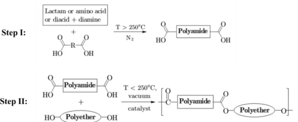
PEBA copolymers can be synthesized through different approaches. Only the typical thermal polymerization method with ester links will be briefly introduced since it represents how the specific PEBA (Pebax® from Arkema) used in this project is produced [55]. These PEBA copolymers consist of linear chains of polyamide and polyether blocks with molecular weights of about 400–3000 g/mol and 500–5000 g/mol respectively [56]. The polymerization process is carried out in two steps. Firstly, the α,ω-dicarboxylic acid terminated polyamide block is synthesized from the reaction of lactam(s), aminoacid(s) and/or diacid and diamine with a chain-terminating diacid. The average molecular weight of the resulted polyamide block is controlled by the molar ratio between the chain-terminating agent and the reactant monomers. This step is usually carried out under pressure at high temperatures. In the second step, a commercially available α,ω-dihydroxy terminated polyether reacts with the previously synthesized polyamide block to produce the designated PEBA copolymer in the presence of catalyst. A lower temperature and vacuum are used to minimize the degradation of the polyether and drive the reaction towards ester formation respectively. The two-step process is schematically shown in Fig. 2.9.

(42)

Figure 2.9: Synthesis of ester-linked PEBA copolymers through the two-step thermal polymerization (taken from Ref. [55]).

2.3.2 Solid-state Structures of PEBA

PEBA copolymers present a micro-phase separated morphology in the solid-state due to the thermodynamic incompatibility between the polyamide and polyether components (macro-phase separation is prevented by the covalent bonds between the two blocks) (Fig. 2.10). The polyamide segments crystallize into lamellar structures independently of the polyamide/polyether composition [56-59]. Barbi et al. studied solvent-cast PEBA films of various grades (polyether weight ratio varies from 53 to 80%) by SAXS [59]. They found that the layer thickness of polyamide lamellae is on the order of 6 nm and the long period ranges from 12 to 18 nm. For the rigid grades (the weight ratio of polyamide/polyether > 1), the lamellar structures can organize into spherulitic superstructures with a radius of a few microns [5].

Figure 2.10: a) Schematic representation of PEBA solid-state structures; b) TEM image of a poly(ether-b-amide) copolymer with a polyamide/polyether weight ratio of 23/77 (taken from Ref. [5, 55]).

(43)

2.4 Ion Transport in Ionically Conductive Polymers

2.4.1 Ion Transport in Block Copolymer Electrolytes

High ionic conductivity in PEO requires rapid segmental motion to accelerate ion transport, which, on the other hand, tends to decrease the rigidity of the polymer [42]. The use of PEO containing block copolymers has been shown to be a possible solution to decouple the electrical and mechanical properties, where the PEO block provides ionic conductivity and the other component(s) imparts desired mechanical properties [60]. These copolymer systems are characterized by a micro-phase separated morphology due to the thermodynamic immiscibility between the polymer blocks. The shape of the PEO microdomains can be spheres, cylinders, bicontinuous (gyroid) or lamellae, which is mainly controlled by the Flory-Huggins interaction parameter, overall degree of polymerization and the composition fraction [61, 62].

1) Effect of Morphology

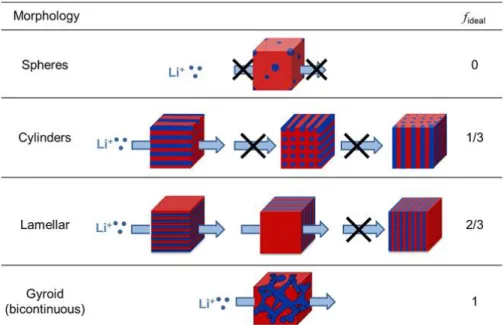
The ionic conductivity of a block copolymer electrolyte (𝜎) may be expressed as follows: 𝜎 = 𝑓𝜙𝑐𝜎0

where f is the morphology factor; 𝜙_𝑐 and 𝜎₀ are the volume fraction and intrinsic conductivity of the conducting phase, respectively. According to the work of Sax and Ottino, f can be calculated based on the morphology of the polymer electrolyte as shown in Fig. 2.11 (termed as fideal) [63]. For a spherical morphology, fideal equals 0 since no conductive pathways exist in the system. In the case of a cylindrical morphology, one-third of the grains will statistically contribute to ion transport in a certain direction and thus fideal takes a value of 1/3. Similarly, fideal equals 2/3 in a lamellar morphology and 1 in a gyroid morphology. Villaluenga et al. found that adding 2 wt% nanoparticles into lithium/polystyrene-b-poly(ethylene oxide) electrolytes resulted in an unexpected increase in conductivity [62]. Examination of the solid state structures by SAXS and STEM confirmed a morphology transition from lamella to gyroid and thus resulted in a conductivity increase. The morphology factor f was determined to be 0.94 ± 0.28 in the sample of gyroid morphology, very close to the theoretical value (fideal). Cheng et al. studied the effect of crystalline structures on ion transport in polymer electrolytes with lamellar morphology [43]. They designed a model system comprised of single PEO crystals with controlled crystal structure and size, crystallinity, and orientation. It was found that, at low ion content, the conductivity

(44)

along the lamellar plane direction can be 2000 times higher than that in the direction perpendicular to the plane due to tortuosity effects, indicating the ion transport in the system is confined within the chain fold region and is directed by the lamellar structures. However, Chintapalli et al. reported on the influence of grain size on the ionic conductivity of a block copolymer electrolyte. Surprisingly, the conductivity was decreased by a factor of 5.2 as the grain size increased from 13 to 88 nm. Results from another study also suggests that long-rang order hinders ion conductivity since ionic conductivity may be blocked by the boundaries of large grains [64].

Figure 2.11: Theoretical morphology factor fideal of polyelectrolytes with different morphologies. The blue region represents the conducting phase (taken from Ref. [62]).

2) Effect of Chain Mobility

It is generally believed that ion transport is mainly restricted within the amorphous region of a polymer electrolyte and thus should be enhanced by increasing the chain mobility. Methods to reduce the crystallinity of PEO by adding plasticizer and inorganic particles have been shown to be effective to increase the conductivity [65]. Decreasing the molecular weight is also expected to increase the ionic conductivity, which has been reported in PEO homopolymer/lithium salt complex systems [66]. However, an opposite tendency was reported in the case of block

(45)

copolymers containing PEO [45, 60, 64]. Bouchet et al. modeled the conductivity (𝜎) of the PS-PEO-PS electrolytes using the following equation [45]:

𝜎 =𝜎 0_𝜀 𝜏

where 𝜎0_{and 𝜀 are the conductivity and volume fraction of the PEO phase (a complex of pure} PEO and doped lithium slat) respectively; and 𝜏 is the tortuosity of the PEO network. They proposed that a “dead zone” of 1.6 nm independent of PEO molecular weight exists at the interface of PS/PEO where the PEO chain mobility is impeded by the covalently bonded hard PS domain (Fig. 2.12). That portion of the PEO chains does not contribute to the ion transport in the system. Similar results were also obtained in another study where the interfacial zone was estimated to be around 5 nm [64]. The argument explains the unexpected behavior in copolymer electrolytes that ionic conductivity increases with increasing PEO molecular weight, since a relatively larger portion of PEO would contribute to ion conduction as the PEO molecular weight increases [45].

Figure 2.12: Schematic representation of ion transport in the PS-PEO-PS electrolytes (taken from Ref. [45]).

2.4.2 Charge Dissipation Mechanism in PEBA Copolymers

PEBA copolymers have been widely used for antistatic applications [4, 55]. However, the charge transportation mechanism in such copolymers has not been well understood. Young and Lin studied the electrostatic dissipating properties of copolymers consisting of PEO blocks and amide groups [8]. They proposed that the PEO blocks absorb water through hydrogen bonding and the