HAL Id: hal-01799918
https://hal-mines-albi.archives-ouvertes.fr/hal-01799918
Submitted on 15 Feb 2019
HAL is a multi-disciplinary open access
archive for the deposit and dissemination of
sci-entific research documents, whether they are
pub-lished or not. The documents may come from
teaching and research institutions in France or
abroad, or from public or private research centers.
L’archive ouverte pluridisciplinaire HAL, est
destinée au dépôt et à la diffusion de documents
scientifiques de niveau recherche, publiés ou non,
émanant des établissements d’enseignement et de
recherche français ou étrangers, des laboratoires
publics ou privés.
Improvement of the bridge curvature method to assess
residual stresses in selective laser melting
Sabine Le Roux, Mehdi Salem, Anis Hor
To cite this version:
Sabine Le Roux, Mehdi Salem, Anis Hor. Improvement of the bridge curvature method to assess
residual stresses in selective laser melting. Additive Manufacturing, Elsevier, 2018, 22, p.320-329.
�10.1016/j.addma.2018.05.025�. �hal-01799918�
Improvement of the bridge curvature method to assess residual stresses in
selective laser melting
Sabine Le Roux
a,⁎, Mehdi Salem
a, Anis Hor
baInstitut Clément Ader (ICA), Université de Toulouse, CNRS, Mines-Albi, ISAE-SUPAERO, UPS, INSA, Campus Jarlard, 81013 Albi CT, CEDEX 09, France bInstitut Clément Ader (ICA), Université de Toulouse, CNRS, Mines-Albi, ISAE-SUPAERO, UPS, INSA, 3 rue Caroline Aigle, 31400 Toulouse, France
Keywords:
Selective laser melting (SLM) Bridge curvature method Distortion
Residual stresses Ti-6Al-4V alloy
A B S T R A C T
In the Selective Laser Melting (SLM) process, residual stresses are a major problem because they impact the dimensional accuracy and mechanical properties of the manufactured parts. A new methodology, based on distortion measurements using the bridge curvature method (BCM), is developed for the quantitative assessment of residual stresses. The bending of the surface of the released specimen is approximated by a quadratic poly-nomial and quantitative criteria are determined on both profiles and surface topographies measured by non-contact 3D optical microscopy. The accuracy of the method is evaluated by a statistical analysis using repeat-ability tests. Focus variation microscopy (FVM) measurements show better repeatrepeat-ability than extended field confocal microscopy. Compared to the 2D measurements generally reported in the literature, 3D characteriza-tion provides relevant informacharacteriza-tion as the orientacharacteriza-tion of the main distorcharacteriza-tion, which may help to highlight the effect of SLM process parameters. In fact, the flatness parameters and curvature attributes measured on surface topographies are much more robust and repeatable than the distortion magnitude measured on isolated profiles. In particular, 3D analysis helps to show that the distortions are maximum perpendicular to the path of the laser.
1. Introduction
Additive manufacturing (AM) processes, and in particular selective laser melting (SLM), are recognized as a promising technology due to its ability to produce complex and lightweight customized components. These are directly fabricated from a sliced 3D-CAD model, without requiring expensive part-specific tooling [1]. Despite its many ad-vantages, the SLM process is still under development, especially for aeronautical applications. Among the current challenging research to-pics, most studies focus on the material densification, microstructure and mechanical properties [2–7], while some others are dedicated to process monitoring, improving surface quality and reducing residual stresses [1,3,8–10]. The SLM process belongs to the family of powder-bed fusion (PBF) technologies [11], whereby a thin layer of powder spread on a substrate is selectively melted by a computer controlled laser beam and consolidates by heat diffusion. The part is built layer by layer, by repetition of these steps for successive powder beds [12,13]. During production, the material experiences large localized tempera-ture gradients due to rapid heating and cooling within a short time associated to the scan pattern of the high energy focused laser beam. Due to the layered build-up, the latter melting layer may re-melt or reheat the underlying layers. This results in high thermally-induced
internal stresses which can detrimentally affect the mechanical per-formances and thus the reliability and life of the components in service [14]. When removing the part from the base plate, the residual stresses are released by shrinkage and bending deformation, causing dimen-sional inaccuracies [7,9,10,15,16]. The distortion or even cracking of the part can sometimes happen during the process when the stresses reach critical levels. Understanding and controlling the development of the residual stresses inducing the component distortion is a critical issue and one of the current challenging research topics in SLM manu-facturing [1].
Residual stresses can be generated in many structures and compo-nents during various thermal or thermo-mechanical manufacturing processes such as welding, forming, heat treatment, machining, etc. [17–21]. Over the years, various techniques have been developed to evaluate residual stresses, such as X-ray and neutron diffraction, ul-trasonic velocity, magneto-acoustic emission, hole drilling, in-strumented sharp indentation, crack compliance, layer removal, etc. [22–24]. These methods can be classified depending on their char-acterization scale and their destructive or non-destructive nature. Me-chanical methods (e.g., sectioning, contour, hole-drilling, ring-core, curvature) are used to characterize type I macro-stresses which vary over large distances (namely the dimensions of the part). These
⁎Corresponding author.
E-mail addresses:sabine.leroux@mines-albi.fr(S. Le Roux),mehdi.salem@mines-albi.fr(M. Salem),anis.hor@isae-supaero.fr(A. Hor).
destructive techniques are based on the deformation measurement during or after complete or partial release of the residual stresses upon disturbing the mechanical equilibrium of the part. Non-destructive “physical” methods, such as diffraction analysis, are more relevant for assessing residual stresses of type II and type III, which occur respec-tively at the grain level or on the atomic scale [9,22]. However, the measurement uncertainties obtained by these methods depend on the material being analyzed. In particular, the correct evaluation of residual stresses in titanium alloys is difficult due to the overlap of the diffrac-tion peaks associated with their poorly defined shape [25,26].
The curvature method, which consists in measuring the deflection or curvature of a part caused by the addition or removal of material containing residual stresses, is generally used to determine post-process thermal stresses within coatings and layers [22,23,27]. It can be applied to SLM components since the additive manufacturing is based on melting of successive layers, for example to optimize process para-meters (such as laser power, scan speed and strategy, layer thickness, preheating, etc.) known to have a significant effect on the residual stresses [22,28]. Thus, several studies [13,29–32] were performed using an overhang “cantilever” test geometry selected to cause sig-nificant distortions, to investigate the influence of process parameters or to validate distortion prediction models. The method consists in determining the difference between the height of the specimen arms before and after separation from the support structure, on few points (usually about ten) along the longitudinal axis of the specimen. How-ever, the measurement accuracy is limited to a hundred or a few hun-dred micrometers, due to the method of cutting the supports, and to the high surface roughness which is not filtered in the profile [30]. In-situ measurements can be useful to monitor the PBF process during the part build [3,33,34]. Thus, Denlinger et al [35] used a laser displacement sensor to measure in situ deflection of a rectangular parallelepiped substrate material free to distort at one extremity, in order to in-vestigate the residual stresses accumulated during the building of Ti-6Al-4 V and Inconel 625 parts by laser-based directed energy deposi-tion. In addition, the authors determined the pre- and post-process plate profiles at ten points along the top of the substrate using a coordinate-measurement machine.
The changes in the plate profile and out-of-plane distortion of the substrate were then calculated by subtracting the pre-process from the post-process measurements. But this asymmetric geometry, as the cantilever, enables to assess the residual stress only in one direction, because it concentrates the stresses along the specimen axis. For their part, Kruth et al [15] investigated the amount of residual stresses in Ti-6Al-4 V parts produced by SLM using a bridge-shaped geometry speci-fically designed. Their so-called “bridge curvature method” (BCM) consists in determining the residual stress by finite elements simulation using on the curling angleα. This parameter is defined as the deviation from the normal position of the planes at the bottom of the pillars cut off from the base plate by wire EDM. It is determined using a 3D-CNC vision measuring machine. However, the measurement accuracy of the curling angle may be affected by a poor quality of the specimen cut, whereas the value of the calculated stress is very sensitive to the ac-curacy of this measure.
In the present study, an improved methodology derived from the BCM is proposed to accurately assess the part distortion of Ti-6Al-4 V bridge-shaped specimens produced by SLM. Profile and 3D surface measurements are performed on the upper surface using optical mi-croscopy before and after removing the specimen from the base plate. The surface topographies are filtered and analyzed to determine the magnitude of distortion and additional parameters expressing the shape of the curvature. The repeatability of the method is assessed by statis-tical analysis, and the results of 2D and 3D measurements are com-pared.
2. Experimental procedure 2.1. Material and specimens
SLM experiments were performed on a ProX® DMP 200 machine from PHENIX SYSTEMS. Titanium alloy Ti–6Al–4 V was used as powder material, chosen for many applications as aerospace and biomedical industries owing to its good strength-to-weight ratio, high fatigue and corrosion resistance, good bio-compatibility associated to a good formability and heat treatability [5,24]. The powder was plasma-ato-mized, resulting in a particle size ranging from 15μm to 70 μm and a median diameter d50of about 35μm. A parallelepiped bridge shape,
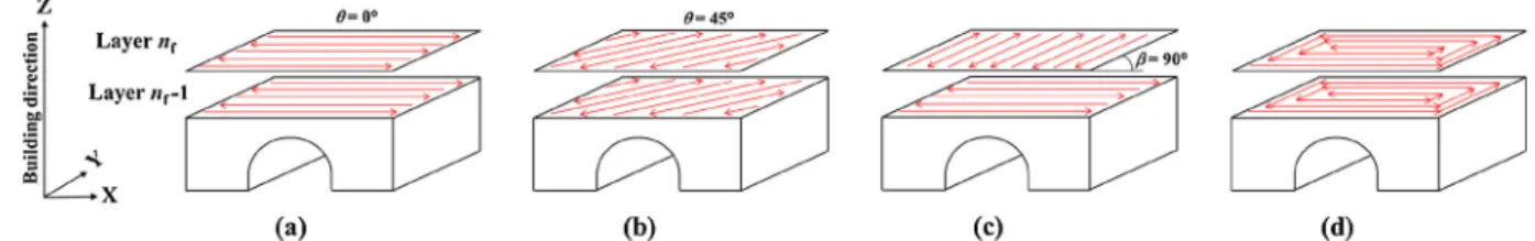
shown inFig. 1, was selected to emphasize residual stresses during and after the manufacturing [15]. Specimens were manufactured in a pro-tective argon atmosphere to prevent oxidation, using a non-preheated Ti–6Al–4 V base plate and without supporting structures. The invariant manufacturing parameters are reported inTable 1. Various laser scan strategies were investigated, as indicated inFig. 2.
2.2. Measurement of distortions
2.2.1. Non-contact optical measurement techniques
The specimens were removed from the SLM support plate by electro-erosion. The distortions due to residual stresses that developed during the building process were released during the cutting. The sur-face of the specimen was measured using an Extended Field Confocal Microscope (EFCM, Altimet AltiSurf 520), based on the principle of chromatic coding (Fig. 3a):
- focusing of a white light source reflected on the surface of the sample,
- beam splitting of the polychromatic light source into its con-stituent wavelengths by an accurate distance-measuring sensor in-corporating special chromatic lenses (each wavelength being able to focus only on a point situated at a specific distance from the sensor, thus creating a continuum of monochromatic imaging points),
- activating the distance-sensing ability of the sensor by matching the central wavelength of the reflected beam to the exact height of the
Fig. 1. Geometry and dimensions (in mm) of the SLM bridge-shaped specimen.
Table 1
Manufacturing parameters kept constant on the SLM machine.
Laser spot diameter (mm) Laser power (W) Scan speed (mm/ s) Hatch spacing (mm) Layer thickness (mm) Number of layers Contour scan 0.07 300 1800 0.085 0.06 233 none
focused point, via a spectrometer [36].
The scanning was carried out through a CHR-150 controller (Stil S.A.) connected to the profilometer and provided a topographic image representing the surface height z as a function of the surface co-ordinates (x,y). In order to improve the sensitivity of the sensor to re-flected light, dark background correction was systematically performed before measurement.
A Focus Variation Microscope (FVM, Alicona InfiniteFocus SL) was also used to measure the specimen surface. As detailed in Figure 3b, this technique is based on exploiting the small depth of focus of an optical system with vertical scanning to provide topographical and colour in-formation from the variation of focus [37]. Although less accurate on altitude coding than EFCM, this technique had the advantage here of being faster for the acquisition of large areas.
2.2.2. Profile measurements
Profile measurements were performed by EFCM on the specimen top surface in both X and Y directions, using a chromatic sensor having a 350μm depth of field (whose full features are given inTable 2). A fairly low sampling frequency of 100 or 300 Hz (depending on the specular properties of the surface) was used to limit the amount of non-measured points, which typically represented between 1 and 5% of the scanned area. Three profiles of 18.8 mm length and five profiles of 9 mm length, spaced about 4 mm apart and crossing the specimen respectively along the X and Y axes, were acquired. The profiles were spaced apart by about 4 mm. The lateral resolution of the profiles was selected to 1μm, and the measuring speed to 100μm/s in order to improve the signal. An example of a raw profile measured along X direction is given inFig. 4a. The repeatability of the measurements was evaluated on three se-lected specimens produced with different laser scan angles ϴ (i.e. 0°, 45° and 90°). Five different acquisitions were performed by the same operator, over several days/weeks. For each measurement, the spe-cimen was removed from the motorized table and then replaced.
2.2.3. Surface topographies
The topography of upper surface of the specimens (about 19.3 mm × 9.3 mm, i.e. 90% of the total area excluding extreme edges) was scanned by EFCM. Due to high z variation of the surface, a chro-matic optical probe with a large depth of field (3 mm) had to be used. A scanning speed of 1 mm/s and a low sampling frequency (100 Hz) were selected. The lateral resolution was set to 10μm along both X and Y directions to reduce the acquisition time.
Surface measurements were also carried out by FVM, chosen for its ability to measure a wide z ranges characteristic of shape defects. The specimens were mounted on a motorized stage and illuminated with ring light. A 10 × objective lens was used, giving a XY range of 22.32 mm × 11.25 mm constituted of 12 × 7 fields of view. Vertical resolution was set at 200 nm and lateral resolution at 3.9μm. Once captured, the raw height maps were cut to the same size (i.e. 19.3 mm x 9.3 mm) as surface topographies acquired by EFCM.
Using the same protocol as for the profiles, five different surface maps were scanned on each specimen to estimate the measurement repeatability with both measuring systems. In order to precisely quantify the distortions due to the residual stresses, topographic mea-surements were performed before and after separation of the parts from the base plate.
Fig. 2. Various laser scan strategies investigated: unidirectional scan pattern with a scan angle ϴ = 0° a) or 45° (b), rotating scan pattern with a hatch angleβ = 90° (c), and inward concentric scan pattern (d).
Fig. 3. Schematic diagram of topographic measuring devices: a) extended field confocal microscope (AltiSurf 520) [36]; (b) focus variation microscope (Alicona Infinite Focus) [37].
Table 2
Measuring performances of the chromatic sensors used with the extended field confocal microscope (EFCM).
Total depth of field (mm) Working distance (mm) Axial (z) resolution (μm) Lateral resolution (μm) Precision (μm) Reflection limit angle (°) 0.35 12 0.01 4 0.1 30 3 28 0.1 10 1 1
2.3. Extracting and quantifying the distortion 2.3.1. Profile processing
The raw profiles were processed using the surface metrology soft-ware Mountains Map® (DigitalSurf). The first step consisted to inter-polate non-measured points by considering the value of their nearest neighbours. Then, the profile was levelled by least mean squares (LMS) subtraction to correct the non-parallelism between the optical sensor and the surface of the specimen. To describe the bending due to the release of residual stresses, the points of the profile were fitted by a second-order polynomial function expressed as:
= = + +
z f x( ) ax2 bx c, (1)
where z is the altitude of the points of the profile, x the coordinates of these points, and a, b and c are the coefficients of the function.
The magnitude of distortion was finally assessed by calculating the parameter Pt, which corresponds to the total depth of the concave shaped curve ofFig. 4b. A sensitivity study showed that there was little difference (less than a few micrometres) in the Pt value determined using a polynomial of degree 2, 3 or even 4. On the other hand, a polynomial of higher degree (5 or more) would take into account wa-viness defects which are rather the signature of the process (for ex-ample, the weld tracks, balling, and unmelted powder). Therefore, it was decided to set the degree of the polynomial function at 2. 2.3.2. Surface topography processing
The processing procedure was the same as for profiles, except that the operations were carried out on surfaces (Fig. 5a). First, the non-measured points were interpolated and the surface levelled by LMS plane subtraction. The distortion was fitted by a quadratic polynomial surface expressed as a function of x and y as:
= = + + + + +
z f( , )x y ax2 by2 cxy dx ey f, (2)
where z is the altitude of the points of the surface, x and y are the coordinates of these points, and a, b, c, d, e and f are the coefficients of the function. Then, standardized flatness parameters such as the peak-to-valley (or total) flatness deviation FLTt and the root mean square (or quadratic) flatness deviation FLTq were calculated on the resulting surface shown in Figure 4b, without additional filtering. According to ISO 12781-1 [38], FLTt is defined as:
= +
FLTt FLTp FLTv, (3)
where FLTp is the value of the largest positive local flatness deviation from the least squares reference plane and FLTv is the absolute value of the largest negative local flatness deviation from the least squares re-ference plane.
FLTq was determined from the following equation:
∫
= FLTq A1 LFD dA, A 2 (4) where LFD represents the local flatness deviation and A the surface area of the flatness feature.FLTt was considered as the most useful flatness parameter from a metrological point of view [39].
In addition, curvature attributes were determined using a Matlab® routine. Curvature describes how much the curve deviates from straight line, in a given direction and at a particular point of the curve [40]. For a function f(x), the curvature k(x) can be expressed in terms of second derivatives as:
= +
k x( ) (1 ( f/ ) )d dxd dx2f/ 22 3/2. (5)
In a three-dimensional space defined by orthogonal (x,y,z) axes where x and y represent the map axes and z the depth axis, a surface can be described by a function z = f(x,y) which was equivalent in our case to a quadratic polynomial (Eq.1). The curvature tensor K can be ex-pressed by the following relation:
⎜ ⎟ = ⎛ ⎝ ⎞ ⎠= ⎛ ⎝ ⎜ ⎜ ⎞ ⎠ ⎟ ⎟ ∂ ∂ ∂ ∂∂ ∂ ∂ ∂ ∂∂ K KKxx KKxy . yx yy z x x yz z y x yz 2 2 2 2 2 2 (6)
The normal curvatures can be defined by planes which are ortho-gonal to the surface. The intersection of these two orthoortho-gonal planes with the surface describes the principal curvatures (Kmaxand Kmin). The
maximum curvature Kmaxand the minimum curvature Kmincorrespond
respectively to the curvatures calculated in the directions Omax and
Omin, for which the curvatures take the largest and the lowest absolute
values.
According to [30], the mean curvature Km was defined as the
average of the principal curvatures Kminand Kmax[40]:
Fig. 4. Typical raw profile levelled by LMS subtraction (a) and estimation of flatness deviation on the fitted quadratic polynomial function calculated from the raw profile (b).
= +
Km (Kmax Kmin)/2. (7)
Roberts [40] showed that the mean curvature was not particularly useful for describing the surface, since it tends to be dominated by - and consequently visually similar to - the maximum curvature Kmaxwhich
can be considered as a more meaningful attribute. However, since Km
helps to derive the principal curvatures, it can be useful to calculate its value from the coefficients of the polynomial function (Eq.2) using the following equation [41]:
= + ++ ++ −
Km a(1 (1e) db(1e)d ) cde.
2 2
2 2 3/2 (8)
Gaussian curvature Kgwas defined as the product of the principal
curvatures Kminand Kmax[40]:
=
Kg Kmin.Kmax. (9)
As for Km, this attribute has only limited applications to describe
surfaces, but is useful to derive other curvature attributes. Kgwas
cal-culated as a function of the coefficients of Eq. (2) using the following relationship [41]: = + −+ Kg (14ab cd e) . 2 2 2 2 (10) 3. Results
3.1. Repeatability of distortion measurements 3.1.1. 2D parameters
Statistical results of profile measurements by EFCM, expressed by the standard deviationσ and the coefficient of variation C.V. (or relative standard deviation, defined as the ratio of the standard deviation to the mean), are reported inTables 3 and 4respectively for the two optical probes of different ranges. First, we note that the two sensors give significantly different mean distortion magnitudes, with an average difference of 7μm in both X and Y directions. It can be considered that the 3 mm probe should be more suitable due to its greater depth of field and an axial resolution (0.1μm) sufficiently accurate to measure shape
deviations. For both sensors, profile measurements along X give C.V. of less than 8%, attesting to relatively low measurement dispersions. Higher C.V. values, close to or greater than 20%, are obtained along Y direction especially for the specimens built with ϴ = 0° and 90°.
Micrographs of the upper surface of the specimens observed with a scanning electron microscope (SEM) reveals a very coarse and hetero-geneous surface quality (Fig. 6). Surface defects such as weld tracks (appearing as ridge-like formations indicating the path followed by the laser while traversing the powder bed), spatter, unmelted and partially melted powder particles (appearing as sphere-like protrusions stuck to the surface), are clearly visible. It is well known that AM processes by powder-bed fusion produces parts with high surface roughness [8,42]
Fig. 5. Typical surface height maps measured on the top of the SLM specimens by EFCM: (a) levelled raw surface, (b) distortion defect approximated by a quadratic polynomial surface (both surfaces are represented with a normalised scale, either in top or in perspective view).
Table 3
Total magnitude of the distortion (Pt) determined on 2D profiles acquired by EFCM (with a 350μm optical sensor) on specimens removed from the base plate.
Laser scan orientation
strategy Profiledirection Mean (μm) Std. dev.(μm) C.V. (%)
ϴ= 0° X 168.8 1.85 1.09 Y 11.2 2.96 26.3 ϴ= 45° X 101.9 5.84 5.73 Y 18.4 0.84 4.57 ϴ= 90° X 56.4 2.41 4.28 Y 29.6 5.64 19.0 Table 4
Total magnitude of the distortion (Pt) determined on 2D profiles acquired by EFCM (with a 3 mm optical sensor) on specimens removed from the base plate.
Laser scan orientation Profile direction Mean (μm) Std. dev. (μm) C.V. (%)
ϴ= 0° X 178.6 2.74 1.53 Y 23.7 5.25 22.1 ϴ= 45° X 106.7 3.89 3.64 Y 11.4 0.79 6.98 ϴ= 90° X 51.3 3.73 7.28 Y 26.3 6.59 25.1
and anisotropic properties related to the laser trajectories [7,26]. This was confirmed on the investigated specimens by profile measurements carried out according to ISO 4287 [43] and ISO 4288 [44] standards, which give an arithmetic average roughness Ra ranging between 10 and 20μm depending on the scan strategy. Such surface heterogeneity can lead to uncertainty and dispersion in the mathematical fit of the poly-nomial function representative of the flatness deviation. This is parti-cularly critical when the distortion is low, as is the case with profiles along Y whose magnitude is lower to 30 μm. For the specimen built with ϴ = 45°, C.V. is of the same order of magnitude in both directions. This is related to the path of the optical probe when measuring the profiles, because the welds are crossed at 45° both in X and Y directions. 3.1.2. 3D parameters
Flatness parameters (i.e. FLTt and FLTq) and curvature attributes (Kmin, Kmax, Km,Omax) determined on surface topographies measured by
EFCM are reported inTable 5. C.V. values are less than 4% for all in-vestigated specimens, except for the minimum curvature Kmin which
exhibits a greater dispersion (3% < C.V. < 16%) probably due to the particularly low value of this attribute. One can notice the very good repeatability of the orientation Omax of the maximum curvature
(C.V. < 1%). As can be seen inTable 5, the evolution of flatness and curvatures parameters does not show the same trend as a function of the orientation of the laser scan ϴ. The reason is that curvature attributes are independent on the specimen geometry than the flatness para-meters. The second one should therefore be used preferentially when comparing experimental measurements obtained on different geome-tries.
Fig. 7a and b shows a strong similarity between the surface topo-graphies obtained by FVM and EFCM, respectively. Both reveal the specimen bending and some topographic features such as the weld tracks and unmelted particles appearing as peaks. However, the FVM surface map has a smoother appearance than the EFCM one, certainly because of a less noisy signal (with unmeasured points representing less than 0.05% of the total area). Compared to EFCM, results obtained from the Alicona FVM give slightly lower mean values for all attributes
(Table 6). This difference could be due to the lower z-resolution achieved with the principle of FVM. However, FVM provides improved measurement repeatability (C.V. ≤ 1%) except for Kminwhich is again
more scattered than other curvature attributes (C.V. up to 5%). InTable 7 are reported the calculated percentage differences be-tween the parameter mean values measured with FVM and EFCM. Re-markably low differences (≤ 3%) are observed for the two specimens with the largest distortions (i.e. ϴ = 0° and 45°), except for Kmindue to
its poorer repeatability. The differences are somewhat larger for the specimen built at 90° (between 1.7 and 11.3%), especially for the curvatures attributes Kmaxand Km. However, regarding the main
or-ientation of the distortion Omax, the difference is always very small (less
than 1%) whatever the scan orientation. This parameter can therefore be considered as particularly repeatable and robust.
3.2. Comparative measurements before and after cutting
InTable 8are reported the flatness deviations and curvature attri-butes measured by EFCM on some specimens built with various laser scan strategies (as described inFig. 2), before and after the part has been removed from the plate. In addition, the evolution of the total flatness deviation FLTt is graphically shown inFig. 8a. This graph in-dicates that before cutting, the flatness deviation is relatively low and close for all investigated specimens (FLTt = 36.5μm + /-3.3 μm). At this stage, the stress relaxation is low and concerns only the free surface layer, resulting in a small bending of the specimen. After cutting, a significant increase is observed on FLTt parameter (164μm + /-48 μm) for all scan strategies (Table 8). This increase is about 80% on average for both parameters, indicating that most of the tensile residual stresses are released after cutting, thus causing bending of the specimen.
Fig. 8b indicates that the orientation of the maximum distortion Omaxis very close to 180° (i.e. aligned with longitudinal x-axis) for all
specimens before removal from the base plate, while it varies con-siderably after cutting. An exception is however noted for the specimen built perpendicular to the X-axis (ϴ = 90°) for which Omaxremains
substantially unchanged (although with a higher curvature).
Fig. 6. SEM micrographs of the surface of the specimens built with ϴ = 0° (a) and ϴ = 45° (b), which show the weld tracks and many unmelted particles adhered on the surface.
Table 5
Flatness and curvature attributes determined on 3D topographies acquired by EFCM (with a 3 mm optical sensor) on specimens removed from the base plate.
Laser scan orientation FLTt (μm) FLTq (μm) Kmax(mm−1) Kmin(mm−1) Km(mm−1) Omax(°)
ϴ= 0° Mean 204.6 55.2 3.95 1.29 2.62 93.0 Std. dev. 4.76 0.98 0.067 0.093 0.082 0.37 C.V. (%) 2.33 1.77 1.70 7.24 3.13 0.39 ϴ= 45° Mean 180.1 37.6 3.20 0.60 1.90 125.8 Std. dev. 1.48 0.17 0.052 0.096 0.071 1.02 C.V. (%) 0.82 0.44 1.62 16.0 3.76 0.81 ϴ= 90° Mean 109.7 23.2 3.55 1.44 2.49 177.4 Std. dev. 3.55 0.69 0.12 0.047 0.072 0.31 C.V. (%) 3.24 2.98 3.38 3.29 2.90 0.18
4. Discussion
Fig. 9shows the evolution of the C.V. resulting from repeatability tests as a function of the mean value of the distortion magnitude, for both profile and surface measurements by EFCM and FVM. The re-peatability of 3D topographic measurements clearly appears much better compared to 2D profiles. In fact, the flatness and curvature parameters are statistically more representative than the magnitude of distortion estimated from one or a few isolated profiles, which depends substantially on their position on the specimen. This is particularly true on anisotropic or inhomogeneous rough surfaces such as those pro-duced by SLM. As shown by the fitted curve by a power law, the greater the deformation, the better the measurement repeatability. It will therefore be favourable to use a test geometry enabling the greatest possible deformations to be generated.
Unlike many other optical techniques that are limited to coaxial illumination, the maximum slope angle measurable by FVM does not depend solely on the numerical aperture of the lens since it can also be adjusted by the flexibility of the technique in terms of use of light (such as a ring light). This overcomes most limitations when measuring sur-faces with strongly varying reflection properties within the same field of view. This advantage has been clearly demonstrated for applications such as measurement of steep surface flanks or welding spot inspec-tions, which have a very irregular shape with steep flanks and difficult reflective behavior [37]. In our case, the SLM surfaces have many as-perities with sharp slopes (Fig. 7), leading to measurement artifacts by EFCM because of the reflection of some surface points outside the angle limit of the optical probe. This may explain the best repeatability ob-served for topographic measurements made by FVM compared to
measurements by EFCM, which is probably also related to better lateral resolution (4μm for FVM versus 10 μm for EFCM). Furthermore, ac-quisition times of surface topographies can be particularly long, typi-cally several hours with EFCM for the measurement conditions
Fig. 7. Levelled surface height maps of the specimen built with ϴ = 45°, measured by EFCM with a 3 mm optical sensor (a) and by FVM with 10 × objective (b).
Table 6
Flatness and curvature attributes determined on 3D topographies acquired by FVM (Alicona, with 10 × objective) on specimens removed from the base plate.
Laser scan orientation FLTt (μm) FLTq (μm) Kmax(mm−1) Kmin(mm−1) Km(mm−1) Omax(°)
ϴ= 0° Mean 198.2 53.7 3.84 1.38 2.61 92.2 Std. dev. 0.95 0.35 0.026 0.054 0.021 0.048 C.V. (%) 0.48 0.66 0.68 3.96 0.82 0.05 ϴ= 45° Mean 176.2 37.2 3.13 0.60 1.86 124.0 Std. dev. 1.09 0.25 0.015 0.027 0.019 0.36 C.V. (%) 0.62 0.68 0.48 4.56 1.04 0.29 ϴ= 90° Mean 103.4 22.8 3.15 1.47 2.27 178.6 Std. dev. 0.80 0.25 0.033 0.023 0.014 0.50 C.V. (%) 0.78 1.09 1.07 1.53 0.61 0.28 Table 7
Percentage difference between parameters calculated from EFCM and FVM measurements on specimens removed from the base plate.
Laser scan orientation FLTt FLTq Kmax Kmin Km Omax
ϴ= 0° 3.1 2.7 2.8 7.0 0.4 0.9
ϴ= 45° 2.2 1.1 2.2 0.0 2.1 1.4
ϴ= 90° 5.7 1.7 11.3 2.1 8.8 0.7
Table 8
Flatness deviations and curvature attributes determined before and after se-paration of the specimens from the base plate.
Laser scan
strategy Cutting FLTt (μm) FLTq (μm) K(mmmax−1) Km(mm −1) O max(°) ϴ= 0° before 37.6 7.7 1.14 0.81 174.1 after 204.6 55.2 3.95 2.62 93.0 ϴ= 90° before 34.2 8.5 2.62 1.34 178.1 after 109.7 23.2 3.55 2.49 177.4 h = 45° before 33.2 7.7 2.32 1.19 182.8 after 170.6 35.3 3.32 2.56 144.5 h = 105° before 35.0 7.7 2.10 1.18 180.1 after 116.8 24.8 2.60 2.09 196.1 Concentric inward before 39.8 8.2 2.04 1.22 179.0 after 203.3 53.5 3.80 3.01 91.6
considered in this study. FVM reduces the acquisition time to a few tens of minutes while ensuring excellent measurement repeatability, there-fore it could advantageously be used to assess the part distortion.
InFig. 9, it can also be noticed that the curve shows an inflection point corresponding to a distortion magnitude of about 35μm, which is equivalent to the median diameter d50of the Ti-6Al-4 V powder used for
manufacturing specimens. Below this distortion magnitude, C.V. ex-ceeds 5% and then increases drastically. This value can therefore be defined as the quantification limit of the developed method, below which measurements should not be relevant because of the large number of unmelted particles on the surface of SLM parts (as previously illustrated inFig. 6). Moreover, it may be thought that the presence of these particles on the surface can affect the calculation of the poly-nomial function representing the distortion. This effect was estimated by applying a morphological filter using a 70μm diameter sphere (which corresponds to the maximum size of the powder) on the surface, just before the polynomial approximation. The results showed that the value of flatness deviation parameters (FLTt and FLTq) was slightly modified (difference of less than 5%) for the distortion amplitude greater than the quantification limit.
The 3D approach provides different parameters which are very re-levant in understanding the distortion phenomena in relation to the process parameters. Besides the amplitude parameters (FLTt and Kmax),
the main orientation (Omax) of the distortion highlights the effect of the
laser scanning strategy.Fig. 10shows the distortion shapes extracted from the height maps for various scanning orientations ϴ. It reveals that Omaxcoincide with the vertical axis (at x = 10 mm) only for ϴ = 0°
(Fig. 10a), while the axis of bending changes when ϴ departs from 0°
(Figs. 10b and c). Since the residual stresses are generated mainly along the laser scan direction, the resulting distortion is oriented perpendi-cular to ϴ. Parry et al [45] recently established through thermo-me-chanical simulation that the greatest stress component develops parallel to the scan vectors.
Changing the orientation of the laser scanner varies not only Omax,
but also the distortion magnitudes along X and Y, without however reversing the values by varying ϴ from 0° to 90° (Tables 3 and 4). The difference in distortion amplitude along X and Y is inherent to the asymmetric geometry of the bridge specimen (whose length is twice as large as its width). This geometry naturally promotes bending at the thinnest area of the specimen, i.e. along X-axis (as illustrated in Fig. 10a). Thus, the distortion magnitude along X for ϴ = 0° remains higher than along Y for ϴ = 90°. In addition, the maximum deforma-tion is induced by a unidirecdeforma-tional laser scan along the x-axis (ϴ = 0°) which also leads to the longest scan vectors, while the minimal de-formation is observed for ϴ = 90° which exhibits the shortest scan vectors (Fig. 8a). Several experimental and numerical works [9,15,28,29,46] have reported a link between the length of the scan vectors and the residual stresses. These considerations further underline the relevance of 3D measurements, since the resulting parameters (especially Omax) make it possible to better explain and correlate the
results with the process parameters, that would not be from simple profile measurements. It must be emphasized that all the results dis-cussed above were obtained on the specimens removed from the base plate.
Measurements made on the specimens prior to separation from the support plate revealed much smaller distortion magnitudes than after cutting (about 80% lower). Moreover, the distortion amplitude before cutting is close to the quantification limit allowed by the measurement method (35μm). This distortion can be neglected in the present study, since the distortion after cutting reflects the total released residual stresses. However, the distortion before cutting should be considered when its magnitude is significant, and this in order to precisely corre-late the distortions with the residual stresses. Based on a numerical model developed to predict the distortion of SLM manufactured parts, Li et al [13] found that the tensile stress in a cantilever specimen de-creased of 70% when it was removed from the support. With this kind of geometry, the distortion is relatively high before cutting and must be taken into account.
As previously shown (Fig. 8b), the orientation of the distortion be-fore cutting seems independent of the scan strategy (Omaxclose to 180°
whatever the laser scan orientation, the hatch angle, etc.). In fact, the orientation of the main deformation Omaxcorresponds to the maximum
curvature Kmax, which represents the deflection rate over a given length
(Eq.5). Since profile measurements along X and Y revealed that before cutting, the distortion amplitudes are very close in both directions, and the geometry of the bridge specimen is asymmetric (X = 2Y), then the
Fig. 8. Evolution of the total flatness deviation FLTt (a) and of the orientation Omaxof the main curvature (b) of specimens built with various scan strategies, before and after removal from the base plate.
Fig. 9. Evolution of the coefficient of variation versus the mean distortion magnitude (all data determined from profile and surface measurements are represented).
curvature Kmaxis logically maximum in the direction (Y). It is only after
cutting that the impact of the orientation of the weld seams on Omaxis
effective. A comprehensive investigation to determine the effect of laser scan strategy on residual stresses and validate these assumptions is planned.
5. Conclusions
A new method, based on the bridge curvature method (BCM) and non-contact optical measurements of the specimen surface (by EFCM or FVM), was developed to assess the distortions for application to SLM manufactured parts. Repeatability tests revealed that measurements on 3D surface topographies are more robust than 2D profile measurements. An excellent repeatability was obtained in particular on surface height maps measured by FVM. However, surface defects such as unmelted powders can affect the measurement accuracy of the distortion when its magnitude is less than 40μm, which corresponds to the median size of
the powder particles.
Compared to 2D methods and associated criteria reported in the literature, flatness deviation parameters (such as FLTt and FLTq) and curvature attributes (such as the mean curvature Kmor the maximum
curvature Kmax) proposed in our approach are more reliable as
re-presentative of the overall deformation of the specimen. In addition, the 3D approach makes it possible to have a better knowledge of the de-formation distribution on the specimen, and especially to determine unambiguously the maximum distortion and its associated orientation. It was also shown that, before the specimen was removed from the base plate, the flatness deviation remains low and quasi-independent of the scan strategy, while it increases on average by 80% after cutting of the specimen.
This methodology can be applied to study the effect of process parameters such as the laser scan strategy and the part geometry on deformations and residual stresses, using bridge-shaped specimens or any other type of specimen (such as cantilever) provided that it has a
Fig. 10. 3D height maps showing the distribution of the distortion for different laser scan orientations ϴ, after removing the specimen from the base plate: a) ϴ = 0°, c) ϴ = 45°, d) ϴ = 90° (the white dotted line indicates the main orientation of the distortion ϴmax).
flat upper surface. The 3D mapping of the surface deformation could also help validate thermo-mechanical simulation of the process used to predict residual stresses and distortions in SLM manufactured parts. Acknowledgments
The authors would like to thank the CIRIMAT for providing SLM specimens. Kévin Grondin is greatly acknowledged for its contribution to the development of the Matlab® routine.
References
[1] S. Bremen, W. Meiners, A. Diatlov, Selective laser melting, a manufacturing tech-nology for the future, Laser Technik J. 9 (2) (2012) 33–38.
[2] J.-P. Kruth, G. Levy, F. Klocke, T.H.C. Childs, Consolidation phenomena in laser and powder- bed based layered manufacturing, CIRP Ann. Manuf. Technol. 56 (2) (2007) 730–759.
[3] M. Mani, B. Lane, A. Donmez, S. Feng, S. Moylan, R. Fesperman, Measurement Science Needs for Real-Time Control of Additive Manufacturing Powder Bed Fusion Processes, US Department of Commerce, National Institute of Standards and Technology, NISTIR, 2015, p. 8036.
[4] S. Leuders, M. Thöne, A. Riemer, T. Niendorf, T. Tröster, H.A. Richard, H.J. Maier, On the mechanical behaviour of titanium alloy TiAl6V4 manufactured by selective laser melting: fatigue resistance and crack growth performance, Int. J. Fatigue 48 (2013) 300–307.
[5] L.C. Zhang, H. Attar, Selective laser melting of titanium alloys and titanium matrix composites for biomedical applications: a review, Adv. Eng. Mater. 18 (4) (2016) 463–475.
[6] Y.J. Liu, S.J. Li, H.L. Wang, W.T. Hou, Y.L. Hao, R. Yang, T.B. Sercombe, L.C. Zhang, Microstructure, defects and mechanical behavior of beta-type titanium porous structures manufactured by electron beam melting and selective laser melting, Acta Mater. 113 (2016) 56–67.
[7] M. Simonelli, Y.Y. Tse, C. Tuck, Effect of the build orientation on the mechanical properties and fracture modes of SLM Ti–6Al–4V, Mater. Sci. Eng. A 616 (2014) 1–11.
[8] A. Townsend, N. Senin, L. Blunt, R.K. Leach, J.S. Taylor, Surface texture metrology for metal additive manufacturing: a review, Prec. Eng. 46 (2016) 34–47. [9] P. Mercelis, J.P. Kruth, Residual stresses in selective laser sintering and selective
laser melting, Rapid Prototyp. J. 12 (5) (2006) 254–265.
[10] C.R. Knowles, T.H. Becker, R.B. Tait, Residual stress measurements and structural integrity implications for selective laser melted Ti-6Al-4V, S. Afr. J. Ind. Eng. 23 (3) (2012) 119–129.
[11] A.S.T.M. ASTM, F2924-14, Standard Specification for Additive Manufacturing Titanium-6 Aluminum-4 Vanadium With Powder Bed Fusion, ASTM Standards, 10.04, (2014),http://dx.doi.org/10.1520/F2924.
[12] N. Keller, F. Neugebauer, H. Xu, V. Ploshikhin, Thermo-mechanical simulation of additive layer manufacturing of titanium aerospace structures, Proc. DGM Int. Congr. Light Mater. (2013).
[13] C. Li, J.F. Liu, Y.B. Guo, Z.Y. Li, Efficient multiscale prediction of cantilever dis-tortion by selective laser melting, Proc. 27th Annual International Solid Freeform Fabrication Symposium – An Additive Manufacturing Conference, University of Texas, Austin, USA, 2016, pp. 236–246. August 8-10.
[14] N.S. Rossini, M. Dassisti, K.Y. Benyounis, A.G. Olabi, Methods of measuring residual stresses in components, Mater. & Des. 35 (2012) 572–588.
[15] J.P. Kruth, J. Deckers, E. Yasa, R. Wauthlé, Assessing and comparing influencing factors of residual stresses in selective laser melting using a novel analysis method, Proc. Inst. Mech. Eng. Part. B: J. Eng. Manuf. 226 (6) (2012) 980–991. [16] B. Cheng, S. Shrestha, K. Chou, Stress and deformation evaluations of scanning
strategy effect in selective laser melting, Addit. Manuf. 12 (2016) 240–251. [17] P.J. Withers, Residual stress and its role in failure, Rep. Prog. Phys. 70 (12) (2007)
2211.
[18] R.H. Leggatt, Residual stresses in welded structures, Int. J. Press. Vessel. Pip. 85 (3) (2008) 144–151.
[19] K. Masubuchi, Analysis of Welded Structures: Residual Stresses, Distortion, and Their Consequences vol 33, Elsevier, 2013.
[20] M. Kleiner, R. Krux, W. Homberg, Analysis of residual stresses in high-pressure sheet metal forming, CIRP Ann. Manuf. Technol. 53 (1) (2004) 211–214. [21] B.R. Sridhar, G. Devananda, K. Ramachandra, R. Bhat, Effect of machining
para-meters and heat treatment on the residual stress distribution in titanium alloy
IMI-834, J. Mater. Process. Technol. 139 (1) (2003) 628–634.
[22]P.J. Withers, H.K.D.H. Bhadeshia, Residual stress. Part 1–measurement techniques, Mater. Sci. Technol. 17 (4) (2001) 355–365.
[23]F.A. Kandil, J.D. Lord, A.T. Fry, P.V. Grant, A Review of Residual Stress Measurement Methods, A Guide to Technique Selection, NPL, Report MATC (A), (2001), p. 4.
[24]X. Wang, K. Chou, Residual stress in metal parts produced by powder-bed additive manufacturing processes, Proc. 26th Annual International Solid Freeform Fabrication Symposium – An Additive Manufacturing Conference, University of Texas, Austin, USA, 2015, August 10-12, 2015, pp. 1463–1474.
[25]K. Moussaoui, S. Segonds, W. Rubio, M. Mousseigne, Studying the measurement by x-ray diffraction of residual stresses in Ti6Al4V titanium alloy, Mater. Sci. Eng. A 667 (2016) 340–348.
[26]N. Dai, L.C. Zhang, J. Zhang, X. Zhang, Q. Ni, Y. Chen, M. Wu, C. Yang, Distinction in corrosion resistance of selective laser melted Ti-6Al-4V alloy on different planes, Corr. Sci. 111 (2016) 703–710.
[27]M. Larsson, P. Hedenqvist, S. Hogmark, Deflection measurements as method to determine residual stress in thin hard coatings on tool materials, Surf. Eng. 12 (1) (1996) 43–48.
[28]J.P. Kruth, L. Froyen, J. Van Vaerenbergh, P. Mercelis, M. Rombouts, B. Lauwers, Selective laser melting of iron-based powder, J. Mater. Process. Technol. 149 (1) (2004) 616–622.
[29]M.F. Zaeh, G. Branner, Investigations on residual stresses and deformations in se-lective laser melting, Prod. Eng. 4 (1) (2010) 35–45.
[30]D. Buchbinder, W. Meiners, N. Pirch, K. Wissenbach, J. Schrage, Investigation on reducing distortion by preheating during manufacture of aluminum components using selective laser melting, J. Laser Appl. 26 (1) (2014) 012004.
[31]L. Papadakis, A. Loizou, J. Risse, J. Schrage, Numerical computation of component shape distortion manufactured by selective laser melting, Procedia CIRP 18 (2014) 90–95.
[32]I. Yadroitsava, S. Grewar, D. Hattingh, I. Yadroitsev, Residual stress in SLM Ti6Al4V alloy specimens, Mater. Sci. Forum 828 (2015) 305–310.
[33]G. Tapia, A. Elwany, A review on process monitoring and control in metal-based additive manufacturing, J. Manuf. Sci. Eng. 136 (2014) 060801.
[34]S.K. Everton, M. Hirsch, P. Stravroulakis, R.K. Leach, A.T. Clare, Review of in-situ process monitoring and in-situ metrology for metal additive manufacturing, Mater. Des. 95 (2016) 431–445.
[35]E.R. Denlinger, J.C. Heigel, P. Michaleris, T.A. Palmer, Effect of inter-layer dwell time on distortion and residual stress in additive manufacturing of titanium and nickel alloys, J. Mater. Process. Technol. 215 (2015) 123–131.
[36] J. Cohen-Sabban, J. Gaillard-Groleas, P.J. Crepin, Quasi-confocal extended field surface sensing, Proc. SPIE 4449, Optical Metrology Roadmap for the Semiconductor, Optical, and Data Storage Industries II, 178, December 10, 2001, pp. 178–183, ,http://dx.doi.org/10.1117/12.450093.
[37]R. Danzl, F. Helmli, S. Scherer, Focus variation–a robust technology for high re-solution optical 3D surface metrology, Strojniški vestnik-J, Mech. Eng. 57 (3) (2011) 245–256.
[38]ISO_12781-1:2011 Geometrical Product Specifications, (GPS) — flatness — part 1: vocabulary and parameters of flatness, International Organization for
Standardization, Geneva, 2011.
[39]K. Nadolny, W. Kapłonek, Analysis of flatness deviations for austenitic stainless steel workpieces after efficient surface machining, Meas. Sci. Rev. 14 (4) (2014) 204–212.
[40]A. Roberts, Curvature attributes and their application to 3D interpreted horizons, First Break 19 (2) (2001) 85–100.
[41]K. Rektorys, Differential Geometry, in: Survey of Applicable Mathematics, Iliffe Books Ltd, MIT Press, Cambridge, MA, 1969, pp. 298–373.
[42]R. Leach, Metrology for additive manufacturing, Meas. Control 49 (4) (2016) 132–135.
[43]B.E. ISO_4287, BS EN ISO_4287. Geometrical Product Specification (GPS) Surface Texture: Profile Method Terms, Definitions and Surface Texture Parameters, British Standards Institute, 2000.
[44]B.E. ISO_4288, BS EN ISO_4288. Geometric Product Specification (GPS) Surface Texture Profile Method: Rules and Procedures for the Assessment of Surface Texture, British Standards Institute, 1998.
[45]L. Parry, I.A. Ashcroft, R.D. Wildman, Understanding the effect of laser scan strategy on residual stress in selective laser melting through thermo-mechanical simulation, Addit. Manuf. 12 (2016) 1–15.
[46]N. Keller, V. Ploshikhin, New method for fast predictions of residual stress and distortion of AM parts, Proc. 25th Annual International Solid Freeform Fabrication Symposium, University of Texas, Austin, USA, 2014, pp. 1229–1237. August 4-6.