Parsimonious variational-Bayes mixture aggregation with a Poisson prior

(1)

HAL Id: inria-00383945

https://hal.inria.fr/inria-00383945

Submitted on 13 May 2009

HAL is a multi-disciplinary open access

archive for the deposit and dissemination of

sci-entific research documents, whether they are

pub-lished or not. The documents may come from

teaching and research institutions in France or

abroad, or from public or private research centers.

L’archive ouverte pluridisciplinaire HAL, est

destinée au dépôt et à la diffusion de documents

scientifiques de niveau recherche, publiés ou non,

émanant des établissements d’enseignement et de

recherche français ou étrangers, des laboratoires

publics ou privés.

Parsimonious variational-Bayes mixture aggregation

with a Poisson prior

Pierrick Bruneau, Marc Gelgon, Fabien Picarougne

To cite this version:

Pierrick Bruneau, Marc Gelgon, Fabien Picarougne. Parsimonious variational-Bayes mixture

aggrega-tion with a Poisson prior. European Signal Processing Conference (Eusipco’2009), Aug 2009, Glasgow,

United Kingdom. pp.280-284. �inria-00383945�

(2)

PARSIMONIOUS VARIATIONAL-BAYES MIXTURE AGGREGATION

WITH A POISSON PRIOR

Pierrick Bruneau, Marc Gelgon and Fabien Picarougne

Nantes university, LINA (UMR CNRS 6241), Polytech’Nantes

rue C.Pauc, La Chantrerie, 44306 Nantes cedex 3, France

INRIA Atlas project-team

firstname.surname@univ-nantes.fr

ABSTRACT

This paper addresses merging of Gaussian mixture models, which answers growing needs in e.g. distributed pattern recog-nition. We propose a probabilistic model over the parameter set, that extends the weighted bipartite matching problem to our mixture aggregation task. We then derive a variational-Bayes associated estimation algorithm, that ensure low cost and parsimony, as confirmed by experimental results.

1. INTRODUCTION

This paper addresses the issue combining several probabilis-tic mixture models of a single process. It focuses on the case input and output models are Gaussian mixture models (GMM), as this semi-parametric form is one of the most em-ployed and versatile tool for modelling the density of mul-tivariate continuous features. Alternatively, the same mix-ture scheme may be used for clustering data into Gaussian-shaped classes, in which case our task consists in a search for a consensus between data partitions. Whether for density estimation or clustering, our goal is to build a mixture that optimally describes the mixture ensemble. Both its parame-ters and number of components should be determined.

Aggregation of class models is a classical topic, both su-pervised (ensemble methods) and unsusu-pervised. Growing interest comes from the transposition of existing statistical learning and recognition tasks onto distributed computing systems (cluster, P2P), which has motivated parsimonious model aggregation techniques [7], or sensor network.

A combined model could simply be obtained by a weighted sum of Gaussian mixtures, yet this would generally result in an unnecessarily high number of Gaussian components, with a view to capturing the underlying probability density. The scope of the paper is a new scheme for estimating, from such a possibly over-complex mixture, a mixture that is more par-simonious, yet preserves the ability to describe the underly-THIS WORK WAS PARTLY FUNDED BY ANR SAFIMAGE (FRENCH MINISTRY OF UPPER EDUCATION AND RESEARCH) AND REGION PAYS DE LA LOIRE (MILES PROJECT)

ing generative process. Parsimony is particularly important if such mixture combinations follow one after another.

A straightforward solution would consist in sampling data from this combined mixture and re-estimating a mixture from this data, but this is generally not cost effective, especially in high dimensional spaces. Yet, this is interesting as a bench-mark. In contrast, our technique operates on the sole pa-rameters of the over-complex mixture papa-rameters, ensuring lower cost for computation and communication, should the scheme operated in a distributed setting. In fact, our tech-nique seeks an optimal combination of Gaussian components, taking into account which mixture their arise from. By em-ploying a Bayesian formulation of the over-complex mixture parameter estimation and a variational approach to its reso-lution, the amount of compression and the suitable combina-tion of Gaussian components may be jointly determined.

Gaussian mixture simplification through crisp combina-tion of Gaussian components may, for small-size problems, be addressed through the Hungarian method to obtain a glob-ally optimal combination. Lower cost, local optima have been sought in [5], where the authors seek a combination that minimizes an approximation of Kullback-Leibler loss. Their technique may be viewed as a kind of k-means op-erating over components, or a bipartite matching resolution between 2 sets of Gaussian components. As an alternative, a procedure akin to ascendent hierarchical clustering operat-ing on Gaussian components is proposed in [8]. The search space considered in [9] is richer, as linear combinations of components are sought, rather than binary assignments, cor-responding to a shift from k-means to maximum likelihood and EM operating on Gaussian components. However, these works leave open the central issue of the criterion and pro-cedure for determining the desirable number of components. Bayesian estimation of mixture models is a well-known principle to solving the above issue, especially model com-plexity. In particular, the variational resolution provides a good trade-off between accuracy and computation efficiency, with a procedure known as Variational Bayes-EM [1] (VBEM hereafter). Yet, the standard use of VBEM is applied to data

(3)

in Rn.

The central contribution of our paper is to define and demonstrate how simplification of an over-complex mixture may be carried out effectively by extending the Variational Bayes-EM principles to handling Gaussian components in-stead of real vectors. Besides conjugate priors on mixture pa-rameters, the proposed probabilistic model includes a Pois-son prior that discourages merges between Gaussian compo-nents supplied by the same mixture. This improves explo-ration of the search space significantly, i.e. reduces compu-tation cost, over the simpler option of ignoring the origin of components in the reduction process.

Section 2 describes how the VBEM framework can be extended to parameter level, to conduct Bayesian clustering of Gaussian components. Section 3 extends this proposal by adapting the probabilistic model and deriving the asso-ciated estimation algorithm, including an initialization strat-egy. Section 4 provides experimental results and draws con-cluding remarks.

2. TRANSPOSING VARIATIONAL BAYESIAN TO PARAMETERS

Variational Bayesian EM framework is an iterative density modeling and clustering scheme based on a joint probabil-ity distribution function (pdf ) defined over all variables and model parameters. Parameter modeling (a.k.a prior model-ing) regularizes obtained estimates. More precisely, singu-larities are avoided, and the output number of significant (i.e. different from prior) components is as low as sensible [1, 3]. The joint distribution is defined by the following set of

where X is a d-dimensional data set, Z the latent vari-ables associating X with one of the K components in the

model, θ = {θk}, θk = {πk, µk,Λk}, π = {πk}, µ =

{µk}, Λ = {Λk} are the model parameters, and {αk, βk, νk, Wk}

are the hyper-parameters (0 indices denoting prior values). Generally, prior parameters and hyper-parameters are set to uninformative values. Posterior values are obtained as an output.

This scheme was combined [4] with virtual samples [10] in order to merge and reduce a set of Gaussian mixtures. These mixtures might come from various sources and their addition involve high redundancy. Using this procedure (named VBMerge hereafter) we build a parsimonious and sensible representative.

Introducing virtual samples modifies the pdf s over X and Z. Let us remark that through virtual samples, the orig-inal distribution over X now depends solely on the input

model θ′ = {θ′

l}, θl′ = {πl′, µ′l,Λ′l} (i.e. the set of

Gaus-sian mixtures to reduce).

ln p(X | Z, µ, Λ) = N 2 K X k=1 L X l=1 zlkπ′l[ln det Λk− Tr(ΛkΛ ′₋₁ l ) − (µ′ l− µk)TΛk(µ′l− µk) − d ln(2π)] (5) p(Z | π) = N Y n=1 K Y k=1 πznk k = L Y l=1 K Y k=1 πN π′lzlk k (6)

3. REDUCING A GAUSSIAN MIXTURE UNDER CONSTRAINTS

Let us consider several data repositories, each one being the source of a Gaussian mixture fitted on the available data. The previously proposed method [4] makes a weighted sum of all components from all sources in a single large mixture, and reduces it. Yet, doing so with a large number of sources has a drawback : as we obtain a globally very noisy model, the number of components is reduced drastically (see experi-mental results). Should we assume that each source produces a non-redundant Gaussian mixture, it would be sensible to penalize reductions that imply assigning components origi-nating from the same source to the same target component.

Consequently, let us design a probabilistic model and de-rive the associated estimation algorithm, that takes into ac-count this constraint to tackle the mixture merging question efficiently. Consider that the L components come from P

distinct sources (necessarily, L ≥ P ). We denote alp the

binary variable that denotes wether component l originates

from source p or not. Let us define A the L× P matrix

formed with alpvalues. As we know where each component

originates from, A is a set of observed values.

We define a pdf over this new data set. The purpose of such a distribution is to model how much assignments of the L components violate or enforce the constraints defined by A, so it is sensible to restrict A dependencies to Z. Further-more, A can be seen as originating from this distribution ; an assignment configuration (summarized by Z) enforcing the constraints would therefore result in a higher likelihood for the model. Before introducing the distribution, let us

con-sider the P× K matrix M = AT_{Z. One of its single terms}

mpkmeasures how many components from a single source

(4)

we want this amount to be as low as possible, so we model this constraint with a Poisson distribution parametrized with

λ= 1 over each term. This will tend to favor rare events.

Thus the pdf over A is as follows :

p(A|Z) = p(M = ATZ) = P Y p=1 K Y k=1 e−1 (1 + mpk)! (7) The term 1 is added for conveniency, and causes no loss of generality. The new global joint distribution is obtained

by incorporating (7) to the set of pdf s{ (3), (4), (5) , (6) }.

The classical VBEM algorithm (and its derivations) are based on two essential elements : updating estimates, and controlling convergence through a lower bound value. Read-ers are encouraged to see ([3] chapter 10) for thorough im-plementation details and theoretical justifications. We will focus on terms involving Z hereafter.

Let q(Y ) be a factorized variational distribution so that

q(Y ) =Q

jqj(Yj), and X a set of observed variables. Then

the optimal factor q_j∗w.r.t. others kept fixed is obtained as :

ln qj∗(Yj) = Ei6=j[ln p(X, Y )] + const (8)

Let us deriveln q∗_{(Z) for our modified joint distribution:}

ln q∗(Z) = Eπ,µ,Λ[ln p(A, X, Z, π, µ, Λ)] + const (9)

ln q∗_{(Z) = E}

π[ln p(Z|π)] + Eµ,Λ[ln p(X|Z, µ, Λ)]

+ ln p(A|Z) + const (10)

Following classic derivation ([3] chapter 10) adapted to the virtual sample context [10, 4], we obtain :

ln q∗_{(Z) = N} L X l=1 K X k=1 zlkπl′ [ln ˜πk+ 1 2ln ˜Λk− d 2ln(2π) − 1 2[ d βk + νkTr(WkΛ′−1_l ) + νk(µ′l− mk)TWk(µ′l− mk)]] − K X k=1 P X p=1 ln(1 + mpk)! + const (11) Or, equivalently : ln q∗_{(Z) =} L X l=1 K X k=1 zlkln ρlk− K X k=1 P X p=1 mpk X i=0 ln(1+i)+const (12) with ln ρlk = N π′l[ln ˜πk+ 1 2ln ˜Λk− d 2ln(2π)− 1 2[ d βk + νkTr(WkΛ′−1l ) + νk(µ′l− mk)TWk(µ′l− mk)]] (13) ˜

πk = E[ln πk], and ˜Λk= E[ln det Λk]

Let us denote z.kthe set{zlk| ∀l} (and respectively zl.).

In the traditional scheme,ln q∗_{(Z) factorizes over l and k,}

giving rise to independent optimal zlk estimates (more

pre-cisely, only unnormalized estimates are fully independent :

each zlkultimately depends on ρl.in order to obtain

normal-ized values rlk). Here this does not hold any more. All zlk

forming a single z.kare co-dependent : we must devise an

alternate to the traditional E step.

We choose to define an order in the set of individuals, and approximate the overall co-dependent estimates by a one-pass scheme based on using already discovered estimates. This leads to the following approximation :

q(Z) = q(z1.)q(z2.|z1.)q(z3.|z1.z2.) . . . q(zL.|z1.. . . zL−1.)

(14) Our E step algorithm will proceed each term of the r.h.s. in increasing ranks order. We will describe the 2 first steps of the algorithm, leading to a general formulation. This it-erated conditional scheme is closely related to ICM (itit-erated conditional modes) [2].

3.1. Initializing the scheme

Let us recall that mpk =PLl=1alpzlk. Our formulation

al-lows us to restrict this sum to the current rank of the algo-rithm. For the first step we have :

ln q∗_(z 1.) = K X k=1 z1kln ρ1k− K X k=1 P X p=1 ln(1 + a1pz1k) + const (15)

For a single z1k, this leads to :

ln q∗(z1k) = z1kln ρ1k−

P

X

p=1

ln(1 + a1pz1k) + const (16)

Clearly, as such, this expression cannot give a multino-mial law estimate. However, using a first order Taylor

ex-pansion forln(1 + x), we obtain :

ln q∗(z1k) = z1kln ρ1k− P X p=1 a1pz1k+ const (17) ln q∗(z1k) = z1kln ρ1k ePPp=1a1p + const (18)

As each original component belongs to only one source,

ln q∗(z1k) = z1kln

ρ1k

e + const (19)

Giving a modified unnormalized estimate ρ′1k = ρ

1k

e .

This leads to the same normalized estimates as in the classi-cal scheme (e denominator is constant and disappears).

(5)

3.2. A new general update formula forln q∗_(Z)

Changing the rank of the restriction in eq. 15 leads to :

ln q∗_(z 2.|z1.) = K X k=1 z2kln ρ2k− K X k=1 P X p=1 ln(1 + a1pz1k) − K X k=1 P X p=1 ln(1 + a1pz1k+ a2pz2k) + const (20) After considering a single k, and applying Taylor expansion supplies: ln q∗_(z 2k|z1k) = z2kln ρ2k− P X p=1 a1pz1k − P X p=1 (a1pz1k+ a2pz2k) + const (21)

Let us note aimax= arg maxpaipand zimax = arg maxkzik.

Using these notations, the previous expression can be factor-ized as following :

ln q∗_(z

2k|z1k) = z2k(ln ρ2k−1−2δa1max,a2max.δz1max,k)+const

(22) where δ is the Kronecker delta. This leads to a modified unnormalized estimate :

ρ′_2k= ρlk

e1+2δa1max,a2max.δz1max,k

For any rank, same considerations lead to the following general formula :

ρ′_jk= ρjk

e1+Pj−1i=1(j−i+1).δaimax,ajmax.δzimax,k

(23) where j is the rank of the current item (i.e. original compo-nent).

3.3. Modified bound

The bound is defined by a sum of expectations w.r.t the cur-rent variational distribution [3]. For it to be complete, we need to add a term associated to the distribution we intro-duced. The modified bound additional term is the following:

E[ln p(A | Z)] = K X k=1 P X p=1  −1 − E[mpk] X i=0 ln(1 + i)   (24) = −KP − K X k=1 P X p=1 E[mpk] X i=0 ln(1 + i) (25) with E[mpk] = E " _L X l=1 alpzlk # = L X l=1 alpE[zlk] = L X l=1 alprlk (26)

In the classical VBEM scheme, this lower bound is strictly increasing during the estimation process. As we chose an approximate heuristic for our modified E step, this property does not hold any more : slight decreases can therefore be observed. But this does not change the principle of the

al-gorithm : we still can use∆(bound) < threshold as a stop

criterion, the only difference being that now∆ might be

neg-ative.

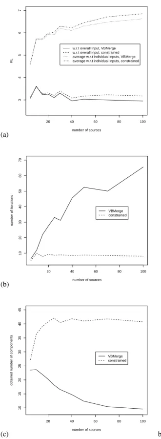
4. EXPERIMENTS AND CONCLUSION We selected the 10 first categories in the Caltech-256 ob-ject category dataset [6], thus forming a set of 1243 images. We consider each image as a data source, and fit a Gaussian mixture over its pixel data ((L,a,b) color space, augmented by the pixel positions (x,y)). Obtained individual Gaussian mixtures comprise 18.1 components on average. We then randomly select x sources from the pool of images and per-form the reduction. We measure :

• the KL divergence of the reduced model w.r.t. the overall input (i.e. superimposed Gaussian mixtures), and w.r.t. each individual data source,

• the number of iterations before convergence,

• the number of significant components in the obtained model.

Results are reported in figure 1 for various numbers of input sources (i.e. images). From these results we draw the following conclusions :

• the new technique provides reduced models that are equivalent to those of the baseline method, in the KL divergence sense. Occasionally, a slight loss was ob-served compared to the baseline method.

• as expected, our method prevents undesirable drastic reduction of the model : when reducing a set of 100 data sources (i.e. 1800 components on average), we obtain 40 components instead of 9. We see the ”noise” effect on the results with VBMerge : as more and more components are considered, we introduce noise, which sometimes leads to simplistic reductions. The new technique thus supplies a trade-off between keep-ing the original structure and a slight signal loss. • as the number of data sources increases, our method

proves much faster than the baseline method. More precisely, the baseline method convergence becomes slower as the number of data sources augments. Intu-itively, for the baseline method a lot of computational time is used to perform drastic reductions (leading to low improvements in terms of KL divergence), while in the new scheme, constraints allow us to stop the process as soon as possible.

(6)

(a) 20 40 60 80 100 3 4 5 6 7 number of sources KL

w.r.t overall input, VBMerge w.r.t overall input, constrained average w.r.t individual inputs, VBMerge average w.r.t individual inputs, constrained

(b) 20 40 60 80 100 10 20 30 40 50 60 70 number of sources number of iterations VBMerge constrained (c) 20 40 60 80 100 10 15 20 25 30 35 40 45 number of sources

obtained number of components

VBMerge constrained

b

Figure 1: a : KL divergence of the reduced models w.r.t. the input sources, b : number of iterations before convergence, c : number of components in the reduced models.

Let us add a remark about algorithmic complexity : VB-Merge iterations complexity is o(L), while for the constrained derivation it is o(L ln(L)). But on figure 1, we note that the number of iterations for VBMerge is linear w.r.t. L, while for our derivation it becomes o(1). The loss for a single iteration is therefore largely outweighed by the gain in convergence time.

As a conclusion, we have proposed a novel scheme for merging Gaussian mixtures based on a variational-Bayes pro-cedure. Introduction of the Poisson prior shows to signifi-cantly improve speed performance.

5. REFERENCES

[1] H. Attias. A variational Bayesian framework for graph-ical models. Advances in Neural Information Process-ing Systems - MIT Press, 12, 2000.

[2] S. Basu, M. Bilenko, A. Banerjee, and R. J. Mooney. Probabilistic semi-supervised clustering with

con-straints. In Semi-Supervised Learning. MIT Press,

2006.

[3] C. M. Bishop. Pattern Recognition and Machine

Learning. Springer, New York, 2006.

[4] P. Bruneau, M. Gelgon, and F. Picarougne. Parameter-based reduction of Gaussian mixture models with a variational-Bayes approach. In 19th International Con-ference on Pattern Recognition, 2008.

[5] J. Goldberger and S. Roweis. Hierarchical clustering of a mixture model. Advances in Neural Information Processing Systems - MIT Press, 17, 2004.

[6] G. Griffin, A. Holub, and P. Perona. Caltech-256 object category dataset. Technical Report 7694, California In-stitute of Technology, 2007.

[7] A. Nikseresht and M. Gelgon. Gossip-based computa-tion of a Gaussian mixture model for distributed mul-timedia indexing. IEEE Transactions on Mulmul-timedia, (3):385–392, March 2008.

[8] A. Runnalls. A Kullback-Leibler approach to Gaus-sian mixture reduction. IEEE Trans. on Aerospace and Electronic Systems, 2006.

[9] N. Vasconcelos. Image indexing with mixture hierar-chies. Proceedings of IEEE Conference in Computer Vision and Pattern Recognition, 1:3–10, 2001. [10] N. Vasconcelos and A. Lippman. Learning mixture

hi-erarchies. Advances in Neural Information Process-ing Systems - MIT PressNeural Information ProcessProcess-ing Systems, II:606–612, 1998.