HAL Id: hal-01347798
https://hal.archives-ouvertes.fr/hal-01347798
Submitted on 15 Apr 2020
HAL is a multi-disciplinary open access
archive for the deposit and dissemination of
sci-entific research documents, whether they are
pub-lished or not. The documents may come from
teaching and research institutions in France or
abroad, or from public or private research centers.
L’archive ouverte pluridisciplinaire HAL, est
destinée au dépôt et à la diffusion de documents
scientifiques de niveau recherche, publiés ou non,
émanant des établissements d’enseignement et de
recherche français ou étrangers, des laboratoires
publics ou privés.
A hybrid approach for probabilistic relational models
structure learning
Mouna Ben Ishak, Philippe Leray, Nahla Ben Amor
To cite this version:
Mouna Ben Ishak, Philippe Leray, Nahla Ben Amor. A hybrid approach for probabilistic relational
models structure learning. 15th International Symposium on Intelligent Data Analysis (IDA 2016),
2016, Stockholm, Sweden. �10.1007/978-3-319-46349-0_4�. �hal-01347798�
structure learning
Mouna Ben Ishak1, Philippe Leray2, and Nahla Ben Amor1
1 LARODEC Laboratory, ISG, Universit´e de Tunis, Tunisia
2 DUKe research group, LINA Laboratory UMR 6241, University of Nantes, France
Abstract. Probabilistic relational models (PRMs) extend Bayesian networks (BNs) to a relational data mining context. Just like BNs, the structure and parameters of a PRM must be either set by an expert or learned from data. Learning the struc-ture remains the most complicated issue as it is a NP-hard problem. Existing approaches for PRM structure learning are inspired from classical methods of learning the BN structure. Extensions for the constraint-based and score-based methods have been proposed. However, hybrid methods are not yet adapted to re-lational domains, although some of them show better experimental performance, in the classical context, than constraint-based and score-based methods, such as the Max-Min Hill Climbing (MMHC) algorithm. In this paper, we present an adaptation of this latter to relational domains and we made an empirical evalua-tion of our algorithm. We provide an experimental study where we compare our new approach to the state-of-the art relational structure learning algorithms. Keywords: Probabilistic relational model, Relational structure learning, Rela-tional Max-Min Hill Climbing
1 Introduction
Probabilistic relational models (PRMs) [9,16] are an extension of Bayesian networks (BNs) [15] which allow to work with relational database representation rather than propositional data representation. PRMs are interested in manipulating structured rep-resentation of the data, involving objects described by attributes and participating in relationships, actions, and events. The probability model specification concerns classes of objects rather than simple attributes.
In order to be used, PRMs have to be constructed either by an expert or using learn-ing algorithms. PRM learnlearn-ing implies findlearn-ing a graphical structure as well as a set of conditional probability distributions that fit the best way to the relational training data. PRM structure learning remains the most challenging issue, as it is considered as a NP-Hard problem [7]. Only few works have been proposed to learn PRMs [6] or al-most similar models [12,13,10] from relational data. Proposed algorithms are inspired from standard BNs learning approaches. Those latter are divided into three families, namely, constraint-based, score-based and hybrid approaches [5]. PRM structure learn-ing approaches are adaptations of either constraint-based or score-based approaches. However, it has been shown that, for BNs, some hybrid approaches provide better ex-perimental results than constraint-based and score-based methods [17]. In this paper we
present a new hybrid algorithm to learn the structure of a PRM from a complete rela-tional dataset. Our proposal is an adaptation of the Max-Min Hill Climbing (MMHC) algorithm [17]. We call it Relational Max-Min Hill Climbing algorithm, RMMHC for short. Also, we provide an experimental study where we compare the RMMHC algo-rithm to state-of-the-art methods. The remainder of this paper is as follows: Section 2 presents useful background and discusses related work. Section 3 details the RMMHC algorithm. Section 4 provides the empirical study. Finally, Section 5 concludes and out-lines some perspectives.
2 Background
We start by providing a brief recall on PRMs and presenting methods to learn BNs and PRMs structure from data.
2.1 Probabilistic Relational models
A PRM is defined through two components: a graphical one, a dependency structure defined over the attributes of a relational structure (i.e., an entity-relationship model or a relational schema) containing classes ans class attributes, and a numerical component that quantifies probabilistic dependencies between variables of the relational structure. Relational model. A relational structure consists of a set of classes X ≡ E ∪ R, where E is a set of entity classes and R is a set of relationship classes. Each R ∈ R links a
set of entity classes R(Ei. . . Ej). Each X ∈ E ∪ R has a set of attributes denoted by
A(X). Every attribute takes on a range of values V(X.A).
A relational skeleton σ is a partial specification of an instance of a relational structure. It specifies the set of class objects that exist in a domain and the relations that hold between them.
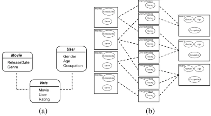
Example 1. An example of a relational structure is depicted in Figure 1(a), with three classes X = {Movie, V ote, User}. E = {Movie, User}. R = {V ote} The entity class User has three attributes A(User) = {Gender, Age, Occupation}. The linked entities of the relationship V ote are Movie and User (Dotted links).
Figure 1(b) shows an example of a relational skeleton for the relational schema of Fig-ure 1(a). It consists of three User objects and five Movie objects. User user1 has voted for two movies M = movie1 and movie2.
Probabilistic model. A PRM M = (S, Θ) brings together the strengths of proba-bilistic graphical models and the relational representation of data. A dependency struc-ture S is constructed by adding probabilistic dependencies between class attributes,
∀X.A ∈ A(X), there is a set of parents P a(X.A) = {U1, . . . , Ul}. The numerical
component is composed of the conditional probability distributions (CPD) of the at-tributes in the context of their parents in the dependency structure P (X.A|P a(X.A)). Probabilistic dependencies may be intra or inter classes, this depends on the path that connects the child to its parent. Several paths may be found depending on the way how the relational structure has been traversed. Friedman et al. [6] specify the path between
Movie User Vote Movie User Gender Age Occupation ReleaseDate Genre User Rating (a) Rating Age Gender Occupation user1 User1,movie1 Age Gender Occupation user2 Age Gender Occupation user3 Rating User1,movie2 Rating User2,movie1 Rating User2,movie2 Rating User2,movie3 Rating User3,movie2 Rating User3,movie3 Rating User3,movie4 Genre ReleaseDate movie1 Genre ReleaseDate movie2 Genre ReleaseDate movie3 Genre ReleaseDate movie4 (b)
Fig. 1: Example of a relational structure (a) and a relational skeleton (b) for the movie domain inspired from the MovieLens dataset http://grouplens.org/ datasets/movielens/ Movie User ReleaseDate Genre Age Gender Occupation User.Gender M F 0.4 0.6 Vote Rating Movie.Genre Votes.Rating Low High Drama, M 0.5 0.5 Drama, F 0.3 0.7 Horror, M 0.2 0.8 Horror, F 0.9 0.1 Comedy, M 0.5 0.5 Comedy, F 0.6 0.4 U s e r. G e n d e r (a) Rating Age Gender Occupation user1 User1,movie1 Age Gender Occupation user2 Age Gender Occupation user3 Rating User1,movie2 Rating User2,movie1 Rating User2,movie2 Rating User2,movie3 Rating User3,movie2 Rating User3,movie3 Rating User3,movie4 Genre ReleaseDate movie1 Genre ReleaseDate movie2 Genre ReleaseDate movie3 Genre ReleaseDate movie4 (b)
Fig. 2: Example of a probabilistic relational model (a) and a ground graph (b) for the movie domain of Figure 1
the parent and child variables using a slot chain. Heckerman et al. [8] refer to as con-straint and Maier et al. [12] call it relational path.
Moreover, depending on the cardinality (i.e., the number of items an entity can par-ticipate in a relationship), it is possible for an attribute object to have multiple parents objects (i.e., a Many cardinality). This number of parents is finite but not known in ad-vance and it varies from one object to another. Whereas, there is only one CPD shared among all objects of a given parent attribute X.A. To address this issue, the notion of aggregation has been adopted from database theory: An aggregate γ takes a multiset of values of some ground type, and returns a summary of it. γ can be the MAX, MIN, MODE, etc.
Each parent Ui has then the form X.B if it is a simple attribute in the same class.
Example 2. Figure 2(a) shows a PRM for the relational structure of Figure 1(a).
U ser.Occupationhas two parents from the same class User. V ote.Rating has two
parents: V ote.User.Gender from the User class and V ote.Movie.Genre from the
M ovie class. V ote.Movie.genre → V ote.rating is an example of a probabilistic
dependency derived from a path of length one where V ote.Movie.genre is the parent and V ote.rating is the child as shown by Figure 2(a). Also, varying the path length may give rise to other dependencies. For instance, using a path of length three, we can have a
probabilistic dependency from γ(V ote.User.User−1.M ovie.genre)to V ote.rating.
In this case, V ote.rating depends probabilistically on an aggregate value of all the genres of movies rated by a particular user.
Given a PRM M and a relational skeleton σ, we can construct a ground Bayesian network (GBN) by applying the probabilistic dependencies specified in M to the object attributes of σ. The CPD for each x.A is inherited from the CPD P (X.A|P a(X.A)) defined in the PRM. An example of the graphical structure of a GBN is shown by Figure 2(b).
2.2 From BN to PRM structure learning
A wealth of literature has been produced that seeks to understand and provide methods for BN structure learning from data [5]. Some of the proposed approaches have been extended to learn from relational domains. In this section we start by a brief survey on BN structure learning approaches, then we present existing approaches for PRM struc-ture learning.
BN structure learning. is known as an NP-Hard problem [3]. BN structure learning methods are divided into three main families. The first family tackles this issue as a constraint satisfaction problem. Constraint-based algorithms look for independencies (dependencies) in the data, using statistical tests then, try to find the most suitable graphical structure with this information. The second family treats structure learning as an optimization problem. They evaluate how well the structure fits to the data using a score function. So, these Score-based algorithms search for the structure that max-imizes this function. The third family presents hybrid algorithms which combine the main features of both techniques, for instance, by using local conditional independence tests and global scoring functions. Tsamardinos et al. [17] proposed the max-min hill climbing (MMHC) hybrid algorithm and provided a wide comparative study among several algorithms from three algorithm families, using several benchmarks and met-rics (e.g., execution time, SHD measure). Following this study, they showed that their proposal outperforms other algorithms included in the study. The MMHC algorithm consists of two phases:
– The first phase, ensured by the max-min parents and children (MMP C) algorithm, aims to find, for each node in the graph, the set of candidate nodes that can be con-nected to it. At this stage there is no distinction between children and parents nodes and links orientation is not of interest. MMP C discovers the set of candidate par-ents and children (CPC) for a target variable T . It consists of a raw neighborhood identification step ensured by the MMP C algorithm and an additional symmet-rical correction step, where MMP C removes from each set CP C(T ) each node
Xfor which T /∈ CP C(X). MMP C consists of a forward phase where for each variable T of the graph, a set of variables are added to CP C(T ), and a backward phase whose role is to remove false dependencies detected in the forward phase. Dependency is measured using an association measurement function such as
mu-tual information or χ2.
– The second phase allows the construction of the graph G using the greedy search heuristic constrained to the set of candidate parents and children of each node re-sulting from the first phase.
PRM structure learning. aims at finding the dependency structure S for a given rela-tional structure and a relarela-tional observarela-tional dataset that instantiates this structure. As we have seen in Section 2.1, paths may be arbitrary large and give rise to complicated
models. So that a user specified value, a maximum path length (Kmax), is required to
limit the length of possible paths that one can cross in the model. Only few works have been proposed to learn PRM structure from relational data [6,12,13,10]. These latter are inspired from classical methods for BN structure learning.
Friedman et al. [6] proposed the Relational Greedy Hill-Climbing Search (RGS)
al-gorithm. For each path length k ∈ {0, Kmax} RGS defines a hypothesis space of
potential PRM structures (i.e., neighbors) it is willing to consider, using the add edge,
delete edgeand reverse edge operators. Then, it computes the score of each
neigh-bor, and keeps the graph that has the best score, until it reaches a structure that has the highest score in the list of neighbors. As score function, they used a relational extension of the Bayesian Dirichlet (BD) score [4]. In this process, the neighborhood search space could be super-exponential.
Maier et al. proposed two constraint-based approaches. The first is a relational exten-sion of the PC algorithm to learn PRM structure from relational data [13]. Yet, unlike the PC algorithm which is sound and complete the RP C algorithm did not satisfy these criteria. The second approach comes to refine the RP C algorithm [12]. They proposed the relational causal discovery (RCD) algorithm and proved that this approach is sound and complete for causally sufficient relational data. The RCD algorithm performs on two phases. In the first phase, given a maximum path length, RCD starts by providing the set of all potential dependencies. Then continues by removing conditional inde-pendences found using conditional independence tests. Because of asymmetry caused by the use of aggregate functions, RCD verifies whether a statistical association is detected between two variables in both directions and it leaves the dependency if a statistical association exists in at least one direction, but omits this information about orientation. In the second phase, RCD determines the orientation of the dependencies discovered previously. Orientation rules are similar to those used by the P C algorithm. In [10] the authors proposed a refined version of the RCD algorithm in term of time complexity and space.
Hybrid approaches combine both techniques and some algorithms, such as the MMHC, experimentally outperforms the classical approaches. Yet, no hybrid algorithm has been proposed for PRMs. In the next section, we will provide a new hybrid approach to learn PRM structure from relational data. Our proposal is a relational extension of the
M M HCalgorithm detailed at Section 2.2, that we refer to as relational max min hill
A hybrid approach for Probabilistic Relational Models structure learning 7
Algorithm 1 RMMP C
Require: schema: A relational model, D: A database instance Current P ath length: A path length, T : A target attribute
Ensure: CP C: The set of parents and children of T , CP C(T ) = CP Csym T ∪ CP C
asym T
1: P otlist= Generate potential list(T, Current P ath length)
% Phase I: Forward 2: repeat
3: hF.assocF i = MaxMinHeuristic(T, CP C(T ), P otlist)
4: if assocF 6= 0 then
5: if Current path length = 0 OR does Not Contains Many Relationship(F ) then 6: CP Csym T = CP C sym T ∪ F 7: else 8: CP CTasym= CP C asym T ∪ F 9: end if 10: CP C(T ) = CP CTsym∪ CP C asym T 11: P otlist= P otlist\F 12: end if
13: until CPC has not changed or assocF = 0 or P otlist=∅
% Phase II: Backward 14: for all A ∈ CP C(T ) do
15: if ∃S ⊆ CP C, s.t.Ind(A; T |S) then 16: CP C(T ) = CP C(T )\{A} 17: end if
18: end for
Consequently, each parent is a variable, while each target is an attribute. When search-ing the CP C(T ), T is a target attribute. CP C(T ) consists of the candidate parents and children of T , and |CP C(T )| depends on the length of the traversed path k ∈ {0 . . . Kmax}. For each value of k, a subset of potential parents and children can be
generated. As the final generated CP C(T ) list may be very large, we adopt the same strategy as [8] and we proceed by phases. That is, suppose that we want to provide the list of children and parents of each attribute T given a maximum path length kmax, the
neighborhood identification will be done on kmax+1phases. At phase 0, we will search
for the set of parents and children of attribute T from the same class as T , at phase 1, we will search for the set of parents and children of attribute T in classes related to T class using paths of length one. At phase 2, we will go through further classes and search for the set of parents and children of attribute T in classes related to T class by traversing paths of length 2 and so on. The neighborhood identification, for one specified value of path length, is described by Algorithm 3. The Generate potential list method aims to identify the list of potential parents and children of a target attribute T given a path length k. Its result is a set of potential variables defined as follows:
– XT.A, for intra-class dependencies.
– XT.k.Y.Aor γ(XT.k.Y.A), this set presents inter-class dependencies. With respect
to the definition of a PRM (cf. Section 2), XT.k.Y.Aand γ(XT.k.Y.A)could only
be parents of the target attribute T .
3 RMMHC: The Relational Max Min Hill Climbing Algorithm
RM M HCpreserves the same phases as the MMHC algorithm (cf. Section 2.2). The
neighborhood identification phase, ensured by the RMMP C algorithm, handles asym-metry caused by the use of aggregators and leads to a partially oriented neighborhood (cf. Section 3.1). This latter is then used to simplify the global structure identification phase (cf. Section 3.2).
3.1 Relational Max Min Parents and children: RMMP C
Neighborhood identification: RMMP C. The RMMP C algorithm aims to find the list of neighbors of a target attribute T , that consists of either children or parents of T , from a set of potential variables. For BNs, MMP C does not make a difference between a node in the graph structure and a variable, and the potential set of parents and children of a node T is V\T , where V is the set of BN nodes. While, in a relational domain, and due to the horizon of crossed paths, the number of potential variables is not fixed. Thus, we have to make the difference between an attribute and a variable:
– An attribute is characterized by its name, domain, a set of possible aggregators and the class that it belongs to. A child is an attribute.
– A variable is characterized by its name, domain, the class that it belongs to, a spe-cific aggregator type and the path that it is derived from. A parent is a variable and its path starts from the class to which the child belongs. This notion is defined in [12] as a canonical dependency.
Algorithm 2 RMMP C
Require: schema: A relational model, D: A database instance, Current P ath length: A path length, T : A target attribute
Ensure: CP C: The set of parents and children of T , CP C = CP Csym
∪ CP Casym
1: if Current P ath length = 0 then 2: CP CsymT =∅, CP C asym T =∅ 3: CP C(T ) = CP Csym T ∪ CP C asym T 4: end if
5: CP C(T ) = RMMP C(schema, D, T, Current P ath length) 6: for all A ∈ CP C(T ) do
7: if Current P ath length = 0 then 8: CP Csym A =∅, CP C asym A =∅ 9: CP C(A) = CP CAsym∪ CP C asym A 10: end if
11: CP C(A) = RM M P C(schema,D, A, Current P ath length) 12: if A ∈ CP Csym
T AND T /∈ CP CAsymthen
13: CP C(T ) = CP C(T )\{A} 14: end if
15: end for
the RGS procedure, using the relational Bayesian score (cf. Section??). In this case, P otK(X.T )consists of the CP C list of variable X.T found on the local search step.
As this set contains two subsets, the choice of the operator to be performed during the neighbors generation process will depends on the concerned subset:
– For CP Csym
T : each A ∈ CP C
sym
T can be either a child or a parent of X.T so all
the operators, namely, add edge, delete edge and reverse edge can be tested. – For CP Casym
T : each A ∈ CP C
asym
T is a potential parent of X.T so only the
add edgeand delete edge operators can be tested.
The global search step is expensive in term of complexity, since the size of the generated neighborhood may increase rapidly. In the standard MMHC, the MMP C result is used as input for the GS algorithm. In the relational context both the local and global search procedures are included in an iterative process which increases the path length where we look for possible probabilistic dependencies between variables and till we reach a maximum value of the path length which is user-defined. RMMHC performs the local search procedure in phases until reaching Kmax. The result of this search
procedure will be the CP C list of all variables for all path lengths. This result is the input of the global search procedure that will be run only one time. The overall process is as presented in Algorithm??.
3.3 Time complexity of the algorithms
The MMP C algorithm consists of the MMP C algorithm of complexity O(|P otlist| .2|CP C|)
and an additional symmetrical correction. Thus, its overall complexity is O(|P otlist|2.2|CP C|).
At each iteration of the classical greedy search algorithm, the number of possible local
Consequently, each parent is a variable, while each target is an attribute. When search-ing the CP C(T ), T is a target attribute. CP C(T ) consists of the candidate parents and children of T , and |CP C(T )| depends on the length of the traversed path k ∈
{0 . . . Kmax}. For each value of k, a subset of potential parents and children can be
generated. As the final generated CP C(T ) list may be very large, we adopt the same strategy as [6] and we proceed by phases. That is, suppose that we want to provide the
list of children and parents of each attribute T given a maximum path length kmax, the
neighborhood identification will be done on kmax+1phases. At phase 0, we will search
for the set of parents and children of attribute T from the same class as T , at phase 1, we will search for the set of parents and children of attribute T in classes related to T class using paths of length one. At phase 2, we will go through further classes and search for the set of parents and children of attribute T in classes related to T class by traversing paths of length 2 and so on. The neighborhood identification, for one specified value of path length, is described by Algorithm 1. The Generate potential list method aims to identify the list of potential parents and children of a target attribute T given a path
length k. Its result is a set of potential variables of the form XT.Afor intra-class
de-pendencies and XT.k.Y.Aor γ(XT.k.Y.A)for inter-class dependencies.
On the other hand, as some dependencies may require aggregators, there is an inherent asymmetry and this list of candidate dependencies is closely related to the path com-position. So that, we propose to divide the neighborhood list, CP C, into two sub-lists.
Formally, CP C(T ) = CP Csym
T ∪ CP C
asym
T , where:
– CP Csym
T :The set of potential children and parents of target attribute T coming
either from the same class as T , with path length equal to 0 or from paths that do not contain any Many relationship.
– CP Casym
T :The set of potential variables coming from the other paths. In this case,
Acould only be a potential parent of T [7].
As for the standard case [17], MaxMinHeuristic selects the variables that maximize the MinAssoc with target attribute T conditioned to the subset of the currently
esti-A hybrid approach for Probabilistic Relational Models structure learning 11
Algorithm 3 RMMHC
Require: schema: A relational model, D: A database instance, kmax:
M aximun P ath Length
Ensure: The local optimal dependency graph S % Local search
1: for Current P ath length = 0 to kmaxdo
2: for all T do
3: CP C(T ) = RM M P C(schema,D, T, Current P ath length) 4: end for
5: end for % Global search
6: S = RGS(schema, D, CP C)
changes is bounded by O(V2), where V is the number of variables in the graph [?].
Our RMMP C algorithm presents the same steps as for the standard case, augmented with the Generate potential list procedure which is of complexity O(Nk), where
Nis the number of classes and k is the current path length. Thus, its time complex-ity, at each k value, k ∈ {0 . . . Kmax} remains equal to O(|P otlist| .2|CP C|). Thus,
augmented with the symmetrical correction, the time complexity of the RMMP C al-gorithm is O(|P otlist|2.2|CP C|). For RGS, we have to iterate on variables and for each
variable, we have to iterate on the list of all potential parents of this variable. Unlike the standard case where this set is fixed for all nodes of the graph, the relational context makes this set variable, depending on the length of the considered path. A probabilistic dependency is no longer a simple link between two nodes in a graph, but a link from a possible path. Let us consider β the number of potential parents that could be reached, then the number of possible local changes is bounded by O(β.V). Note that β = |CP C| when the RGS is called after a local search step performed using RMMP C algorithm. In RMMHC algorithm, the local search step has been augmented with an outer loop presenting the current path length to consider at each iteration. Thus the final complex-ity of the local search is O(Kmax.|P otlist|2.2|CP C|).
3.4 RMMHC vs related work
RGS defines a hypothesis space of potential PRM structures (i.e., neighbors) it is will-ing to consider, computes the score of each neighbor, and keeps the graph that has the best score, until it reaches a structure that has the highest score in the list of neigh-bors. In this process, the neighborhood search space could be super-exponential. Our RM M HCalgorithm treats this issue via its local search phase. RMMP C provides information regarding the neighborhood, which allows to reduce the size of the search space during the global structure identification phase and enhance the scalability. In contrast to the RCD approach, the asymmetry caused by the use of aggregators can provide more interesting interpretation than dependency detection. Clearly, if an inde-pendence is detected in both directions then we can conclude that these two variables are independent. Otherwise, if a dependence is detected in one direction and not in the other, the semantic of the path involved in this dependency may even provide a
deci-mated CP C(T ) = CP Csym
T ∪ CP C
asym
T .
Symmetrical correction: RMMP C. The RMMP C algorithm (Algorithm 2) comes to refine the result of Algorithm 1 by applying a symmetrical correction to the RMMP C result. As CP C(T ) consists of two subsets, the symmetrical correction depends on the concerned subset.
– For each A ∈ CP Csym
T , we must verify that T ∈ CP C
sym
A , otherwise, A has
to be removed from CP Csym
T . This symmetrical correction is equivalent to the
symmetrical correction of standard MMP C.
– For each A ∈ CP Casym
T , we cannot apply the symmetrical correction since the
SQL queries involved in such a case are not equivalent and the resulting datasets on
which we will apply statistical tests are not the same. However, ∀A ∈ CP Casym
T ,
Acan only be a parent of T . By this way, we can deduce the dependency direction,
directly from the first phase of RMMHC.
A detailed toy example on the various steps of this phase can be found in [1]. 3.2 Global structure identification
The global structure identification is performed using a score-based algorithm only on the set of variables derived from the first local search phase. We choose to work with the
RGSprocedure, using the relational Bayesian score. In this case, P otK(X.T )consists
of the CP C list of attribute X.T found on the local search step. As this set contains two subsets, the choice of the operator to be performed during the neighbors generation process depends on the concerned subset:
– For CP Csym
T : each A ∈ CP C
sym
T can be either a child or a parent of X.T so all
the operators, namely, add edge, delete edge and reverse edge can be tested.
– For CP Casym
T : each A ∈ CP C
asym
T is a potential parent of X.T so only the
add edgeand delete edge operators can be tested.
The global search step is expensive in term of complexity, since the size of the generated neighborhood may increase rapidly. RMMHC performs the local search procedure in
phases until reaching the Kmax value. The result of this search procedure will be the
500 1000 1500 2000 2500 3000 0.0 0.2 0.4 0.6 0.8 1.0 sample size A v er age (h/s)−Precision RGS RCD RMMHC
(a) Average precision
500 1000 1500 2000 2500 3000 0.0 0.2 0.4 0.6 0.8 1.0 sample size A v er age (h/s)−Recall RGS RCD RMMHC (b) Average recall 500 1000 1500 2000 2500 3000 0.0 0.2 0.4 0.6 0.8 1.0 sample size A v er age (h/s)−F−Measure RGS RCD RMMHC (c) Average F-measure
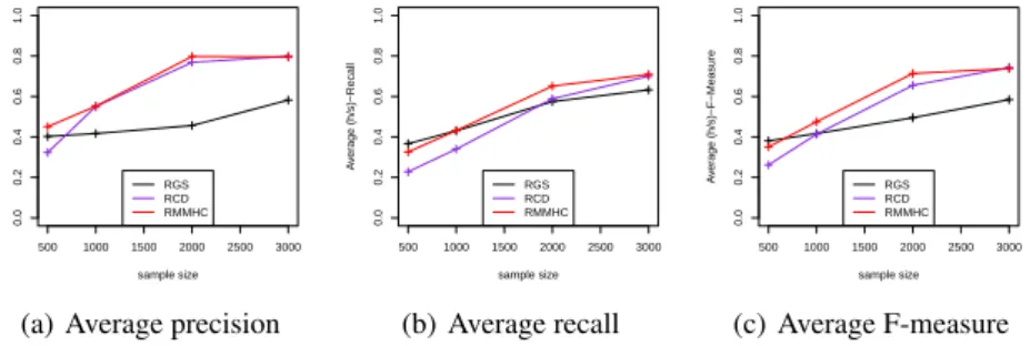
Fig. 3: The average values of Precision, Recall and F-Measure with respect to the sam-ple size
further reduce the size of the search space during greedy search. It is used as input to the global search procedure that will be run only one time. The overall process is as presented by Algorithm 3.
3.3 Time complexity of the algorithms
The MMP C algorithm consists of the MMP C algorithm of complexity O(|P otlist| .2|CP C|)
and an additional symmetrical correction. Thus, its overall complexity is O(|P otlist|2.2|CP C|).
At each iteration of the classical greedy search algorithm, the number of possible local
changes is bounded by O(V2), where V is the number of nodes in the graph [17].
Our RMMP C algorithm presents the same steps as for the standard case, augmented
with the Generate potential list procedure which is of complexity O(Nk), where
N is the number of classes and k is the current path length. Thus, its time
complex-ity, at each k value, k ∈ {0 . . . Kmax} remains equal to O(|P otlist| .2|CP C|). Thus,
augmented with the symmetrical correction, the time complexity of the RMMP C
al-gorithm is O(|P otlist|2.2|CP C|). For RGS, we have to iterate on attributes and for
each attribute, we have to iterate on the list of all its potential parents. Let us consider β the number of potential parents that could be reached, then the number of possible local changes is bounded by O(β.V). Note that β = |CP C| when the RGS is called after a local search step performed using RMMP C algorithm. In RMMHC algorithm, the local search step has been augmented with an outer loop presenting the current path length to consider at each iteration. Thus the final complexity of the local search is
O(Kmax.|P otlist|2.2|CP C|).
4 Experiments
We will compare the RMMHC algorithm to the state-of-the-art approaches, namely, the RGS and RCD algorithms (cf. Section 2.2). The RCD is supposed to correct the theoretical problems of RP C and an experimental study on these two approaches can be found in [12]. Thus the RP C algorithm is excluded from the comparative study. In
term of specific implementations, we have re-implemented the RGS algorithm and used our version in the experimental study. We have used the source code of the RCD
algo-rithm available in3. As both RCD and RMMHC use statistical independence tests,
we have implemented the linear regression test to fit the RCD implementation and we have used it to perform statistical tests during the local search phase of RMMHC. To judge conditional independence, we have run both RCD and RMMHC using a threshold α = 0.05.
Networks and Datasets. Unlike standard Bayesian networks, where a set of ground truth models (i.e., benchmarks) is available to perform experimentations, there is no such models defined in the context of PRMs. Consequently, we have used our gener-ating process, already described in [2] to generate gold models and relational database instances. We have followed the same experimental protocol as [12] and we have gener-ated relational models containing: 4 entity classes, one less than the number of entities as relationship classes. The number of attributes per class is drawn from P oison(λ =
1) + 1and cardinalities are selected uniformly at random. The number of
dependen-cies is from 1 to 15, limited by a maximum path length = 3 and at most 3 parents per variable. For each of the previously described networks, we have randomly sampled 5 relational observational complete datasets with 500, 1000, 2000 and , 3000 instances as an average number of objects per class for each.
Evaluation metrics. We have compared the algorithms in term of the quality of recon-struction. using the Precision, Recall and F-score measurement defined in [12]. Experimental results. Figure 3 presents the experimental results in term of Preci-sion, Recall and F-score. RGS presents the worst result for all sample sizes ≥ 1000.
RM M HCoutperforms RGS and RCD in term of Precision for all sample sizes and
it presents the best Recall and F-score values for sample sizes ≥ 1000. For small sam-ple size (= 500), RMMHC and RGS have similar results, followed by the RCD algorithm. Figure reft4 shows that for sample size ≥ 1000, beyond 50% of the de-pendencies retrived by RMMHC are relevant. Figure 3(b) shows that for sample size ≥ 1000, RMMHC was able to find beyond 40% of the relevant dependencies. Both values are increased by raising the sample size.
5 Conclusion
We proposed a first hybrid approach to learn PRMs structure from relational observa-tional data. Our RMMHC algorithm is based on a local search phase that allows to handle asymmetry and leads to a partially oriented neighborhood. This latter is used as input to simplify the global structure identification phase, optimize the search space and consequently enhance the scalability. We have also presented a first comparative study of state-of-the-art relational structure learning approaches and experiments showed that our approach presents good results in term of quality of reconstruction. However, this work is just the beginning for several challenging research tasks.
RM M HC can be improved to deal with more complex structural uncertainty [7], or
it can be adapted to learn PRM extensions [14]. Another avenues for future research is
combining other theories to learn the model structure [11]. Also, one interesting per-spective consists on the use of some prior knowledge, derived from knowledge repre-sentation frameworks such as ontologies, as input to the learning process.
References
1. Ben Ishak M.: Probabilistic relational models: learning and evaluation. Ph.D. dissertation, Universit´e de Nantes, Ecole Polytechnique; Universit´e de Tunis, Institut Sup´erieur de Gestion de Tunis, (2015)
2. Ben Ishak M., Leray P., Ben Amor N.: Probabilistic relational model benchmark generation: Principle and application. Intelligent Data Analysis International Journal (to appear), 615– 635, (2016)
3. Chickering D. M., Geiger D., Heckerman D.: Learning Bayesian networks is NP-hard. Tech-nical report, MSR-TR-94-17, Microsoft Research, (1994)
4. Cooper G.F., Herskovits, E.: A Bayesian method for the induction of probabilistic networks from data. Machine Learning, 9, 309–347, (1992)
5. Daly R., Shen Q., Aitken S.: Learning Bayesian networks: approaches and issues. The Knowl-edge Engineering Review, 26, 99–157, (2011)
6. Friedman N., Getoor L., Koller D., Pfeffer A.: Learning probabilistic relational models. In Proceedings of the International Joint Conference on Artificial Intelligence, pp. 1300–1309, (1999)
7. Getoor L., Koller D., Friedman N., Pfeffer A., Taskar B.: Probabilistic Relational Models. In Getoor, L., and Taskar, B., eds., Introduction to Statistical Relational Learning, MA: MIT Press, Cambridge, (2007)
8. Heckerman D., Meek C., Koller D.: Probabilistic models for relational data, Technical report, Microsoft Research, Redmond, WA, (2004)
9. Koller D., Pfeffer A.: Probabilistic frame-based systems. In Proc. AAAI, pp. 580–587, AAAI Press, (1998)
10. Lee S., Honavar V.: On learning causal models from relational data. In Proceedings of the 30th AAAI Conference on Artificial Intelligence (AAAI 2016), pp. 3263–3270, (2016) 11. Li X-L., He X-D.: A hybrid particle swarm optimization method for structure learning of
probabilistic relational models. Information Sciences, 283, 258–266, (2014)
12. Maier M., Marazopoulou K., Arbour D., Jensen D.: A sound and complete algorithm for learning causal models from relational data. In Proceedings of the Twenty-ninth Conference on Uncertainty in Artificial Intelligence, pp. 371–380, (2013)
13. Maier M., Taylor B., Oktay H., Jensen D.: Learning causal models of relational domains. In Proceedings of the Twenty-Fourth AAAI Conference on Artificial Intelligence, pp.531–538, (2010)
14. Marazopoulou K., Maier M., Jensen D.: Learning the structure of causal models with rela-tional and temporal dependence. In Proceedings of the Thirty-First Conference on Uncertainty in Artificial Intelligence, pp. 572–581, (2015)
15. Pearl J.: Probabilistic reasoning in intelligent systems. Morgan Kaufmann, San Franciscos, (1988)
16. Pfeffer A. J.: Probabilistic Reasoning for Complex Systems. Ph.D. dissertation, Stanford University, (2000)
17. Tsamardinos I., Brown L. E., Aliferis C. F.: The max-min hill-climbing Bayesian network structure learning algorithm. Machine Learning, 65, 31–78, (2006)