HAL Id: hal-01922301
https://hal.inria.fr/hal-01922301
Submitted on 14 Nov 2018
HAL is a multi-disciplinary open access
archive for the deposit and dissemination of
sci-entific research documents, whether they are
pub-lished or not. The documents may come from
teaching and research institutions in France or
abroad, or from public or private research centers.
L’archive ouverte pluridisciplinaire HAL, est
destinée au dépôt et à la diffusion de documents
scientifiques de niveau recherche, publiés ou non,
émanant des établissements d’enseignement et de
recherche français ou étrangers, des laboratoires
publics ou privés.
Automatic Energy Efficient HPC Programming: A Case
Study
Issam Raïs, Hélène Coullon, Laurent Lefèvre, Christian Pérez
To cite this version:
Issam Raïs, Hélène Coullon, Laurent Lefèvre, Christian Pérez. Automatic Energy Efficient HPC
Programming: A Case Study.
ISPA 2018 :
16th IEEE International Symposium on Parallel
and Distributed Processing with Applications, Dec 2018, Melbourne, Australia.
�10.1109/BD-Cloud.2018.00145�. �hal-01922301�
Automatic Energy Efficient HPC Programming: A
Case Study
Issam RAIS†, H´el`ene COULLON∗, Laurent LEFEVRE†and, Christian PEREZ†
∗IMT Atlantique, Inria, LS2N, UBL, F-44307 Nantes, France †Univ. Lyon, Inria, CNRS, ENS de Lyon, Univ. Claude-Bernard Lyon 1, LIP
Email: [email protected], [email protected], [email protected], [email protected]
Abstract—Energy consumption is one of the major challenges of modern datacenters and supercomputers. By applying Green Programming techniques, developers have to iteratively imple-ment and test new versions of their software, thus evaluating the impact of each code version on their energy, power and per-formance objectives. This approach is manual and can be long, challenging and complicated, especially for High Performance Computing applications. In this paper, we formally introduces the definition of the Code Version Variability (CVV) leverage and present a first approach to automate Green Programming (i.e., CVV usage) by studying the specific use-case of an HPC stencil-based numerical code, used in production. This approach is based on the automatic generation of code versions thanks to a Domain Specific Language (DSL), and on the automatic choice of code version through a set of actors. Moreover, a real case study is introduced and evaluated though a set of benchmarks to show that several trade-offs are introduced by CVV1. Finally, different kinds of production scenarios are evaluated through simulation to illustrate possible benefits of applying various actors on top of the CVV automation.
Keywords-Code version variability leverage, green program-ming automation, energy efficiency, power capping, high perfor-mance computing, DSL, shallow-water equations;
I. INTRODUCTION
Energy consumption is a major growing concern in our day to day life. It is also widely recognized as one of the major problems of our generation. In a world where energy usage is a global concern, computing facilities consumption are not negligible. Datacenters are today responsible of 2% of global carbon emissions and use 80 million megawatt-hours of energy annually. For this reason it is necessary to apply every available techniques on computing facilities to reduce or regulate their energy and power consumption. Those techniques are often called leverages, while smart entities which makes use of them are called actors. To face this growing concern many leverages have been developed at multiple level of computing facilities: hardware, middleware, and application.
Taking into account energy issues while programming a software is often called Green Programming (GP). However, on one hand, by using such a technique, a developer has to write and handle multiple versions of a code, and s/he has to 1Experiments were carried out using the Grid’5000 testbed, supported by a
scientific interest group hosted by Inria and including CNRS, RENATER and several Universities as well as other organisations (https://www.grid5000.fr). Some experiments were done on the GENCI CURIE platform.
compare them manually to finally choose the one which suits the best his/her constraints and objectives (e.g., energy, power, performance etc.). On the other hand, the growth of super-computing capabilities increases both the energy consumption and the complexity of supercomputer usage, which makes difficult and very technical the development of applications on such machines. In such a complex context, it is even harder for a green programmer to deal with the generation, the comparison and the choice of the version of code while taking into account modular constraints. Moreover, some of those constraints concern HPC systems administrators more than application developpers such as, for example, constraints related to contracts with electrical providers.
In this paper we propose four main contributions :
• a formal definition of a leverage, an actor and the CVV
leverage;
• a complete process toward automated Green
Program-ming for production numerical simulations;
• a real case-study of our automated process to show its applicability;
• and a set of evaluations of our case-study to show both the interest of the CVV leverage for better trade-offs between metrics, and the pourcentage gain by using our Green Programming automation.
The remaining of this paper is structured as follows. Sec-tion II introduces the formalism of a leverage, applies it to the CVV leverage and presents our automated process toward Green Programming (i.e., CVV usage). A complete case-study is then detailed in Section III. Sections IV and V respectively details the experimental setup and our set of evaluations onto our case-study. Finally, related works are discussed in Section VI, and Section VII concludes this work.
II. TOWARDCVV LEVERAGEAUTOMATION
In this section are presented the first two contributions of the paper which are, first, the introduction of the Code Version Variability Leverage, and second, a complete process for its usage automation onto production runs of a HPC application. A. Code Version Variability Leverage
Before the presentation of the CVV leverage we clarify our contribution by giving a formal definition of a leverage. Definition 1. A leverage L is a triplet L = (S, sc, fs), where
sc is the current state ofL, and fsis a function to update the
current state to a new state s0 c∈ S.
In other words, a leverage is a way to offer a choice to a user (or any automated process), as well as a way to modify this choice through the function fs.
Considering that a given application could be implemented in various ways, we consider that having the choice between code versions is also a leverage. We call this leverage the Code Version Variability Leverage (CVV).
Definition 2. Considering a given application A, the
Code Version Variability (CVV) leverage LA is defined as
LA(SA, sc, fA), where SA = {v0, . . . , vn} is the set of
available code versions of A, sc = vc is the current selected
code version, and fA is a way to change the current code
version (e.g., executing a different binary).
In this paper, the CVV leverage is used in the specific case of HPC applications where the different code versions are in fact representing different parallel implementations.
Finally, in this paper we do not address the case where fA
is called during the execution of A. This is left for future work. Instead, we consider that fAcan be called between two
production runs of A.
B. Green Programming automation : from generation to usage Green programming (GP) consists in changing the way an application is implemented to improve its energy efficiency (energy consumption, but also power-related metrics etc.) Thus, automatic generation of several code versions (CVV) is the first necessary step to simplify GP.
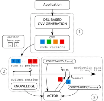
However, in practice, particularly in the context of HPC applications, GP can be very difficult to apply. Actually, implementing a single version of a large scale parallelized HPC application is a long and difficult task, thus implementing multiple versions become almost infeasible. Moreover, when considering GP, the entire development process is left to the application developer. For this reason, we propose in this paper a complete automated process to take advantage of the CVV leverage. This process is depicted in Figure 1.
The CVV automation process is composed of three differ-ent phases. The first phase is responsible for the automatic generation of code versions. To do so, we propose to use Domain Specific Languages (DSLs). Among existing solutions to ease HPC programming, Domain Specific Languages target a specific domain, in opposition to general purpose (paral-lel) languages. By explicitly knowing the targeted domain, DSLs are able to automatically generates very efficient HPC codes [1]–[4]. Most of the time, DSLs are used to generate the code that reaches the smallest execution time for a given application and a given hardware architecture. In this paper we use DSLs as a mechanism to generate multiple versions of a code instead of a single one, thus creating the set of states for the CVV leverage, represented by different squared colors in Figure 1.
The second phase of the CVV automation process is to use a given subset of production runs of an application
DSL-BASED CVV GENERATION code versions production runs through time tk tk+m KNOWLEDGE ACTOR CONSTRAINTS( )tk+m+1 1 2 3 CVV Application 1 2 ... 1 2 CONSTRAINTS( )tk+m tk+m+1 1 2 Another leverage runs to perform collect metrics 1 2
Fig. 1: Automation process of the CVV leverage
to combine leverages, thus building a knowledge, which is complete at tk. The number of runs needed to reach a complete
knowledge tk depends on the prediction degree handled in the
knowledge building process: from “Null”, where all leverages combinations has to be performed, to “High” where all of the knowledge is present from start (without the use of any previous run). One can note that the knowledge is built upon a given set of metrics.
The knowledge built in the second phase is then used within the third phase, for any new production run that happens after tk, to take decision regarding the code version to use for this
new production run according to the current constraints. The element which is responsible for this decision is called an actor. An example of actor is the OnDemand linux governor which chooses the DVFS current state depending on the current system load2
More formally, let L be the set of possible leverages, and C a set of constraints to fulfill (of any type). We also denote states(L) the function that returns the set of states S of a leverage L.
Definition 3. An actor a is a function that for a subset of leveragesLsub ⊂ L and a set of constraints C ∈ Cn returns
a set of new choosen states Sres, one for each leverage of
L ∈ Lsub.Each new states0c returned by an actora is called
a choice.
An actor aims at fulfilling constraints by choosing new states s0c ∈ states(L). When considering multiple
optimiza-tion objectives, possibly not compatible, a trade-off has to be found between all constraints and objectives of C.
III. CASE STUDY DESCRIPTION
In this section is described the case-study addressed within the paper. Regarding the automation process depicted in Figure 1, this section presents first the application use-case, second, the DSL used to generate CVV states, third, how the knowledge is built and used by actors, and finally, which constraints are handled.
A. FullSWOF2D application
As already explained, the automation process presented in the previous section targets regular production numerical simulations. A numerical simulation simulates a physical phenomenon by approximating the exact solution of partial differential equations through a set of numerical schemes (computations). A numerical simulation discretizes the time through a time loop. At each time iteration, a set of numer-ical computations are applied onto the entire (or a subset) discretized space domain (namely a mesh). A numerical sim-ulation is typically composed of (i) a number of iteration, (ii) a mesh size, (iii) a set of numerical parameters (single numerical values) and (iv) a set of input data sets representing physical quantities (e.g., speed, pressure etc.). Those physical quantities are mapped onto the mesh.
For a given domain size (i.e., mesh size), a production numerical simulation is used many times by physicists, modi-fying input data sets and numerical parameters, to be as close as needed to the real phenomenon to understand it.
A numerical simulation can be regular or irregular. In this paper regular simulations are handled. More particularly, stencil-based numerical simulations are considered. Thus, the same set of computations are performed whatever numerical values of input data sets and parameters are. As a result, by considering the same set of machines (i.e., same cluster) and the same input size, performance behavior of stencil-based codes stay the same3. This makes possible to reuse
the knowledge built within the automation process for many production runs.
As an example of production numerical simulation, we consider FullSWOF2D4 [5] (denoted FS2D), developed at
the MAPMO laboratory, University of Orl´eans, France. FS2D consists in solving the Shallow Water equations (two dimen-sional Navier-Stokes equations) using finite volumes methods especially chosen for hydrodynamic purposes (transitions be-tween wet and dry areas, small water heights, etc.). FS2D is a complex numerical simulation composed of 32 stencil kernels and 66 local kernels [6].
As an illustration, in production, FS2D will be run many times with the same input size. Actually inputs of FS2D are 8 numerical parameters (e.g., hydrolic conductivity, water viscosity, pressure etc.), and 6 input data sets (e.g., rain, speed in each dimension etc.). Each parameter and data set can be initialized in very different manners to study different physical cases (already flooded grounds, dry grounds etc.)
3http://www.agner.org/optimize/instruction tables.pdf 4http://www.univ-orleans.fr/mapmo/soft/FullSWOF/
When considering simply 2 possible values for each parameter and 2 possible input data sets, the number of possible runs is the cartesian product 28× 26= 214= 16, 384. This illustrates
that a production numerical simulation can be used many times using the same input size. FS2D will be the considered application for the rest of this paper.
B. The Multi-Stencil Language
The domain specific Multi-Stencil Language (MSL) [6] enables to automatically generate multiple HPC code versions of a multi-stencil numerical simulation from a lightweight data-oriented description of a numerical application and a set of sequential kernel codes. The semantic and performances of MSL has been shown in [6]. In this paper, MSL is used to generate four HPC code versions of FS2D, thus producing the set of states SA of the CVV leverage.
These four versions are based on two different paral-lelization techniques. The first technique, namely data par-allelization, divides the studied domain (data) into equally balanced sub-domains. Each sub-domain is computed by one computational resource (typically a core) and communications between resources are added to perform correct computations. The second technique, namely task parallelization, divides a program into sub-tasks. Each task is computed by one computational resource, and task dependencies are introduced to respect computation order. The scheduling of task de-pendencies can be statically computed before the execution, or can be dynamically decided at runtime. In MSL these techniques are implemented by using the Message Passing Interface (MPI) and the OpenMP Application Programming Interface. The four code versions produced by MSL are: (1) MpiBase, where data parallelization is applied by domain decomposition and by using MPI; (2) MpiOmpFor, where data parallelization is introduced at two different levels, first, by domain decomposition with MPI, and second, by using parallel loops of OpenMP; (3) MpiOmpForkJoin, where both data and task parallelization techniques are combined, and where the adopted task parallelization technique is a static fork/join scheduling implemented using OpenMP; and finally (4) MpiOmpDyn, where both data and task parallelization techniques are also combined, but where the adopted task parallelization technique is the dynamic scheduling of tasks introduced in OpenMP 4.55.
One can note that these four code versions represent dif-ferent approaches to parallelize the code. Many other code versions could be studied such as versions using various cache optimizations, different types of data, etc. These four versions, though, are difficult to write by hand, thus being an interesting case-study for GP automation.
C. Knowledge, actors and constraints
To entirely understand the case-study adressed within this paper, it is needed to describe how the knowledge is built and used by the automation process.
First, as depicted in Figure 1 the knowledge is built by using a certain number of production runs until tk is reached,
which means that the knowledge is complete. The number of runs to perform before reaching tk depends on the number of
possible combinations when exploring a set of leverages. In this paper are considered two different leverages. The first one is the CVV leverage described in Section II, the second one is the leverage that modifies the number of MPI processes and OpenMP threads for a given parallel application on a given subset of nodes. This last leverage has already been used in [7]–[9]. As an example, our complete knowledge (combina-tions of code versions and MPI/OpenMP configura(combina-tions) when 12 cores are available per machine (Table I of Section IV-A) contains 55 production runs. As illustrated before, a very light use of FS2D in production already leads to 16,384 runs. This shows that our technique is realistic and feasible in our case-study.
Of course, when increasing the number of leverages (i.e., the number of choices), the size of the knowledge to build also increases. For this reason, actors could be more or less intelligent and could need a smaller knowledge to take a good decision (e.g., machine learning techniques). This type of actors will be simulated during our evaluations in Section V. For each of the production runs used to build the knowledge (before tk), four metrics are collected. The first metric is
the Execution Time, denoted time. It measures the entire execution time of one job, including initialization time. The three remaining metrics are energy-related metrics. To define these metrics, we first need to introduce some notations:
• N is the number of computing nodes used by a job; • T = {t0, . . . , tn−1} is the set of n time stamps of energy
consumption measurements of a job; t0and tn represent
the starting and ending timestamps, respectively;
• pi
j, where i ∈ [0, N − 1], and j ∈ [0, n − 1], represents
the power consumption (in Watt), of a node i for the timestamp tj;
• Pj = Pi∈[0,N −1]p i
j represents the cumulated power
measurements of all nodes i ∈ [0, N − 1] for a given timestamp tj ∈ [0, n − 1].
The second metric is the Maximum Cumulated Watt and is denoted maxCW att. It represents the cumulated maximum power witnessed during the run of the application A for the set of current selected states sc of considered leverages.
It reflects how much the application, when considering the current combination of leverage states, stresses the computing nodes on which it is executed. It is defined as:
maxCW att = max
j∈[0,n−1]
Pj (1)
The third metric is the Average Cumulated Watt and is denoted avrgCW att. It represents the cumulated average power consumption of the application A for the set of current states. It is defined as follows:
avrgCW att = P
j∈[0,n−1]Pj
n (2)
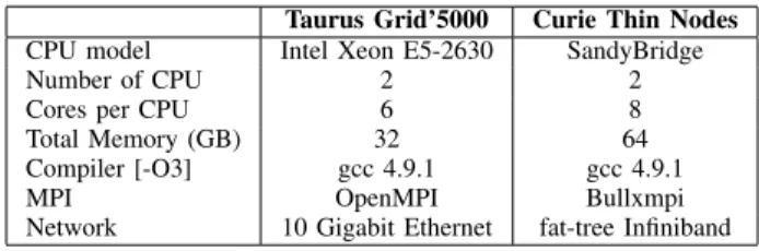
TABLE I: Hardware configuration of Grid’5000 Taurus nodes and TGCC Curie thin nodes
Taurus Grid’5000 Curie Thin Nodes CPU model Intel Xeon E5-2630 SandyBridge Number of CPU 2 2 Cores per CPU 6 8 Total Memory (GB) 32 64 Compiler [-O3] gcc 4.9.1 gcc 4.9.1 MPI OpenMPI Bullxmpi Network 10 Gigabit Ethernet fat-tree Infiniband
Finally, the fourth metric is the Cumulated Joules and is denoted CJ oules. It represents the cumulated energy con-sumption of the run for the current leverages combination. It is the energy consumption of all nodes used between t0and
tn for the execution of A. It is defined as follows:
CJ oules = X
j∈[0,n−1]
(tj+1− tj) ∗ Pj (3)
In the rest of this paper we consider a single constraint, the power capping. A power capping constraint indicates a maximum power consumption value to not overpass during a certain period of time. This is the type of constraints imposed by electrical providers within their contracts or through a scheduler imposing various power capping to every user [10].One can note that this constraint can evolve through time. In addition to this constraint, two functions have to be minimizes: the execution time of each run; and the energy consumption of each run.
In this section has been presented our complete considered case-study. This case-study illustrates that our automation process of Green Programming is feasible. In the rest of this paper are detailed the experiments conducted on this case-study.
IV. EXPERIMENTAL SETUP
In this section is detailed the experimental setup used for evaluations. First, the hardware is described, then the chosen configurations to build knowledges are given.
A. Hardware and energy monitoring
To conduct our evaluation, we use the Grid’5000 experi-mental platform and the Curie supercomputer. Grid’50006 is a
French large-scale and versatile testbed for experiment-driven research in all areas of distributed computing. Experiments presented in this paper have been conducted on the cluster named Taurus of the site of Lyon. The hardware configuration of this cluster is given in Table I. Each node is monitored by a wattmetter with a precision of 0.125 Watt (W) and that reports the average of 3600 measurements each second.
The TGCC Curie7 is a French petascale supercomputer
ranked as the 93th supercomputer of the Top500 list of November 20178. It is composed of three different types of
6http://www.grid5000.fr
7http://www-hpc.cea.fr/fr/complexe/tgcc-curie.htm 8http://www.top500.org/lists/2017/11/
TABLE II: Knowledge configurations on FS2D.
Knowledge Cluster #nodes Domain size #Iteration A Taurus G5k 4 4000 × 4000 100 B Thin Curie 128 20000 × 20000 10000
nodes, each with a specific hardware configuration. Experi-ments of this paper have been performed on the Thin Nodes (Table I) of the TGCC Curie supercomputer. Measurements on Curie thin nodes are done at the electrical cabinet with dedicated wattmeters and are updated approximately every 5 minutes.
B. Knowledge configurations and representation
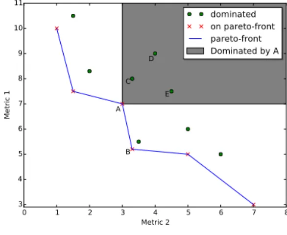
By using code versions (CVV) generated by MSL on FS2D for Phase 1 of Figure 1, we run a set of benchmarks to build Knowledges. A Knowledge is built upon application produc-tion runs that combine leverages for a given configuraproduc-tion (domain size and number of iterations). Moreover, each run collects a set of metrics, as detailed in Sections II-B and III-C. Two Knowledges have been built in our evaluations and are summarized in Table II for Grid’5000 and Curie experiments. To analyze multiple metrics at the same time, we have chosen to use a pareto representation and its associated pareto frontier (or pareto-front) formally defined for energy concerns in [9]. Figure 2 gives an example of a 2D pareto frontier, where each axis is a metric and each point represents measures registered for a given job of a benchmark campaign.
0 1 2 3 4 5 6 7 8 Metric 2 3 4 5 6 7 8 9 10 11 Metric 1 A B C D E dominated on pareto-front pareto-front Dominated by A
Fig. 2: Pareto frontier example
Points on the pareto frontier represent the set of best solutions (relative to the remaining points), for a trade off between the two chosen metrics. Thus, they represent choices where no improvement for a metric can be made without deteriorating the second one. Points on the pareto-front are called dominant points while others are called dominated points. For example, in Figure 2, where both metrics have to be minimized, choosing B over A decreases the first metric but increases the second one. Points C, D, and E are dominated by A, which means that both metrics increase compared to A. There is a wide panel of possible trade-offs between two chosen metrics. The trade-off could be between two energy
metrics or between an energy metric and the execution time. Our benchmark framework executes a set of jobs which are the combination of two application leverages. First, the set of available code versions of FS2D (CVV), and second, the MPI/OpenMP configuration chosen to run FS2D. From the results produced by one campaign, a pareto can be built, where each point represents one job. To build a pareto, two metrics among the described ones in Section III-C have to be chosen.
V. CASE STUDY EVALUATION
This section presents the evaluations of, first, the CVV leverage alone, second, the CVV leverage combined to the MPI/OpenMP leverage. Finally, we present through simulation two complete production scenario evaluations.
A. Evaluation of the CVV leverage
First, we would like to show in our evaluations that choosing one code version or another while mesuring time, maxCWatt, avrgCWatt and CJoules, leads to a non trivial tradeoff. Table III reports measurements of the four metrics when executing the same knowledge configuration A, with the four code versions generated by MSL, on a single Taurus node. The Taurus node is used with its full capacity, thus using its 12 cores.
From Table III, we can obserse that “MpiOmpFor” and “MpiOmpForkJoin” are minimizing time and CJoules, respec-tively. However, these code versions also have the highest values for maxCWatt and avrgCWatt. As a result, and as expected, a correlation exists between the execution time and the energy consumption (CJoules). However, minimizing these metrics leads to high power consumption that could be problematic in the case of power capping constraints either for a cluster administrators or a green scheduler translating energy budget to a power capping. Moreover, Table III shows that for every state of the CVV leverage (code version), non negligible variability can be observed in the four metrics. B. Combination of CVV and MPI/OpenMP leverages
When combining the CVV leverage with the leverage that configures the number of MPI processes and the number of OpenMP threads, the number of possible choices to get the best trade-off between metrics increases, thus the choice can be improved. Both Figures 3a and 3b illustrate this claim.
In Figure 3a, Knowledge A is built with four nodes of the Taurus cluster of Grid’5000. Each symbol (or color) refered to one code version among the four code versions generated by MSL on FS2D. For each code version, many
TABLE III: Time, maxCWatt, avrgCWatt and CJoules for the four different code versions generated by MSL on FS2D (CVV).
time(s) maxCWatt avrgCWatt CJoules MpiOmpDyn 133.37 253.25 237.97 31916.5 MpiOmpFor 128.25 257.87 239.80 30854.12 MpiOmpForkJoin 130.75 257.0 239.29 31515.25 MpiBase 142.5 254.87 235.22 33733.87
different configurations of MPI/OpenMP are possible, each point for one symbol (or color) represents one configuration. For example, the code version MpiOmpForkJoin can be run be using 4 MPI processes and 12 OpenMP threads per MPI process, or can be run by using 8 MPI processes and 6 OpenMP threads per MPI process. In this case cores of the four nodes are fully used (12 per node), but the same benchmark can be executed by using only 4 MPI processes and 2 OpenMP threads, etc.
Figure 3a presents a pareto on the metrics time and avrgCWatt, where all runs of the knowledge A are represented (55 different runs). Each run has been performed 8 times and a median is computed. The pareto frontier is represented in blue. One can note a variability of code versions on the pareto frontier. This means that among the set of best choices for a trade-off between time and avrgCWatt, multiple code versions are represented. As a result, the CVV leverage improves the trade-off that MPI/OpenMP leverage alone could reach.
For example, in Figure 3a, if we consider a power capping constraint set to 600W , the chosen state for the CVV leverage would be “MpiOmpDyn” (associated to a given MPI/OpenMP configuration). In fact, it is the first point on the pareto-front to answer the fixed constraint. Thus by definition, it is the point that minimizes execution time while satisfying this power capping constraint.
One can note that the same result can be observed on Curie regarding the knowledge B in Figure 3b. Because of our limited access to thin nodes of TGCC Curie, one can note that less jobs have been performed than on Grid’5000 resulting in less points onto the pareto, thus an incomplete knowledge. However, the same conclusions can be taken as the results show that different code versions are represented on the pareto frontier. As a conclusion, the CVV leverage is also interesting at large scale.
C. Simulation of Production Scenarios
To have a complete control over the applied scenarios, we have chosen to simulate different production and power constraints scenarios.
The knowledge presented in Figure 3a is used within our simulation. Three different elements are simulated within a given scenario: (1) the production scenario; (2) the energy and power constraints considered during the production scenario; and (3) the set of actors considered.
1) Production scenarios: The first production scenario is called soft. A total number of 210= 1, 024 runs are performed within this entire production scenario which is much less than the example given throughout this paper (16, 384 production runs). Thus, this scenario is not in favor of our process. This production scenario has a low frequency usage with four runs a day (two of them during the night, and two of them during the daytime). This scenario represents a soft arrival of production runs during 256 days.
In the second production scenario, namely hard, the same total number of runs are performed. However a high arrival frequency is simulated. Actually, twenty runs are performed
per day which leads to a hard use of production resources for 52 days (51 full days, plus 4 extra runs during 52th day). To make these scenarios more realistic we also introduce vacan-cies or maintenance periods where runs are not performed.
2) Constraints: For the power constraints, we have chosen to simulate two types of power capping constraints. On one hand, the first constraint, namely Fixed, represents a power capping value (i.e., maximum value to not overpass) constant through time. To choose a real case power capping for knowl-edge A, we refer to results displayed in Figure 3a, where we have chosen the rounded value equidistant to the minimum and maximum reached avrgCWatt on the pareto-front. Thus, 650W has been chosen as Fixed constraint.
The second power constraint is denoted day-night. In this constraint, the maximum power value is low during daytime and high during night. For knowledge A, 600W and 800W have been chosen for day and night power constraint, respec-tively.
3) Actors: The two first actors considered in our simulation do not base their choice on any knowledge. The first actor of this family is called Usual. This actor illustrates what usually happens in production, i.e., a single code version and a single MPI/OpenMP configuration are used for all runs. The second one is denoted Random. This actor randomly chooses one code version and one MPI/OpenMP configuration for each production run. One can note that both Usual and Random can perform choices that do not respect input constraints. However, the power capping constraints has been chosen such that Usual never violate it. One can note that this choice is not in favor of our process once again.
The third actor is the one we advocate in this paper. It is called BuildKlg. This actor makes choices by using a full knowledge (i.e., complete paretos).
The last considered actor is called Ideal. This actor uses advanced machine learning strategies to be able to make choices with a partial knowledge of previous runs. Thus, this actor reduces the number of runs needed to reach tk. As this
paper does not focus on the proposal of new actors, we have made the hypothesis that this Ideal actor is able to accurately discover the complete knowledge without any previous run, which would be the perfect actor, even if not feasible. Thus this actor represents the theoretical best case of our simulation. Both BuildKlg and Ideal aims at first respecting power capping constraints and second minimizing execution time and energy consumption.
4) Simulation results: This section analyses the results of simulation for every proposed actor on any production scenario and for any considered power constraint.
Two metrics are considered in results. First, the Violation metric represents the amount of joules consumed over the fixed power limit (the bigger the value, the worst the actor is). We could imagine that every joules consumed over the limit represent an extra cost. This metric is relevant to a user that estimates that power capping must not be exceeded, during all run. However, as the input cost per joule highly depends on the infrastructure or electrical provider policies, we represents
0 50 100 150 200 250 300 350 time (s) 500 600 700 800 900 avrgCWatt (W) mpiOmpFor mpiBase mpiOmpDyn mpiOmpForkJoin
(a) Pareto representing the knowledge A by using 4 Taurus nodes of Grid’5000 1500 2000 2500 3000 3500 4000 4500 time (s) 20000 25000 30000 35000 40000 avrgCWatt (W) mpiOmpFor mpiBase mpiOmpDyn mpiOmpForkJoin
(b) Pareto representing the knowledge B by using 2048 cores (or 128 Thin nodes) of Curie
Fig. 3: Paretos with metrics time and avrgCW att, for knowledges A and B of Table II.
TABLE IV: Simulation results based on knowledge A in terms of energy consumption, violation of constraints, and associated percentages compared to the Usual actor.
Actor Energy (J) Violation(J) % gain % Violation Soft, Fixed Usual 54192768,00 0,00 0,00 0,00 Ideal 31659648,00 0,00 41,58 0,00 Random 55849891,19 7465509,76 -3,06 13,37 BuildKlg 32619458,62 133449,82 39,81 0,41 Soft, Day-night Usual 54192768,00 0,00 0,00 0,00 Ideal 43075597,13 1440879,81 20,51 3,35 Random 55867662,19 7074282,00 -3,09 12,66 BuildKlg 43567042,87 1686303,71 19,61 3,87 Hard, Fixed Usual 54192768,00 0,00 0,00 0,00 Ideal 31659648,00 0,00 41,58 0,00 Random 55179811,31 3242795,56 -1,82 5,88 BuildKlg 32619458,62 133449,81 39,81 0,41 Hard, Day-night Usual 54192768,00 0,00 0,00 0,00 Ideal 47837186,63 288175,96 11,73 0,60 Random 55849891,19 7465509,76 -3,06 13,37 BuildKlg 48165244,49 573153,42 11,12 1,19
the percentage of violation metric rather than the cost. Second, the total energy consumption is represented.
Table IV displays the results of these simulations. The total energy consumed and the violation of constraints are represented for every scenario. Percentage of saved energy, and constraint violation are given using the Usual actor as a refer-ence. Actually, for the Usual actor, the CVV leverage position is set to mpiOmpDyn. While the MPI/OpenMP leverage is set to 4/10 (4 MPI processes and 10 threads per MPI process). Moreover, we have chosen this configuration because it always answers power capping constraints. Thus the simulated overall consumption of Usual actor will always be the same, given that the chosen run is always the same.
Regarding the violation rate, Random is the worst actor. One can note that BuildKlg has very low percentage of violation
(3.88% in the worst case, 0.41% in the best case). Moreover, BuildKlg is very close to Ideal which is the best possible actor for this metric. The differences between these two is the discovery part. In fact, during the pareto construction (dis-covering all the CVV and MPI/OpenMP states combinations) the BuildKlg actor violates the constraints. Even Ideal has penalties on Day-Night senario. This is due to the fact that we only consider knowledge of constraints at the start of a run. Thus, such penalties are due to a change of the constraint value during the run (e.g., for job starting the night and finishing during the day).
If we only focus on the percentage of gain compared to Usual, the tendencies are the same for every scenario. Random is always worst than Usual (negative percentage of gain), showing that the state of both the CVV and the MPI/OpenMP leverages is not something to choose randomly. For BuildKlg, we can see that for each case, energy savings are not negligible (around 11% in the worst case, and up to 39% in the best case). Ideal reaches the best energy savings but is very close to BuildKlg (a difference of 1.77% in the worst case), implying that such a clever actor may not be needed, in our case study. In our evaluations we have shown that our automated process of Green Programming is applicable on a real case-study, and can almost reach ideal results for both the total energy consumption and the rate of power capping violations. Thus, this work leads to energy and money savings.
VI. RELATED WORK ON APPLICATION LEVERAGES
Many works have dealt with the configuration variation of a given application to get an energy-aware usage of computing nodes. In [9], authors provide a mathematical formulation of the multi-objective performance tuning problem. The work shows that energy-aware configurations of application are possible. The number of MPI processes and the number of OpenMP threads are again both used as leverages.
In [11], authors present a predictive model to estimate power consumption and computation performances (i.e., execution
time). The prediction is made for a given device. A single version of code is given for each device from CPU to GPU. Thus, in this work, the selected version of code is actually used to choose the best type of hardware to save energy. In [9], authors explore the variability of the energy consump-tion of multiple CPU while using DVFS. Code versions are provided as different binaries of the same application. Thus, the work points out the possibility of obtaining multiple energy consumption behaviours by selecting a version of code while varying the frequency of the processor.
In [12] authors use an auto-tuning framework to study different code versions under energy concerns. Thus, this work is close to our contribution. Actually, our automation process could be compared to an auto-tuning solution. However, a first difference is that the above work is limited to the first phase of our automation process, not considering production scenarios and knowledge construction time. Second, the auto-tuning framework used in the work generates different loop transformation strategies while we study different parallel code versions of a production numerical simulation. Finally, our contribution also combines two different application level leverages to enhance possible choices.
As a sum-up, previous related works have shown that the configuration of the number of OpenMP threads and (or) the number of MPI processes help controling the energy consumption of nodes. Several other recent works have studied code variability as a possible leverage. However, none of the previous papers have contributed to an automation process of the CVV usage, and none of them have defined and used the CVV leverage as presented in this paper. Moreover, none of these works have studied the feasability of such Green Programming (GP) concept for production HPC numerical simulations. Finally, none of the previous papers have explored an evaluation of two application level leverages (configuration and version of code leverages) in the same experiment, which enhance energy choices.
VII. CONCLUSION
In this paper, four contributions have been presented toward automated Green Programming in HPC context. First, we have introduced a formal definition of the Code Version Variability (CVV) leverage. During evaluation, we have underlined that the usage of the CVV leverage alone, as well as combined with another leverage, offers more variability of choices, thus better trade-offs between execution time, energy consumption and power metrics.
Second, we have presented and detailed a first approach toward Green Programming (GP) automation in the specific case of production applications that are regulars.
Third, our automation process of GP has been applied to a real case-study where a real-case numerical simulation has been selected, where a real-case DSL [6] has been used to produce different code versions, and where r constraints have been considered. This case-study have shown the feasibility of our automation.
Finally, we have shown in our evaluations that our auto-mated GP, applied onto our case-study, gets significant energy savings as well as very low constraints violations. compared to a usual production case (no leverages considered), compared to a random case (by
Future work includes the integration of such an automation within middleware level leverages such as a schedulers. We also plan to combine our approach with hardware leverages like DVFS or Shutdown techniques. Finally, we would like to consider reconfiguration of code versions at runtime.
REFERENCES
[1] Z. DeVito, N. Joubert, F. Palacios, S. Oakley, M. Medina, M. Barrientos, E. Elsen, F. Ham, A. Aiken, K. Duraisamy, E. Darve, J. Alonso, and P. Hanrahan, “Liszt: A domain specific language for building portable mesh-based pde solvers,” in Proceedings of 2011 International Conference for High Performance Computing, Networking, Storage and Analysis, ser. SC ’11. New York, NY, USA: ACM, 2011, pp. 9:1–9:12. [Online]. Available: http://doi.acm.org/10.1145/2063384.2063396 [2] C. Schmitt, S. Kuckuk, F. Hannig, H. K¨ostler, and J. Teich,
“Exaslang: A domain-specific language for highly scalable multigrid solvers,” in Proceedings of the Fourth International Workshop on Domain-Specific Languages and High-Level Frameworks for High Performance Computing, ser. WOLFHPC ’14. Piscataway, NJ, USA: IEEE Press, 2014, pp. 42–51. [Online]. Available: http://dx.doi.org/10.1109/WOLFHPC.2014.11
[3] J. Ragan-Kelley, C. Barnes, A. Adams, S. Paris, F. Durand, and S. Amarasinghe, “Halide: A language and compiler for optimizing parallelism, locality, and recomputation in image processing pipelines,” in Proceedings of the 34th ACM SIGPLAN Conference on Programming Language Design and Implementation, ser. PLDI ’13. New York, NY, USA: ACM, 2013, pp. 519–530. [Online]. Available: http://doi.acm.org/10.1145/2491956.2462176
[4] Y. Tang, R. Chowdhury, B. Kuszmaul, C.-K. Luk, and C. Leiserson, “The pochoir stencil compiler.” in SPAA, L. Fortnow and S. P. Vadhan, Eds. ACM, 2011, pp. 117–128. [Online]. Available: http://dblp.uni-trier.de/db/conf/spaa/spaa2011.html#TangCKLL11 [5] H. Coullon and S. Limet, “The SIPSim implicit parallelism model
and the SkelGIS library,” Concurrency and Computation: Practice and Experience, 2015. [Online]. Available: https://hal.archives-ouvertes.fr/ hal-01149418
[6] H. Coullon, J. Bigot, and C. Perez, “Extensibility and composability of a multi-stencil domain specific framework,” International Journal of Parallel Programming, Nov 2017. [Online]. Available: https: //doi.org/10.1007/s10766-017-0539-5
[7] D. Li, B. R. de Supinski, M. Schulz, K. W. Cameron, and D. S. Nikolopoulos, “Hybrid mpi/openmp power-aware computing.” in IPDPS, vol. 10, 2010, pp. 1–12.
[8] A. Marathe, P. E. Bailey, D. K. Lowenthal, B. Rountree, M. Schulz, and B. R. de Supinski, “A run-time system for power-constrained hpc applications,” in International Conference on High Performance Computing. Springer, 2015, pp. 394–408.
[9] P. Balaprakash, A. Tiwari, and S. M. Wild, “Multi objective optimization of hpc kernels for performance, power, and energy,” in International Workshop on Performance Modeling, Benchmarking and Simulation of High Performance Computer Systems. Springer, 2013, pp. 239–260. [10] Y. Georgiou, D. Glesser, K. Rzadca, and D. Trystram, “A scheduler-level
incentive mechanism for energy efficiency in hpc,” in Cluster, Cloud and Grid Computing (CCGrid), 2015 15th IEEE/ACM International Symposium on. IEEE, 2015, pp. 617–626.
[11] P. E. Bailey, D. K. Lowenthal, V. Ravi, B. Rountree, M. Schulz, and B. R. De Supinski, “Adaptive configuration selection for power-constrained heterogeneous systems,” in 2014 43rd International Conference on Parallel Processing. IEEE, 2014, pp. 371–380.
[12] A. Tiwari, M. A. Laurenzano, L. Carrington, and A. Snavely, Auto-tuning for Energy Usage in Scientific Applications. Berlin, Heidelberg: Springer Berlin Heidelberg, 2012, pp. 178–187. [Online]. Available: https://doi.org/10.1007/978-3-642-29740-3 21