Improving IoT data stream analytics using summarization techniques

(1)

HAL Id: tel-02865982

https://tel.archives-ouvertes.fr/tel-02865982

Submitted on 12 Jun 2020

HAL is a multi-disciplinary open access archive for the deposit and dissemination of sci-entific research documents, whether they are pub-lished or not. The documents may come from teaching and research institutions in France or abroad, or from public or private research centers.

L’archive ouverte pluridisciplinaire HAL, est destinée au dépôt et à la diffusion de documents scientifiques de niveau recherche, publiés ou non, émanant des établissements d’enseignement et de recherche français ou étrangers, des laboratoires publics ou privés.

summarization techniques

Maroua Bahri

To cite this version:

Maroua Bahri. Improving IoT data stream analytics using summarization techniques. Machine Learn-ing [cs.LG]. Institut Polytechnique de Paris, 2020. English. �NNT : 2020IPPAT017�. �tel-02865982�

(2)

626

NNT

:2020IPP

A

T017

Improving IoT Data Stream Analytics

Using Summarization Techniques

Thèse de doctorat de l’Institut Polytechnique de Paris préparée à Télécom Paris École doctorale n◦_{626 Dénomination (Sigle)}

Sp´ecialit´e de doctorat : Informatique

Thèse présentée et soutenue à Palaiseau, le 5 juin 2020, par

M

AROUA

B

AHRI

Composition du Jury :

Albert Bifet

Professor, Télécom Paris Co-directeur de thèse

Silviu Maniu

Associate Professor, Université Paris-Sud Co-directeur de thèse João Gama

Professor, University of Porto Pr´esident

C´edric Gouy-Pailler

Engineer-Researcher, CEA-LIST Examinateur

Ons Jelassi

Researcher, T´el´ecom Paris Examinateur

Moamar Sayed-Mouchaweh

Professor, Ecole Nationale Sup´erieure des Mines de Douai Rapporteur Mauro Sozio

Associate Professor, T´el´ecom Paris Examinateur Maguelonne Teisseire

(3)

Using Summarization Techniques

Maroua Bahri

A thesis submitted in fulfillment of the requirements for the degree of

Doctor of Philosophy

Télécom Paris

Institut Polytechnique de Paris

Supervisors:

Albert Bifet

Silviu Maniu

Examiners:

João Gama

Cédric Gouy-Pailler

Ons Jelassi

Moamar Sayed-Mouchaweh

Mauro Sozio

Maguelonne Teisseire

Paris, 2020

(4)

Abstract

With the evolution of technology, the use of smart Internet-of-Things (IoT) devices, sensors, and social networks result in an overwhelming volume of IoT data streams, generated daily from several applications, that can be transformed into valuable information through machine learning tasks. In practice, multiple critical issues arise in order to extract useful knowledge from these evolving data streams, mainly that the stream needs to be efficiently handled and processed. In this context, this thesis aims to improve the performance (in terms of memory and time) of existing data mining algorithms on streams. We focus on the classification task in the streaming framework. The task is challenging on streams, principally due to the high – and increasing – data dimensionality, in addition to the potentially infinite amount of data. The two aspects make the classification task harder.

The first part of the thesis surveys the current state-of-the-art of the classification and dimensionality reduction techniques as applied to the stream setting, by providing an updated view of the most recent works in this vibrant area.

In the second part, we detail our contributions to the field of classification in streams, by developing novel approaches based on summarization techniques aiming to reduce the computational resource of existing classifiers with no – or minor – loss of classification accuracy. To address high-dimensional data streams and make classifiers efficient, we incorporate an internal preprocessing step that consists in reducing the dimensionality of input data incrementally before feeding them to the learning stage. We present several approaches applied to several classifications tasks: Naive Bayes which is enhanced with sketches and hashing trick, k-NN by using compressed sensing and UMAP, and also integrate them in ensemble methods.

(5)

(6)

I dedicate to my sweet loving

Father, Mother & Siblings

whose unconditional love, encouragement, affection, and

prays of day and night make me able to get such success

and honor. Without them, I would never get through this.

(7)

(8)

List of Figures

1.1 IoT connected devices. . . 6

1.2 The thesis context. . . 9

1.3 Contributions of the thesis. . . 10

2.1 Sliding window model. . . 18

2.2 Landmark window of size 13. . . 18

2.3 Damped window model. . . 19

2.4 The data stream classification cycle. . . 21

2.5 Taxonomy of classification algorithms. . . 22

2.6 Ensemble classifier. . . 24

2.7 Taxonomy of dimensionality reduction techniques. . . 25

2.8 Handling data stream constraints. . . 33

3.1 Count-min sketch. . . 41

3.2 Hashing trick. . . 49

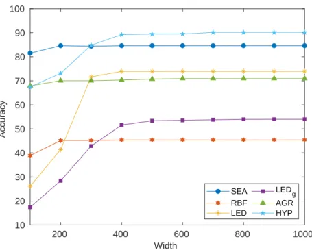
3.3 Classification accuracy with different sketch sizes. . . 52

3.4 Sorted plots of accuracy, memory and time over different output dimensions 55 4.1 Compressed kNN Scheme. . . . 63

4.2 Sorted plots of accuracy, time and memory over different output dimensions. 72 5.1 CS-ARF and ARF comparison. . . 81

5.2 Accuracy comparison over different output dimensions on Tweet1 dataset. . 83

5.3 The standard deviation of the methods while projecting into different dimen-sions . . . 84

5.4 Memory comparison of the ensemble-based methods on all the datasets. . . 85

6.1 Projection of CNAE dataset in 2-dimensional space. . . 91

6.2 Stream of mini-batches. . . 92

6.3 Batch-incremental UMAP-kNN scheme. . . . 93

(13)

6.5 Comparison of UMAP-kNN, tSNE-kNN, PCA-kNN, and kNN (with the entire

datasets) while projecting into 3 dimensions. . . 97

6.6 Comparison of UMAP-kNN, PCA-kNN, UMAP-SkNN, and UMAP-HAT over different output dimensions using Tweet1. . . 100

A.1 MOA main window. . . 110

A.2 SketchNB classifier. . . 111

A.3 Hashing trick filter. . . 111

A.4 CS-kNN algorithm. . . . 112

(14)

List of Tables

1.1 Comparison between static and stream data. . . 8

2.1 Window models comparison. . . 19

3.1 Overview of the datasets. . . 51

3.2 Accuracy comparison of SNB, GMS, NB, kNN, ASNB, AdNB, and HAT. . . . . 53

3.3 Memory comparison of SNB, GMS, NB, kNN, ASNB, AdNB, and HAT. . . . . 54

3.4 Time comparison of SNB, GMS, NB, kNN, ASNB, AdNB, and HAT. . . . 54

3.5 Accuracy comparison of SNBHT, GMSHT, NBHT, kNNHT, ASNBHT, AdNBHT, and HATHT. . . 56

3.6 Memory comparison of SNBHT, GMSHT, NBHT, kNNHT, ASNBHT, AdNBHT, and HATHT. . . 56

3.7 Time comparison of SNBHT, GMSHT, NBHT, kNNHT, ASNBHT, AdNBHT, and HATHT. . . 56

4.1 Accuracy comparison of CS with Bernoulli, Gaussian, Fourier matrices, and the entire dataset. . . 64

4.3 Performance of kNN with different window sizes. . . . 69

4.4 Accuracy comparison of CS-kNN, CS-samkNN, HT-kNN, PCA-kNN, and kNN over the whole dataset. . . 70

4.5 Time comparison of CS-kNN, CS-samkNN, HT-kNN, PCA-kNN, and kNN over the whole dataset. . . 70

4.6 Memory comparison of CS-kNN, CS-samkNN, HT-kNN, PCA-kNN, and kNN over the whole dataset. . . 71

4.7 Accuracy comparison of CS-kNNLB_{, CSB-kNN, CS-HTree}LB_{, and CS-ARF. .} ₇₂

4.8 Time comparison of CS-kNNLB, CSB-kNN, CS-HTreeLB, and CS-ARF. . . 73

4.9 Memory comparison of CS-kNNLB_{, CSB-kNN, CS-HTree}LB_{, and CS-ARF. . .} ₇₃

(15)

6.2 Comparison of UMAP-kNN , PCA-kNN, UMAP-SkNN, and UMAP-HAT. . . . 99

(16)

List of Abbreviations

ARF Adaptive Random Forest ADWIN ADaptive WINdowing CS Compressed Sensing CMS Count-Min Sketch

DR Dimensionality Reduction HT Hashing Trick

HAT Hoeffding Adaptive Tree IoT Internet of Things JL Johnson-Lindenstrauss

kNN k-Nearest Neighbors

NB Naive Bayes

RP Random Projection

(17)

(18)

List of Symbols

S Stream

Xi Instance, observation or data point, i from S xj_i Value of the attribute j of instance i

a Number of input attributes

m Number of output attributes after reduction R Set of real numbers

Ra Set of a-dimensional real vectors Rm Set of m-dimensional real vectors Rm×a Set of m × a real matrices

C Set of class labels

W Sliding window

d Sketch depth

w Sketch width

(19)

(20)

Part I

(21)

(22)

Data stream learning is a hot research topic in Machine Learning and Data Mining, that has motivated the development of several very efficient algorithms in the streaming setting. Our thesis deals with the elaboration of new classification approaches based on well-known summarization techniques. These proposed approaches make it possible to learn from – and make predictions on – evolving data streams using small computational resources while keeping good classification performance.

This part presents the necessary background concerning our thesis and is composed of two chapters:

• Chapter1provides an overview of the context and motivation of the thesis, followed by our principal contributions.

• Chapter2gives the necessary background regarding the streaming framework, its challenges and limitations. We cover the definition of the basic concepts of the stream context, such as the processing and summarization techniques for data streams. In this chapter, we also review the state-of-the-art of streaming classification and dimensionality reduction that are relevant to this thesis.

(23)

(24)

1

Introduction

Contents

1.1 Context and Motivation . . . . 5

1.2 Challenges . . . . 7

1.3 Contributions . . . . 9

1.4 Publications . . . . 12

1.5 Outline . . . . 13

1.1 Context and Motivation

Artificial Intelligence (AI) is defined as field of study in Computer Science that aims to

produce smart machines capable to mimic natural intelligence displayed by humans. The last few decades have witnessed a tremendous pace in the pervasiveness of technology that invades our world in all dimensions and keeps skyrocketing. This evolution includes, more and more, systems and applications that continuously generate vast amounts of data in an open-ended way as streams.

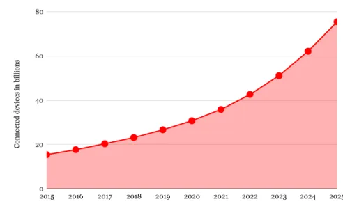
This incredibly huge quantity of data, derived daily from applications in AI, includes areas such as robotics, natural language processing, and sensor analytics [1]. As an instance application, the Internet of Things (IoT) is defined as a large network of physical devices and sensors (objects) that connect, interact, and exchange data. IoT is a key component of life automation, e.g., cars, drones, airplanes, and home automation. These devices will be creating a massive quantity of big data, via real-time streams, in the near future. By the end of 2020, 31 billion of such devices will be connected, and by 2025 this number is

(25)

Connected devices in billions 0 20 40 60 80 2015 2016 2017 2018 2019 2020 2021 2022 2023 2024 2025

Figure 1.1: IoT connected devices from 2015 to 2025.

expected to grow, according to Statista1, to around 75 billion of these devices that will be in use around the world, see Figure1.1. Hence, methods and applications must be explored to cope with this tremendous flow of data that exhibit the so-called “3 Vs”, volume, velocity, and variability.

There exist different ways to treat, organize and analyze this fast generated data using algorithms and tools from AI and data mining. Indeed, these techniques are often carried out by automated methods such as the ones from machine learning. The latter is a fundamental subset of AI that is based on the assumption that computer algorithms can learn from new data and automatically improve themselves without – or with minimal – external intervention (human intervention in general). Machine learning algorithms are characterized by learning from observations and then, make predictions using these observations in order to build appropriate models [2].

The success of IoT has motivated the field of data mining which consists in being able to extract useful knowledge by automatically acquiring the hidden insights, non-trivial, in the vast and growing sea of data made available along time. Data mining is a sub-field of machine learning which includes tasks such as classification, regression, and clustering that have been thoroughly studied over the last decades. However, traditional approaches for static datasets have some limitations when applied on dynamic data streams, hence, new approaches with novel mining techniques are necessary. In this context of IoT, mining algorithms should be able to handle the infinite and high-velocity of IoT data streams, under finite resources – in terms of time and space. More details on these challenges are provided in Section1.2.

(26)

1.2 Challenges

To convert these data into useful knowledge, we usually use machine learning algorithms adapted for streaming data tasks, consisting of a data analysis process [3,4]. In this context, the data stream mining area has become indispensable and ubiquitous in many real-world applications. Often this category of applications generates data from evolving distributions and requires real-time – or near real-time – processing.

In the data mining field, classification is one of the most popular tasks that attempts to predict the category of unlabeled – and unseen – observations by building a model based on the attribute contents of the available data. The stream classification task is considered as an active area of research in the data stream mining field, where the focus is to develop new – or improve existing – algorithms [5]. There is a number of classifiers that are widely used in data mining and applied in several real-world applications, such as decision trees, neural networks, k-nearest neighbors, Bayesian networks, etc. The next chapter covers, inter alia, a survey on the well-known and recent classification algorithms for evolving data streams.

1.2 Challenges

As mentioned above, stream classification task aims to predict labels – or classes – of new incoming unlabeled instances from the stream while updating continuously, after prediction, the models as the stream evolves to follow the current distribution of the data. The online and potentially infinite nature of data streams, which raises some critical issues and makes traditional mining algorithms fail, imposes high resource requirements to handle the dynamic behavior of evolving distributions.

While many of the following issues are common across different data stream mining applications, we address these issues in the context of incremental classification [6,7,8].

• Evolving nature of data streams. Any classification algorithm has to take into account the considerable evolution of data and adapt to the high speed nature, because streams often deliver observations very rapidly. Thus, algorithms must incrementally classify recent instances.

• Processing time. A real-time algorithm should process the incoming instances as fast as possible because the slower it is the less efficient it will be for applications that require rapid processing.

• Unbounded memory. Due to the huge amounts and high speed of streaming data that require an unlimited memory, any classification algorithm should have the ability to work within memory constraint by maintaining as little as possible information about processed instances and the current model(s).

• High-dimensional data streams. Data streams may be high-dimensional, such as those containing text documents. For such kinds of data, distances between instances grow very fast which can potentially impact any classifier’s performance.

(27)

Table 1.1: Comparison between static and stream data.

Static data Stream data

Access random sequential

Number of passes multiple pass single pass

Processing time unbounded restricted

Memory usage unbounded restricted

Type of result accurate approximate

Environment static dynamic (evolving)

• Concept drift. One crucial issue when dealing with a very large stream is the fact that the underlying distribution of the data can change at any moment, a phenomenon known as concept drift. We direct the reader to [9] for a survey of this concept. The drift can change the classifier results over time. To cope with the new trends of data that must be detected at the same time as their appearance, a drift detection mechanism is usually coupled with learning algorithms.

In the stream setting, a crucial question arises about how to process infinite data over time while addressing the stream framework requirements with minimal costs?

These above-mentioned challenges are of special significance in the stream classifica-tion. We notice that stream mining techniques must differ from the traditional ones for static datasets. To handle these challenges, classification algorithms must incorporate an incremental strategy that permits such processing requirements presented in Section2.2. Table1.1presents a comparison of environments for both static and stream data [10].

In addition to the overwhelming volume of data, its dimensionality is increasing considerably and poses a critical challenge in many domains, such as biology (omics data2) [11,12] and spam email filtering [13] (classify an email as spam or not, based on the email text content). These high-dimensional data may contain many redundant or irrelevant features that can be reduced to a smaller set of relevant combinations extracted from the input feature set without a significant loss of information. In order to handle such kind of data adequately at least cost possible, a pre-processing step is imperative to filter relevant features and therefore allow cost and resource savings with data stream mining algorithms. To do so, synopsis or statistics can be constructed from instances in the stream using summarization techniques (e.g., sketches by keeping frequencies of data), selecting a part of incoming data without reducing the number of features (i.e., sampling), or by applying dimensionality reduction (DR) to reduce the number of features. Naturally, the choice of a suitable technique depends on the problem being solved [14].

(28)

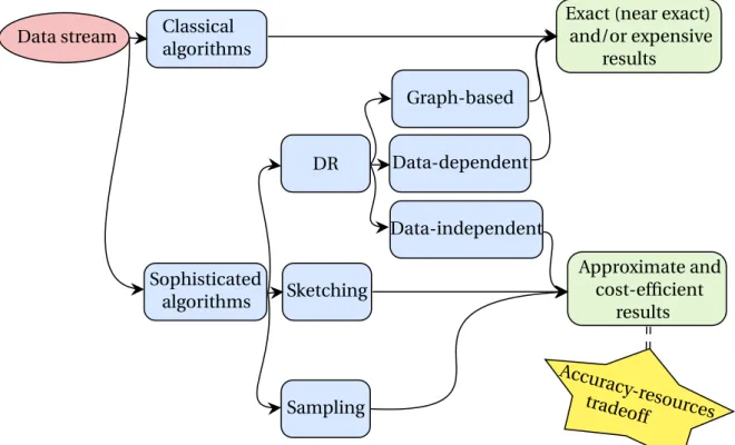
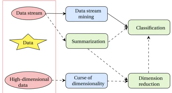
1.3 Contributions Data stream High-dimensional data Data stream mining Curse of dimensionality Summarization Classification Dimension reduction Data

Figure 1.2: The thesis context. A data stream mining task can be applied on infinite data streams, a very popular task is classification. In order to alleviate the resource cost of a given classifier, a summarization technique is sometimes used to keep synopsis information about the stream for learning. Moreover, to overcome the curse of dimensionality, a dimensionality reduction technique can be applied on high-dimensional data as an internal pre-processing technique; then, the low-dimensional representation is fed to a classification task.

Our thesis purpose is motivated by the desired criteria, described above, for IoT data stream mining. We focus mainly on the classification task and aim to develop novel stream classification approaches to improve the performance of existing algorithms using summarization techniques. Figure1.2illustrates the context of this thesis.

Dimensionality reduction, embedding, and manifold learning are names for tasks that are similar in spirit. DR is defined as the projection of high-dimensional data into a low-dimensional space by reducing the input features to the most relevant ones. Indeed, DR is crucial to avoid the curse of dimensionality – which may increase the use of computational resources and negatively affect the predictive performance of any mining algorithm. To mitigate this drawback, several reduction techniques have been proposed, and widely investigated, in the offline setting [15,16] to handle high-dimensional data. However, these techniques do not adhere to the strict computational resources requirements of the data stream learning framework [17,18]. More details are provided in the next chapter.

1.3 Contributions

The main research line of this thesis addresses the aforementioned issues about mining algorithms’ performance for IoT data streams. This thesis contributes to the stream mining field by introducing and exploring novel approaches that reduce the computational

(29)

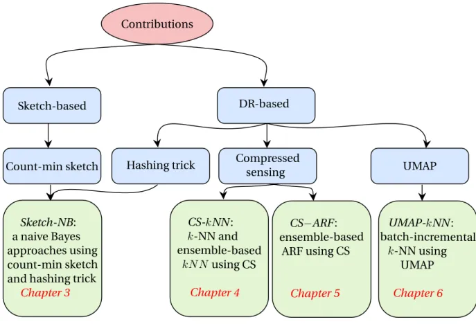
Contributions Sketch-based UMAP-kNN : batch-incremental k-NN using UMAP Chapter 6 DR-based UMAP Compressed sensing Hashing trick Count-min sketch CS−ARF : ensemble-based ARF using CS Chapter 5 CS-kNN : k-NN and ensemble-based kN Nusing CS Chapter 4 Sketch-NB: a naive Bayes approaches using count-min sketch and hashing trick

Chapter 3

Figure 1.3: Contributions of the thesis.

resources of existing algorithms while sacrificing a minimal amount of accuracy.

During this introductory, we divide the objective of the thesis in three main research questions, enumerated in the following:

• Q1: How can we improve the performance of the existing classifiers in terms of

computational resources while maintaining good accuracy?

• Q2: How can we do better by dynamically adapting to high-dimensional data streams? • Q3: How can we address concept drifts, i.e., the fact that stream distribution might

change over time?

In the following, we briefly sum up our contributions and schematize them in Figure1.3.

• In Chapter3, we aim to improve the performance of naive Bayes by developing three novel approaches to make it efficient and effective with high-dimensional data.

(30)

1.3 Contributions

– We study an efficient data structure, called Count-Min Sketch (CMS) [19], to keep synopsis (frequencies) of data in memory.

– We propose a new sketch-based naive Bayes that uses CMS to store information about the infinite amount of data streams in fixed memory size for the naive Bayes learner.

– Theoretical guarantees over the size of the CMS table are provided by extending the guarantees of the CMS technique.

– To handle high-dimensional data, we add an online pre-processing step during which data will be compressed using a rapid DR technique, such as the hashing

trick [20], before the learning tasks. This pre-processing task makes the approach faster.

– We incorporate in the learning phase an adaptive strategy using ADaptive WINdowing (ADWIN) [21], a change detector, for the entire sketch table, in order to track drifts (change in the distribution of data over time).

• In Chapter4, we focus on the k-Nearest Neighbors (kNN) algorithm [22]. We propose two approaches that aim to improve the computational costs of the kNN algorithm when dealing with high-dimensional data streams by exploring the Compressed Sensing

(CS) [23] technique to reduce the space size.

– We propose a new kNN algorithm to support evolving data stream classifica-tion, compressed-kNN. Our main focus consists of improving kNN resource performance by compressing input streams using the CS before applying the classification task. This will result in a huge reduction in the computational cost of the standard kNN.

– We provide theoretical guarantees over the neighborhood preservation before and after projection using the CS technique. We therefore ensure that the result of the classification accuracy to measure the performance of compressed-kNN is almost the same as the one that would be obtained with kNN using the high-dimensional input data.

– We also provide an ensemble technique based on Leveraging Bagging [24] where we combine several compressed-kNN results to enhance the accuracy of a single classifier.

• In Chapter5, we aim to improve the performance of the new reputed ensemble-based method, Adaptive Random Forest (ARF) [25] with high-dimensional data.

– We propose a novel ensemble approach to support high-dimensional data stream classification which aims to enhance the resource usage of the ARF ensemble method by reducing the dimensionality of the input data using the CS technique internally which are afterward fed to the ensemble members.

(31)

• In Chapter6, we explore a new DR technique that has attracted a lot of attention recently: Uniform Manifold Approximation and Projection (UMAP) [26]. We use this technique to pre-process the data, leveraging the fact that it preserves the neighborhood, to improve the results of the neighborhood-based algorithm, kNN.

– We propose an adaptation of UMAP for evolving data streams, i.e., a batch-incremental manifold learning technique. Instead of applying this batch method, UMAP, on a static dataset at once, we adapt it by using mini-batches from the stream incrementally.

– We propose a new batch-incremental kNN algorithm for stream classification using UMAP. The core idea is to apply the kNN algorithm on mini-batches of low-dimensional data obtained from the pre-processing DR step.

1.4 Publications

Some of the research findings presented in this thesis have been presented at international conferences. In the following we provide the list of currently accepted publications:

• Maroua Bahri, Silviu Maniu, Albert Bifet. “Sketch-Based Naive Bayes Algorithms for Evolving Data Streams”. In the IEEE International Conference on Big Data (Big Data), 2018, Seattle, WA, USA.

• Maroua Bahri, Albert Bifet, Silviu Maniu, Rodrigo Fernandes de Mello, Nikolaos Tziortziotis. “Compressed k-Nearest Neighbors Ensembles for Evolving Data Streams”.

In the 24th European Conference on Artificial Intelligence (ECAI), 2020, Santiago de

Compostela, Spain.

• Maroua Bahri, Bernhard Pfahringer, Albert Bifet, Silviu Maniu. “Efficient Batch-Incremental Classification for Evolving Data Streams”. In the Symposium on Intelligent

Data Analysis (IDA), 2020, Lake Constance, Germany.

• Maroua Bahri, Heitor Murilo Gomes, Albert Bifet, Silviu Maniu. “CS-ARF: Compressed Adaptive Random Forests for Evolving Data Stream Classification”. In the International

Joint Conference on Neural Networks (IJCNN), 2020, Glasgow, UK.

• Maroua Bahri, Heitor Murilo Gomes, Albert Bifet, Silviu Maniu. “Survey on Feature Transformation Techniques for Data Streams”. In the International Joint Conference on

Artificial Intelligence (IJCAI), 2020, Yokohama, Japan.

• Maroua Bahri, João Gama, Albert Bifet, Silviu Maniu, Heitor Murilo Gomes. “Data Stream Analysis: Foundations, Progress in Classification and Tools”. under review.

(32)

1.5 Outline

1.5 Outline

The thesis is structured in the following parts:

• The first part includes Chapter1– the current chapter – and Chapter2. In this chapter, we introduced the motivation of the thesis subject followed by the main goals and contributions. In Chapter2, we introduce the fundamental concepts related to the stream setting. We define data streams and cover the challenges imposed by their infinite and online nature. We present the methodologies used to process these data and survey the state-of-the-art of classification and summarization (mainly dimensionality reduction) techniques that handle evolving data streams.

• The second part covers the main body of the thesis which includes our main contributions. It is divided in four chapters. The order of the chapters does not necessarily follow the chronology of the research thesis itself. Chapter 3explores the naive Bayes algorithm, count-min sketch technique, and the hashing trick. We propose three algorithms that handle efficiently high-dimensional streams and detect drifts. In Chapter4, we focus on enhancing the computational resources of the kNN algorithm – which is very costly in practice. We present an approach that uses the compressed sensing, CS-kNN, to pre-process incrementally the stream before the classification task. We proved that the neighborhood is preserved after the projection, i.e., the accuracy is not going to be greatly impacted. We therefore used this approach as a base learner inside the Leveraging Bagging ensemble, in order to improve accuracy of the single CS-kNN. Following the same direction, Chapter5introduces a recent ensemble-based method, ARF, that induces diversity to the ensemble members (that are different from each other) by using different random projection matrices, one for each ensemble member. In Chapter6, we explore a recent dimensionality reduction technique, UMAP. Motivated by its high-quality results, we extend UMAP to the stream setting by adapting a batch-incremental strategy with the kNN algorithm to obtain the UMAP-kNN approach.

• In the third part, composed of Chapter7, we give a summary of the results achieved in this thesis, and discuss possible future developments.

• Finally, AppendixAcovers the open source frameworks that have been used to develop and test the aforementioned contributions.

(33)

(34)

2

Stream Setting: Challenges, Mining

and Summarization Techniques

Contents

2.1 Introduction . . . . 16

2.2 Preliminaries . . . . 17

2.2.1 Processing . . . 17

2.2.2 Summarization . . . 19

2.3 Stream Supervised Learning . . . . 20

2.3.1 Frequency-Based Classification . . . 22 2.3.2 Neighborhood-Based Classification . . . 22 2.3.3 Tree-Based Classification . . . 22 2.3.4 Ensembles-Based Classification . . . 23 2.4 Dimensionality Reduction . . . . 24 2.4.1 Data-Dependent Techniques . . . 26

Principal Components Analysis . . . 26

Multi-Dimensional Scaling . . . 27

Auto-Encoder . . . 27

Linear Discriminant Analysis . . . 28

Maximum Margin Criterion . . . 28

2.4.2 Data-Independent Techniques . . . 29

Random Projection . . . 29

(35)

Hashing Trick . . . 30

Locality Sensitive Hashing . . . 30

2.4.3 Graph-Based Techniques . . . 31

Isometric Mapping . . . 31

t-distributed Stochastic Neighbor Embedding . . . 32

Uniform Manifold Approximation and Projection . . . 32

2.5 Evaluation Metrics . . . . 32

2.6 Discussions . . . . 33

2.7 Conclusion . . . . 34

Parts of this chapter have been the subject of the two following survey papers in separate collaborations with Heitor Murilo Gomes1and João Gama2:

• M. Bahri, A. Bifet, J. Gama, S. Maniu, H.M. Gomes. “Data Stream Analysis: Foundations,

Progress in Classification and Tools” [27].

• M. Bahri, A. Bifet, S. Maniu, H.M. Gomes. “Survey on Feature Transformation

Tech-niques for Data Streams” [28] accepted to the International Joint Conference on Artificial Intelligence (IJCAI) 2020.

2.1 Introduction

In this chapter, we provide a general overview of the background of this thesis, the data streaming setting. The problems addressed in this thesis also belong to the supervised

learning field; in short, we are studying data stream classification. Handling the challenges of

the stream setting may require sophisticated algorithms composed of multiple components, such as a pre-processing task to reduce the dimensionality of input data, a drift detection mechanism for concept drifts.

Other than the standard constraints of data streams, the need of more computational resources to address further requirements arises when we deal with high-dimensional data. Classification algorithms must be coupled with summarization techniques to be effective.

This chapter is organized as follows: In Section2.2, we define the data stream setting and outline the main limitations and challenges in this area. Then, we spotlight some fundamental approaches used to keep the scalability of the stream methods, needed in order to handle continuous and potentially infinite streams. Section2.3is dedicated to the state-of-the-art in stream classification, by providing an overview of some well-known and new classification methods. In Section2.4, we survey the dimensionality reduction

1_{University of Waikato, Hamilton, New Zealand.} 2_{University of Porto, Porto, Portugal.}

(36)

2.2 Preliminaries

approaches designed to handle high-dimensional streaming data. We then highlight the key benefits of using these approaches for data stream classification algorithms.

2.2 Preliminaries

In the era of IoT, applications in different domains have seen an explosion of information generated from heterogeneous stream data sources every day. Hence, data stream mining has become indispensable in many real-world applications, e.g., social networks, weather forecast, network monitoring, spam emails filtering, call records, and more. As mentioned in the previous chapter, static and streaming data are different because the dynamic and changing environment of data streams makes them impossible to store or to scan multiple times due to their tremendous volume [17].

Definition 2.1 (Data streams). Stream, incremental or online, data S, are defined as an

unbounded sequence of multidimensional, sporadic, and transient observations (also called instances) made available along time. In the following, we assume that S = X1, . . . , XN, . . ., where each instance Xiis a vector that contains a attributes or features, denoted by Xi = (x1_i, . . . , xa

i)and N denotes the number of instances encountered thus far in the stream. In Section1.2, we presented the main research issues encountered in the streaming framework and in this section we present some well-known manners to deal with such constraints.

2.2.1 Processing

To cope with these requirements, we can use well-established methods such as processing in one-pass and summarization (e.g., sampling) [6,7,29]. We describe them below.

• One-pass constraint. With the increasing nature of the data, it is no longer possible to examine a stream of data efficiently by using multiple passes because of its huge size and the inability to examine it more than once during the course of computation. Considering this issue, results are obtained by scanning the data stream only once and update the classification model incrementally or with the assumption that data arrive in chunks (e.g., batch-incremental algorithms).

• Window models. Classification results can change over time with the fact that the data change accordingly. Since scanning the stream multiple times is not allowed, therefore, the so-called moving window techniques have been proposed to capture important contents of the evolving stream. There exists three kinds of windows which are the following [30]:

– Sliding window model: Whose size is fixed to keep the last incoming observa-tions, i.e., only the most recent observations from the data stream are stored

(37)

inside the window. As time changes, the sliding window moves over the stream while keeping the same size. The set of the last elements (t) is considered as the most recent one (see Figure2.1).

The length of the window

(t) (t-1) (t-2) (t) (t-1) (t-2)

The current landmark at time (t-13)

(w)

The weight

(t) Figure 2.1: Sliding window model.

– Landmark window model: In this model, the size of the window increases with time starting from a predefined instance, called landmark. When a new landmark is reached, all instance are removed and instances from the current landmark are kept (Figure2.2). One issue arises in a special case when the landmark is fixed from the beginning, so the window will contain the entire stream.

The length of the window

(t) (t-1) (t-2) (t) (t-1) (t-2)

(w)

The weight

(t) Figure 2.2: Landmark window of size 13.

– Damped window model: This model is based on a fading function that periodi-cally modifies the weights of instances. The key idea consists in assigning a weight to each instance from the stream, which is inversely proportional to its age, i.e., assign more weights to the recent arrived data. When the weight of an instance exceeds a given threshold, it will be removed from the model (see Figure2.3).

(38)

2.2 Preliminaries

Table 2.1: Window models comparison.

Window Model Definition Advantages Disadvantages

Sliding process the last received instances

suitable when the interest exists only in the recent instances

ignoring part of the stream Landmark process the entire

history of the stream

suitable for one-pass classification algorithms

all the data are equally important Damped

(Fading)

assign weights to instances

suitable when the old data may affect the results

unbounded time window The length of the window

(t) (t-1) (t-2) (t) (t-1) (t-2)

(w)

The weight

(t)

Figure 2.3: Damped window model.

Table 2.1 shows a brief description of the window models with their advantages and drawbacks. Different classification methods can be adapted to use the above models; the choice of the window model depends on the application needs [30].

The infinite nature of data streams makes them impossible to store due to resource constraints. In this context, how can we keep track of instances seen so far with minimal

information loss?

2.2.2 Summarization

Instead of – or in conjunction with – the previous mentioned techniques, another approach is to keep only a synopsis of summary of the information constructed from stream instances. This can be achieved by either keeping a small part of the incoming or by constructing other data structures storing a synopsis of the data. In what follows, we briefly present some techniques.

• Sampling. Sampling methods are the most simple ones for synopsis construction in the stream framework. Storing static datasets is simple enough. In contrast, when dealing with large data streams, this is an impossible task. In this context, it is intuitively reasonable to sample the stream in order to keep some “representative” instances and

(39)

thus decrease the stream size that will be stored in memory [31]. This method is easy conceptually and efficient to implement; however, the samples can be biased and not too representative.

• Histograms. Histograms are widely used with static datasets but their extensions to the stream framework is still a challenging task. Some techniques [32] have proposed histograms for the incremental setting to handle evolving streams. However, they do not always work because the distribution of the instances is assumed to be uniform which is not always true.

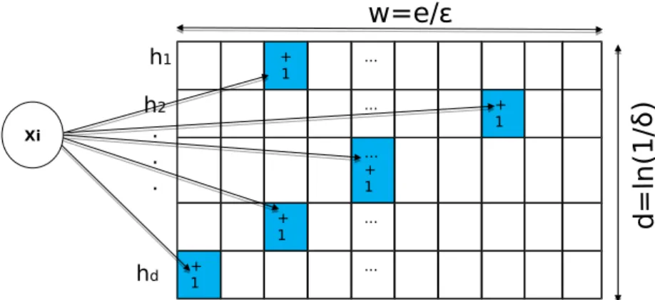
• Sketching. Sketch-based methods are well-known for keeping small, but approximate, synopses of data [33,31]. They build a summary of data stream using a small amount of memory. Among them, we cite the count-min sketch [19] which is a generalization of bloom filters [34] used for counting items of a given item, using approximate counts while keeping sound theoretical bounds on the counts.

• Dimensionality reduction. Dimensionality reduction (DR) is a very popular tool to tackle high-dimensional data, another factor that makes classification algorithms expensive. It is defined as the transformation that maps instances from a high-dimensional space onto a lower-high-dimensional one while preserving the distances between instances [16]. Thus, instead of applying the classification algorithm on the high-dimensional data, we apply it on their small representation, in the low-dimensional space.

2.3 Stream Supervised Learning

One of the most important tasks in data mining is classification [5].

Definition 2.2 (Classification problem). The problem of classification, a supervised learning task, consists in one attempts to predict a class label, (y′₎_{, of some unlabeled data instance} (X′)_{composed of a vector of attributes, by applying a generated model M (trained on labeled}

data (X, y)) [35].

y′= M(X′). (2.1)

Traditionally, data mining has been performed over static datasets in the offline setting where, for the classification task, the training process is applied on a fixed size dataset and afford to read the input data several times. However, the dynamic and open-ended nature of data streams has outpaced the capability of traditional classifiers, also called batch classifiers, to be loaded into memory due to the technical requirements of the incremental environment [36]. The difference between classifiers for statics datasets (batch classifiers) and data stream classifiers resides in the way of how the learning and prediction are performed. Unlike batch learning, online learning must deal with data incrementally and

(40)

2.3 Stream Supervised Learning

Figure 2.4: The data stream classification cycle [36].

use the one-pass processing. Moreover, and most importantly, they must use a limited amount of time to allow analysis of each instance without delay, and a limited amount of space to avoid storing huge amounts of data for the prediction task. Figure2.4illustrates the general model of the classification process within a data stream environment taking into account the requirements outlined above [35]:

1. The classifier receives the next training instance available from the stream (one-pass constraint).

2. The classifier processes the instance and updates the current model quickly using only a limited amount of memory.

3. The classifier predicts, in a first attempt, the class label of unlabeled instances and use them later to update the model.

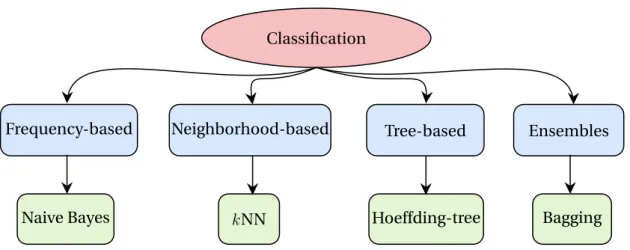
A multitude of classification algorithms for static datasets that have been widely studied in the offline processing, and proved to be of limited effectiveness when dealing with evolv-ing data streams, have been extended to work within a streamevolv-ing framework [37]. A general taxonomy divides classification algorithms into four main categories2.5: (i) frequency-based; (ii) neighborhood-frequency-based; (iii) tree-frequency-based; and (iv) ensemble-based classification algorithms.

(41)

Classification

Neighborhood-based Frequency-based

kNN Hoeffding-tree

Naive Bayes Bagging

Ensembles Tree-based

Figure 2.5: Taxonomy of classification algorithms.

2.3.1 Frequency-Based Classification

One of the most simple classifiers is Naive Bayes (NB) [38]. It uses the assumption that the attributes are all independent of each other and w.r.t. the class label, uses Bayes’s theorem to compute the posterior probability of a class given the evidence (the training data). This assumption is obviously not always true in practice, yet the NB classifier has a surprisingly strong performance in real-world scenarios. Naive Bayes is a special algorithm that needs no adaptation to the stream setting because it naturally trains data incrementally thanks to its simple and easy frequency-based strategy.

2.3.2 Neighborhood-Based Classification

k-Nearest Neighbors (kNN) is a neighborhood-based algorithm that has been adapted to the data stream setting. It does not require any work during training but it uses the entire dataset to predict the class labels for test examples. The challenge with adapting kNN to the stream setting is that it is not possible to store the entire stream for the prediction phase. An envisaged solution to solve this issue is to manage the examples that are remembered so that they fit into limited memory and to merge new examples with the closest ones already in memory. Yet, searching for the nearest neighbors still costly in terms of time and memory [39]. Another new kNN method that has been proposed recently in the stream framework is Self-Adjusting Memory kNN (samkNN) [40]. SamkNN uses a dual-memory model to capture drifts in data streams by building an ensemble with models targeting current or former concepts.

2.3.3 Tree-Based Classification

Several tree-based algorithms have been proposed to handle evolving data streams [41,

42, 43]. A well-known decision tree learner for the data streams is the Hoeffding tree algorithm [41], also known as Very Fast Decision Tree (VFDT). It is an incremental, anytime

(42)

2.3 Stream Supervised Learning

decision tree induction algorithm that uses the Hoeffding bound to select the optimal splitting attributes. However, this learner assumes that the distribution generating instances does not change over time. So, to cope with an evolving data stream, a drift detection algorithm is usually coupled with it. In [44] an adaptive algorithm was proposed, Hoeffding Adaptive Tree (HAT), extending the VFDT to deal with concept drifts. It uses the ADaptive WINdowing (ADWIN) [21], a change detector and estimator, to monitor the performance of branches on the tree and to replace them with new branches when their accuracy decreases if the new branches are more accurate. These algorithms require more memory as the tree expands and grows; they also sacrifice computational speed due to the time spent in choosing the optimal attribute to split.

2.3.4 Ensembles-Based Classification

Ensemble learning is receiving increased attention for data stream learning due to its potential to greatly improve learning performance [25,45]. Ensemble-based methods, used for classification tasks, can easily be adapted to the stream setting because of their high learning performance and their flexibility to be integrated with drift detection strategies. Unlike single classifiers, ensemble-based methods predict by combining the predictions of several classifiers. Several empirical and theoretical studies have shown the reasoning that combining multiple “weak” individual classifiers leads to better predictive performance than a single classifier [44,46,47], as illustrated in Figure2.6. Ensembles have several advantages over single classifier methods, such as: (i) robustness: they are easy to scale and parallelize; (ii) concept drift : they can adapt to change quickly by resetting or updating current under-performing model of the ensemble; and (iii) high-predictive performance: they therefore usually generate more accurate concept descriptions.

An extensive review about the related work is provided in [48], and we present briefly here the well-known and the recent ones. Online Bagging [49] is a streaming version of Bagging [46] which generates k models trained on different samples. Different from batch Bagging where samples are produced with replacement, online Bagging selects weighted samples sampled from a Poisson(1) distribution. Leveraging Bagging (LB) [24] is based on the online Bagging method. In order to increase the accuracy, LB handles drifts using ADWIN [21], where if a change is detected, the worst classifier is erased and a new one is added to the ensemble. LB also induces more diversity to the ensemble via randomization. Adaptive Random Forests (ARF) [25] is a recent extension of Random Forest method to handle evolving data streams. ARF uses Hoeffding tree as a base learner where attributes are randomly selected during training. It is coupled with a drift detection scheme using ADWIN on each ensemble member where we replace a tree, once a drift is detected, by an alternate tree trained on the new concept. Streaming Random Patches (SRP) [50] is also a novel method that combines random subspaces and bagging while using a strategy to detect drifts similar to the one introduced in [25].

(43)

Data Base classifier 1 Base classifier 2 Base classifier e ...

Decision 1 Decision 2 Decision e

Fusion

Ensemble classifier

Figure 2.6: Ensemble classifier.

One notable issue related to the ensemble-based methods with evolving data streams is the massive computational demand (in terms of memory usage and running time). Ensembles require more resources than single classifiers which become significantly worse with high-dimensional data streams.

Ensemble-based methods pose a resources-accuracy tradeoff, they produce better predictive performance than single classifiers, indeed, at the price of being more costly in terms of computational resources.

2.4 Dimensionality Reduction

Definition 2.3 (Dimensionality reduction). Given an instance Xi which is composed of a vector of a attributes Xi = x1i, . . . , xai. The DR comprises the process of finding some transformation function (or map) A : Ra _{→ R}m_{, where m ≪ a, to be applied on each} instance Xifrom the stream S as follows:

Yi = A(Xi), (2.2)

where Yi = yi1, . . . , yim.

We distinguish two main different dimensionality reduction categories: (i) feature

selection which consists in selecting a subset of the input features, i.e., the most relevant

and non-redundant features, without operating any sort of data transformation [51]; and (ii) feature transformation – also called feature extraction – which consists in constructing from a set of input features in high-dimensional space, a new set of features in a lower

(44)

2.4 Dimensionality Reduction Dimensionality reduction Data-independent Data-dependent CS HT LSH RP AE MDS

PCA LDA MMC Isomap

graph-based

tSNE UMAP

Figure 2.7: Taxonomy of dimensionality reduction techniques.

dimensional space [52].

Feature transformation and feature selection have different processing requirements. Despite the fact that both reductions are used to minimize an input feature space size, feature transformation is a DR that creates a new subset – or combinations – of features by exploiting the redundancy and noise of the input set of features, whereas feature selection is characterized by keeping the most relevant attributes from the original set of features present in the data without changing them.

Some recent surveys on streaming feature selection have been proposed [53,54,55,

56]. The major weakness of this category is that it could lead to a data loss. The latter may happen when, unintentionally, we remove features that might be useful for a later task (e.g., classification, visualization). In the following, we review the most crucial feature transformation techniques that are – or can be – used in the stream framework and discuss their similarities and differences. In what follows, we refer to feature transformation as dimensionality reduction.

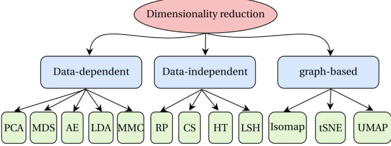
A Taxonomy of Dimensionality Reduction. In the following, we introduce DR tech-niques that have been widely used in machine learning algorithms. These techtech-niques operate by transforming and using the most relevant feature combinations, in turn reducing space and time demands; this can be crucial for applications such as classification and visualization. Traditionally, many techniques have been proposed and thoroughly used in the offline framework for static datasets, but these techniques cannot be used in the streaming framework, due to the requirements imposed by the latter (e.g., one-pass processing). Figure2.7shows a taxonomy that subdivides the DR techniques as follows,

dependent, independent, and graph-based transformation techniques. The

data-dependent techniques are derived from the whole data to achieve the transformation, whereas the data-independent techniques are based on random projections and do not

(45)

use the input data to perform the projection. Graph-based techniques are also data-dependent that build a neighborhood graph to maintain the data structure (i.e., preserves the neighborhood after projection).

2.4.1 Data-Dependent Techniques

Data-dependent techniques construct a projection function – or matrix – from the data. This requires the presence of the entirety – or at least a part of – the dataset. In the streaming context, where data are potentially infinite, the classical techniques from this category are therefore limited, since keeping the entire data stream in memory is impractical.

Principal Components Analysis

Principal Components Analysis (PCA) is the most popular and straightforward unsupervised technique that seeks to reduce the space dimension by finding a lower-dimensional basis in which the sum of squared distances between the original data and their projections is minimized, i.e. being as close as possible to zero while maximizing the variances between the first components. Mathematically, PCA aims to find a linear mapping formed by a few orthogonal linear combinations, also called eigenvectors or PCs, from the original data that maximizes a certain cost function. However, PCA computes eigenvectors and eigenvalues from a computed covariance matrix, relying on the whole dataset. This is ineffective for streaming data since a re-estimation of the covariance matrix from scratch for new observations is unavoidable.

In this context different variations of component analysis have been adapted to the stream setting. For instance, Incremental PCA (IPCA) [57] focuses on how to update the eigenvectors of images (eigenimages) based on the previous coefficients. Candid Covariance-free Incremental PCA (CCIPCA) [58] is another extension that updates the eigenvectors incrementally and does not need to compute the covariance matrix for each new incoming instance (images) which makes it very fast. The main difference among these techniques arises in how the eigenvectors are updated. On the other hand, the common limitation concerns their application domain since both techniques deal with images as high-dimensional vectors and have not been tested on different types of data [57,58]. Ross, Lim, Lin, and Yang proposed a batch-incremental PCA that deals with a set of new instances each time a batch is complete. However, this approach is not suited for instance-incremental learning (i.e., processing instances one by one incrementally). Mitliagkas, Caramanis, and Jain proposed a memory-limited streaming PCA that attempts to make vanilla PCA incremental and computation-efficient with high-dimensional data where samples are drawn from a Gaussian spiked covariance model. A more recent work [61] proposes a single-pass randomized PCA technique that iteratively update the subspace’s orthonormal basis matrix within an accuracy-performance tradeoff. Yu, Gu, Li, Liu, and Li claim that this

(46)

2.4 Dimensionality Reduction

technique works well in many applications, albeit it has been evaluated on a single image dataset.

The above PCA techniques apply to data stream mining algorithms to alleviate their computation costs. For instance, Feng, Yan, Ai-ping, and Quan-yuan proposed an efficient online classification algorithm, FIKOCFrame, that uses a PCA variant, fast iterative kernel PCA [63], to incrementally reduce the dimensionality before classification.

Cardot and Degras proposed recently a comparative review of the incremental PCA approaches where they provide guidance for selecting the appropriate approach based on their accuracy and computation resources (time and memory).

Multi-Dimensional Scaling

Multi-Dimensional Scaling (MDS) [65] is a well-known unsupervised technique used for embedding. It projects a given distance matrix into a non-linear lower-dimensional space while preserving the similarity among instances. Nevertheless, this technique is computationally expensive with large datasets and non-scalable because it requires the entire data distance matrix. To cope with this issue, some incremental versions have been proposed to alleviate the computational requirements.

Incremental MDS (iMDS) technique, proposed by Agarwal, Phillips, Daumé III, and Venkatasubramanian, keeps some distance preservation using the so-called out of sample mapping without the need of reconstructing the whole matrix. A more recent work by Zhang, Huang, Mueller, and Yoo proposed a new version of MDS for high-dimensional data, named

scMDS. It is a batch-incremental technique where authors introduced a realignment matrix

for each batch to overcome the concept drift that may occur because each batch may have a different feature bases. Nevertheless, the efficiency of this batch-incremental technique depends on the size of the batch.

Auto-Encoder

Auto-Encoders (AEs) [68] are a family of Neural Networks (NNs) which are designed for unsupervised learning, for learning a low-dimensional representation of a high-dimensional dataset, where the input is the same as the output. An AE has two main components, (i) the encoder step, during which the input data are compressed into a latent space representation; and (ii) the decoder step where the input data are reproduced from this new representation. Vincent, Larochelle, Bengio, and Manzagol introduced the denoising AE (DAE), a variant of AE, that extracts features by adding perturbations to the input data and then attempts to reconstruct the original data. Zhou, Sohn, and Lee proposed an online DAE that adaptively uses incremental feature augmentation, depending on the already existing features, to track drifts. However, this work does not address the convergence properties of the training task (the hyperparameters configuration used to construct the network, e.g., the number of epochs) that are crucial in the stream setting.

(47)

Unlike other algorithms, NNs naturally handle incremental learning tasks [71]. While dealing with data streams, NNs learn by passing the data in smaller chunks (Mini-Batch Gradient Descent) or an instance at a time (Stochastic Gradient Descent). Using this way, each instance is going to be processed only once without being stored. The advantage of using this kind of technique is that it is not limited to linear transformations. Non-linearities are introduced using non-linear activation functions, NNs are therefore more flexible. Nevertheless, this high-quality results that this family of learners offers come at the price of slow learning speed due to the infinite nature of data and the large parameter space needed.

Linear Discriminant Analysis

Linear Discriminant Analysis (LDA) [72], also known as Fisher Discriminant Analysis (FDA), is a linear transformation technique. Contrary to the techniques mentioned earlier, LDA performs a supervised reduction that takes into account the class labels of instances by looking for efficient discrimination of data in a way to maximize the separation of the existing categories (class labels), while other techniques, e.g. PCA, aim at an efficient representation. However, when dealing with evolving data streams, the set of labels of instances may be unknown at each learning stage because new classes may appear (concept evolution) [73]. One way to cope with this issue is to update the discriminant eigenspace when a new class arrives, as introduced in the Incremental LDA (ILDA) approach [74]. Another streaming extension of LDA has been proposed, called IDR/QR [75]. It applies a singular value decomposition suitable for large datasets that uses less computational cost than ILDA. Kim, Stenger, Kittler, and Cipolla proposed an ILDA that incrementally updates the discriminant components using a different criterion. They claim to be more efficient in terms of time and memory than the previous approaches.

Maximum Margin Criterion

Maximum Margin Criterion (MMC) [77] is a supervised feature extractor technique based on the same representation of LDA while maximizing a different objective function. To overcome the limitations of MMC with streaming data, Yan, Zhang, Yan, Yang, Li, Chen, Xi, Fan, Ma, and Cheng proposed an Incremental MMC (IMMC) approach, which infers an online adaptive supervised subspace from data streams by optimizing the MMC and updating the eigenvectors of the criterion matrix incrementally. Hence, the computation of IMMC is very fast since it does not need to reconstruct the criterion matrix when new instances arrive.

The incremental formulation of the proposed algorithm is mentioned in [78] with the proof. A major drawback of this approach is its sensitivity to parameter setting.

(48)

2.4 Dimensionality Reduction

2.4.2 Data-Independent Techniques

Data-independent techniques are mainly based on the principle of random projections. These techniques are therefore appropriate for evolving streams because they generate the projection matrices (or functions), and transform data into a low-dimensional space, independently from the input data.

Random Projection

Random projection is a powerful technique for dimensionality reduction that has been widely applied with several mining algorithms for solving numerous problems [79]. RP is based on the Johnson-Lindenstrauss (JL) Lemma2.4.2[80] which asserts that N instances from a Euclidean space can be projected into a lower-dimensional space of O(log(N/ϵ2₎₎ dimensions under which pairwise distances are preserved within a multiplicative factor of 1 ± ϵ[81].

Let ϵ ∈ [0, 1], S = {X1, ..., XN} ∈ Ra. Given a number m ≥ log(N/ϵ2), ∀Xi, Xj ∈ S there is a linear map A : Ra→ Rm_{such that:}

(1 − ϵ)∥Xi− Xj∥22 ≤ ∥AXi− AXj∥22≤ (1 + ϵ)∥Xi− Xj∥22, (2.3)

where A is a random matrix that can be generated using, e.g., a Gaussian distribution. Hence, RP offers a computationally-efficient and straightforward way to compress the dimensionality of input data rapidly while approximately preserving the pairwise distances between any two instances.

Compressed Sensing

Compressed Sensing (CS), also called compressed sampling, technique based on the principle that a data compression method has to deal with redundancy while transforming and reconstructing data [23]. Given a sparse/high-dimensional vector X ∈ Ra_{, the goal of} CS is to measure Y ∈ Rm_{and then reconstruct X, for m ≪ a, as follows:}

Y = AX, (2.4)

where A ∈ Rp×d_{is called a measurement, (sampling, or sensing ) matrix.}

The technique has been widely studied and used throughout different domains in the offline framework, such as image processing [82], face recognition [83], and vehicle classification [84]. The basic idea is to use orthogonal features to provably and properly represent sparse and high-dimensional vectors X ∈ Ra_{as well as reconstruct them from a} small number of feature vectors Y ∈ Rm_{, where m ≪ a. Two main concepts are crucial the} stream recovery with high probability [23]:

(49)

Sparsity: CS exploits the fact that data may be sparse and hence compressible in a

concise representation. For an instance X with support supp(X) = {l : xl _{̸= 0}, we define} the ℓ0-norm ∥X∥0 = |supp(X)|, so X is s-sparse if ∥X∥0 ≤ s. The implication of sparsity is important to remove irrelevant data without much loss.

Restricted Isometry Property (RIP): A is said to respect the RIP for all s-sparse data if

there exists ϵ ∈ [0, 1] such that:

(1 − ϵ)∥X∥2₂≤ ∥AX∥2

2 ≤ (1 + ϵ)∥X∥22, (2.5)

where X ∈ S. This property holds for all s-sparse data X ∈ Ra_.

RP and CS are closely related. Random matrices (e.g., Bernoulli, Binomial, Gaussian) are also known to satisfy the RIP with high probability if m = O(s log(a)) [85], which is essentially a JL type condition on projections using the sensing matrix A. The difference is mainly in terms of how big the matrix A has to be.

Hashing Trick

Hashing trick (HT) [20], also known as feature hashing, is a fact and space-efficient technique that projects sparse instances or vectors into a lower feature space using a hash function. Given a list of keys that represents a set of features from the input instances, it computes then the hash function for each key, which will ensure its mapping to a specific cell of a fixed size vector that constitutes the new compressed instance.

An important point to make is that, generally, the quality of models changes when the size of the hash table increases. Usually, the larger the hash table size is, the better is the model. However, an optimal point can be picked which guarantees almost perfect model, while the output dimension size is not to be very large. The HT technique has the appealing properties of being very fast, simple, and sparsity preserving. A significant advantage to point out is that this technique is very memory-efficient because the output feature vector size is limited, making it a clear candidate for using, especially for online learning on streams.

Locality Sensitive Hashing

The basic idea behind the Locality Sensitive Hashing (LSH) [86] is the application of hashing functions which map, with high probability, similar instances (in the high-dimensional

d-space) that have the same hash code to the same bucket. I.e., if instances are phrases that are very similar to each other, they might be different by only one or a couple of words or even one character; hence, LSH will generate very similar, ideally, identical hash codes to increase the probability of collision for those instances. LSH operates by partitioning the space with hyperplanes into disjoint regions, which are spatially proximate. A particular hyperplane is going to cut the space into two half-spaces, and arbitrarily one side is called positive “1” and the other side negative “0”; this will help in classifying the instances for that

Improving IoT data stream analytics using summarization techniques

HAL Id: tel-02865982

https://tel.archives-ouvertes.fr/tel-02865982

summarization techniques

Maroua Bahri

To cite this version:

NNT

:2020IPP

A

T017

Improving IoT Data Stream Analytics

Using Summarization Techniques

M

B

Using Summarization Techniques

Maroua Bahri

A thesis submitted in fulfillment of the requirements for the degree of

Doctor of Philosophy

Télécom Paris

Institut Polytechnique de Paris

Supervisors:

Albert Bifet

Silviu Maniu

Examiners:

João Gama

Cédric Gouy-Pailler

Ons Jelassi

Moamar Sayed-Mouchaweh

Mauro Sozio

Maguelonne Teisseire

Paris, 2020

Abstract

I dedicate to my sweet loving

Father, Mother & Siblings

whose unconditional love, encouragement, affection, and

prays of day and night make me able to get such success

and honor. Without them, I would never get through this.

Table of Contents

List of Figures

List of Tables

List of Abbreviations

List of Symbols

Part I

1

Introduction

1.1

Context and Motivation

1.2

Challenges

1.3

Contributions

1.4

Publications

1.5

Outline

2

Stream Setting: Challenges, Mining

and Summarization Techniques

2.1

Introduction

2.2

Preliminaries

2.3

Stream Supervised Learning

2.4

Dimensionality Reduction