HAL Id: inserm-02196731
https://www.hal.inserm.fr/inserm-02196731
Submitted on 29 Jul 2019
HAL is a multi-disciplinary open access archive for the deposit and dissemination of sci-entific research documents, whether they are pub-lished or not. The documents may come from teaching and research institutions in France or abroad, or from public or private research centers.
L’archive ouverte pluridisciplinaire HAL, est destinée au dépôt et à la diffusion de documents scientifiques de niveau recherche, publiés ou non, émanant des établissements d’enseignement et de recherche français ou étrangers, des laboratoires publics ou privés.
for the upper part of glycolysis
Anamya Nagaraja, Nicolas Fontaine, Mathieu Delsaut, Philippe Charton,
Cedric Damour, Bernard Offmann, Brigitte Grondin-Perez, Frédéric Cadet
To cite this version:
Anamya Nagaraja, Nicolas Fontaine, Mathieu Delsaut, Philippe Charton, Cedric Damour, et al.. Flux prediction using artificial neural network (ANN) for the upper part of glycolysis. PLoS ONE, Public Library of Science, 2019, 14 (5), pp.e0216178. �10.1371/journal.pone.0216178�. �inserm-02196731�
Flux prediction using artificial neural network
(ANN) for the upper part of glycolysis
Anamya Ajjolli Nagaraja1, Nicolas Fontaine2, Mathieu Delsaut1, Philippe Charton
ID3,
Cedric Damour1, Bernard Offmann4, Brigitte Grondin-Perez1, Frederic CadetID3*
1 LE2P, Laboratory of Energy, Electronics and Processes EA 4079, Faculty of Sciences and Technology,
University of La Reunion, France, 2 PEACCEL, n˚6 Square Albin Cachot, Paris, France, 3 DSIMB, INSERM, UMR S-1134, Laboratory of ExcellenceLABEX GR, Faculty of Sciences and Technology, University of La Reunion & University Paris Diderot, Paris, France, 4 Universite´ de Nantes, Unite´ Fonctionnalite´ et Inge´nierie des Prote´ines (UFIP), UMR 6286 CNRS, UFR Sciences et Techniques, chemin de la Houssinière, France
Abstract
The selection of optimal enzyme concentration in multienzyme cascade reactions for the highest product yield in practice is very expensive and time-consuming process. The model-ling of biological pathways is a difficult process because of the complexity of the system. The mathematical modelling of the system using an analytical approach depends on the many parameters of enzymes which rely on tedious and expensive experiments. The artifi-cial neural network (ANN) method has been successively applied in different fields of sci-ence to perform complex functions. In this study, ANN models were trained to predict the flux for the upper part of glycolysis as inferred by NADH consumption, using four enzyme concentrations i.e., phosphoglucoisomerase, phosphofructokinase, fructose-bisphosphate-aldolase, triose-phosphate-isomerase. Out of three ANN algorithms, the neuralnet package with two activation functions, “logistic” and “tanh” were implemented. The prediction of the flux was very efficient: RMSE and R2were 0.847, 0.93 and 0.804, 0.94 respectively for logis-tic and tanh functions using a cross validation procedure. This study showed that a systemic approach such as ANN could be used for accurate prediction of the flux through the meta-bolic pathway. This could help to save a lot of time and costs, particularly from an industrial perspective. The R-code is available at: https://github.com/DSIMB/ANN-Glycolysis-Flux-Prediction.
Introduction
The emergence of genomics, transcriptomics and proteomics, along with improvements in information technology, helped us to integrate the information, build the mathematicalin sil-ico model of a biological system and observe its behaviour [1–5]. The integration of different “-omics” data helped us to understand the genetic difference between the phenotypes, to iden-tify the molecular signature [6,7] and use metabolic engineering [8,9] etc. There have been many attempts to model biological systems, likeSaccharomyces cerevisiae [4,10–12], Escheri-chia coli [13–15], other organisms [3] and many plant metabolic networks for observing and predicting the behaviour of a system using different methods [2,16].
a1111111111 a1111111111 a1111111111 a1111111111 a1111111111 OPEN ACCESS
Citation: Ajjolli Nagaraja A, Fontaine N, Delsaut M,
Charton P, Damour C, Offmann B, et al. (2019) Flux prediction using artificial neural network (ANN) for the upper part of glycolysis. PLoS ONE 14(5): e0216178.https://doi.org/10.1371/journal. pone.0216178
Editor: Marie-Joelle Virolle, Universite Paris-Sud,
FRANCE
Received: January 28, 2019 Accepted: April 15, 2019 Published: May 8, 2019
Copyright:© 2019 Ajjolli Nagaraja et al. This is an open access article distributed under the terms of theCreative Commons Attribution License, which permits unrestricted use, distribution, and reproduction in any medium, provided the original author and source are credited.
Data Availability Statement: All relevant data are
within the manuscript and its Supporting Information files.
Funding: AAN is supported by a PhD grant from
Region Reunion and European Union (FEDER) under European operational program INTERRG V-2014-2020 file number 20161449, tiers 234273.
Competing interests: The authors have declared
Many different kinds of mathematical models exist to study biological systems [17,18]. Sev-eral approaches have been developed to determine or estimate the flux through the metabolic pathway [19–21]. Based on the data and constraints used, the mathematical modelling can be classified into two broad categories [2,16] i.e., kinetic modelling or mechanistic modelling [22–24], and constraint-based or stoichiometric modelling [12,25,26]. The kinetic model defines the reaction mechanism in the system using kinetic parameters to evaluate rate laws. These rate laws are defined from the experiment, assuming that the experimental conditions are similar toin-vivo conditions [27]. To build a kinetic model, the system has been made as simple as possible, while retaining system behaviour. The modelling of enzymes like phospho-fructokinase could be problematic and might need more parameters than other enzymes [28]. Determining the kinetic parameter is expensive and time consuming; some parameters could be more difficult to measure. Although many enzymatic assays are described in the literature, sometimes it is necessary to modify the assay for new enzymes or to find a new one. In some cases, for example, following enzyme reaction through spectrophotometers or spectrofluorim-eters, this is difficult due to no absorption or emission signals [29] linked to the reactants. Most of the available kinetic data are obtained fromin-vitro studies using purified enzymes
which might not represent the exact properties ofin-vivo enzymes [23]. For example: The Vmaxvalue measuredin vitro may not represent the value of an in vivo system because of the
destruction of enzyme complexes, cellular organisation and the absence of an unknown inhibi-tor or activainhibi-tor [30,31]. A constraint-based model uses physiochemical constraints like mass balance, thermodynamic constraints, etc., in the modelling, to observe and study the behaviour of the system [25]. There are different methods, like flux balance analysis [32] and metabolic flux analysis [33]. Flux balance analysis is an approach to studying biochemical networks on a genomic scale, which includes all the known metabolite reactions, and the genes that encode for a particular enzyme. The data from genome annotation or existing knowledge is used to construct the network [5,34] and the physicochemical constraints are used to predict the flux distribution, considering that the total product formed must be equal to the total substrate consumed in steady state conditions [32]. This method is used to predict the growth rate [5,32,34,35] or the production of a particular metabolite [36]. Metabolic flux analysis, an experimental based method, allows the quantification of metabolite in the central metabolism using the Carbon-labelled substrate [33,37,38]. The labelled substrate is allowed to distribute over the metabolic network and is measured using NMR [39] or mass spectrometry [32].
Many of the biomolecules like organic acids [40,41], antibiotics [42–44], bioethanol etc. [45,46] have been used in the pharmaceutical and food industries and as energy sources. Bio-molecule production is attracting the attention of biologists and industries due to the decrease in non-renewable resources and global warming [47,48]. Synthetic biology and systems biol-ogy help to obtain the highest yield of biomolecules from the source [49–51].
Glycolysis is the centre of the metabolic system in all living organisms. It is an anaerobic pathway present in almost all living cells and helps in ATP generation. Glycolysis has been established as the central core for the fermentation. It contributes to the production of differ-ent metabolites, like citric acid, succinic acid, amino acids, etc., through pyruvate, the end product of glycolysis [52].
The neural network is an architecture, modelled on the brain, that is organized with neu-rons and synapses present in a structure of nodes (formal neuron) connected together [53,54]. Each numerical input corresponds to the input layer, and the value to predict (variable to explain) corresponds to the last level, the output layer. Between those two layers, intermediary nodes are present, built specifically and in sufficient number to model the problem; they form the hidden layer. The neural network has been successfully applied in different fields of science such as physics [55,56], environmental science [57–59] and data mining [60,61] for the
Abbreviations: ANN, artificial neural network; PGI,
phosphoglucoisomerase; PFK,
6-phosphofructokinase; FBA, fructose bisphosphate aldolase; TPI, triose phosphate isomerase; RMSE, root mean square error.
prediction of different features in the system. The ANN is also core for deep learning [62]. The artificial neural network could be used to predict the product outcome (i.e. flux through the pathway) when combined with Flux balance analysis or other modelling approaches.
The ANN has been used earlier in predicting the fluxes from13C labelling of metabolites in mammalian gluconeogenesis by M.R. Antoniewicz et al. [21]. Three linear regression model-ling methods, multiple linear regression (MLR), principal component regression (PCR) and partial least square regression (PLS) were run on simulated data and compared to the ANN. The study showed that ANN, that requires the larger sample (>200) performed better than the other methods for flux prediction using new mass isotopomer data [21].
Due to the challenges in estimating the flux using different methods like constraint-based and kinetic-based modelling approaches [63–66], we developed a simple method using artifi-cial neural networks. This method is based purely on the existing experimental data and hence does not require kinetic parameters as in kinetic modelling and no prior information is required regarding the stoichiometry of the metabolic pathway. In this study, an artificial neu-ral network was built to estimate the flux using enzyme concentrations for the upper part of glycolysis as input. Finding the optimum enzyme concentration—which gives the highest product—through experiments is very tedious and expensive. The neural network approach could be helpful for choosing the optimum enzyme concentrations which enhance the final product concentration without experimental setup, within a short period of time. Experiments were carried out in order to:i) assess the structure of the ANN using three different
approaches,ii) evaluate different activation functions and iii) compare the prediction of flux of
NAD+to the fluxes predicted by Fievet & al. (2006).
Materials and methods
Principle of artificial neural networks
The base element of ANN is the perceptron, defined in 1958 by Rosenblatt [67]. A combina-tion funccombina-tion computes a value based on the input layer and some weights. This is a weighted sum∑nipi(observed node) of the nivalues in the input layer. To define the output value, a
function called activation function is applied to this value. We note nifor the node i, the weight
picorresponds to the connection between node i, the observed node and the activation
func-tion f, associated with the observed node (Fig 1).
The structure of an ANN is defined by the number of layers and nodes, by the way they are linked (activation function) and the method to estimate the weights.
Input for building the ANN model
The flux measurement data fromin-vitro reconstructed upper part of glycolysis [20] was used to build the artificial neural network (Fig 2). The input for the ANN model consists of concen-trations of enzymes phosphoglucoisomerase (PGI), phosphofructokinase (PFK), fructose
Fig 1. Architecture of artificial neural network. https://doi.org/10.1371/journal.pone.0216178.g001
bisphosphate aldolase (FBA) and triose phosphate isomerase (TPI) in mg/L, and the output is flux J (μM/s) measured as the NADH consumption by glycerol-3-phosphate dehydrogenase (G3PDH). The flux measured through the upper part of glycolysis is indirect and we assume that most of the NADH in the system is consumed during the measurement. The data has been normalised using min-max method before building the neural network.
Experimental details
The upper part of glycolysis was reconstructedin vitro (Fig 2), with constant concentration of hexokinase andglycerol-3-phosphate dehydrogenase, while the other four enzymes (PGI, PFK, FBA and TPI) concentrations varied. The total enzyme concentration of the four enzymes (PGI, PFK, FBA and TPI) was constant at 101.9 mg/L. The NADH consumption using the glycerol-3-phosphate dehydrogenase is monitored every 2s with Uvikon 850 spectrometer at 390 nm from 60 to 120s. The linear slope of NADH was calculated as the flux through the path-way. The assays were performed in triplicate by Fie´vet et al., 2006, at 25˚C, by adding 1mM ATP at pH 7.5. Data is given in supplementary information (Table A inS1 File).
Structure of ANN
The artificial neural network built with a single layer of hidden units [68] using statistical tool R (version 3.4.3) (R Core Team (2013). R: A language and environment for statistical comput-ing. R Foundation for Statistical Computing, Vienna, Austria.http://www.R-project.org/) using three different packages: nnet (version 7.3–12) [69], neuralnet (version 1.33) [70] and RSNNS (version 0.4–10) [71].
The network consists of three layers: a) Input (I), b) Hidden layer (H) and c) Output. These layers are connected by edges or neurons. The weighted sum of neuron inputs is submitted to a function which conditions neuron activation. There is no rule for deciding the number of neuron units in a single hidden layer; to choose the best algorithm out of three (i.e. nnet, neur-alnet and RSNNS), we first chose the number of hidden units according to Equation 1 and compared the RMSE (Equation 2) and coefficient of determination (R2) (Equation 3) values between the three methods. The algorithm with the lowest RMSE value and highest R2value during the leave-one-out cross validation was chosen as an algorithm of interest and the effect of the number of hidden units on RMSE and R2was analysed between 1 to 25 hidden units.
Fig 2. The upper part of glycolysis reconstructed in vitro. HK-hexokinase; PGI-phopshoglucoisomerase;
PFK-phosphofructokinase; FBA-fructose bisphosphate aldolase; TPI- triose phosphate isomerase; G3PDH- glycerol-3-phosphate dehydrogenase, CK- Creatine kinase.
Equation 1: Where Nh is number of hidden units; Ns: number of sampling in training data; Ni: number of input neurons; No: number of output neurons;α: arbitrary scaling factor 2–10.
Nh ¼ Ns a ðNi þ NoÞ
Equation 2: Where RMSE is root mean square error, Yi is ANN predicted values; yi is experimental values; n is number of predictions.
RMSE ¼ ffiffiffiffiffiffiffiffiffiffiffiffiffiffiffiffiffiffiffiffiffiffiffiffiffi P ðYi yiÞ 2 n i¼1 n v u u u t
Equation 3: Where R2 is coefficient of determination; Yi ANN is predicted values; yi is experimental values; n is number of predictions, Y is average of experimental values.
R2 ¼ 1 P iðyi YiÞ 2 P iðyi �yÞ 2 where; �y ¼ Pn i¼1yi n
Results and discussion
The three-neural network algorithms: nnet [69], neuralnet [70] and RSNNS [71] are built with a hidden number of units ranging from 9 to12, as shown in Equation 1. The RMSE and coeffi-cient of determination were compared between algorithms during leave-one-out cross valida-tion. Out of three algorithms, the neuralnet performed better than the other two (Table B inS1 File), allowing the option of choosing two different activation functionsi.e., logistic
(sigmoi-dal) and tanh (Equation 4 and Equation 5 respectively). Equation 4: logistic activation function.
Logistic xð Þ ¼ 1 1 þe x
Equation 5: tanh activation function.
tanh xð Þ ¼ 2 1 þe 2x 1
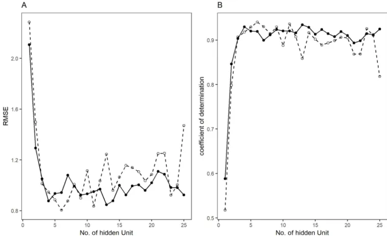
Using the neuralnet model, with “logistic” and “tanh” activation functions, the effect of the number of hidden units on RMSE and R2was studied (Fig 3) with a leave-one-out-cross-vali-dation procedure (Table C inS1 File). The logistic function with 13 hidden units gives a RMSE of 0.847, R2of 0.93 and tanh function RMSE of 0.804, and R2of 0.94 with 6 hidden units. The R-script to build the ANN with leave-one-out cross validation is given in R-Scripts A inS1 File.
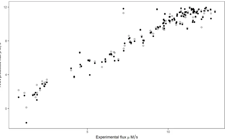
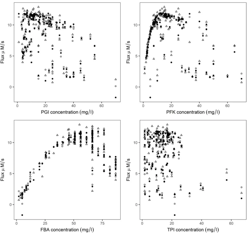
Experimental flux was compared with the ANN predicted flux by leave-one-outcross-vali-dation procedure, using chosen hidden units with logistic and tanh function (Fig 4). The effects of enzyme concentrations on the predicted flux and experimental flux were compared, and found to follow a similar trend (Fig 5).
During the cross validation of the neural network model, a negative flux value was pre-dicted for one combination of enzymes (Table 1: Index-3). This is because, during a leave-one-out procedure (LOOcv), one combination of the four enzymes is not included in the model training and has to be predicted. The negative value shows the poor ability of the ANN model to predict the outliers, i.e. a combination that is not close (in terms of PGI, PFK, FBA and TPI concentrations) to those included in the training data set.
The original study by J. B. Fievet et al. developed a model to predict flux. As the authors mentioned in their article, their flux predictor overestimates the observed flux by a constant factor. The predicted flux in their method, has an R2value of 0.86, whereas an ANN approach with logistic function showed an R2value to be 0.93 and in case of tanh activation function, an R2of 0.94, obtained with leave-one-out cross validation, which implies that the ANN approach is more efficient in predicting the flux than the method developed in the Fievet study. The effect of enzyme concentrations on the predicted flux by both methods follows a similar trend.
The difference between actual flux and ANN predicted flux was an average of 0.57μM/s for logistic and for tanh, with a standard deviation of 0.63 and 0.57 respectively (Table 1), whereas the Fievet & al. study (2006) showed an average of 3.3 and a standard deviation of 2.2 with actual predicted values. Fievet et al. stated that their method overestimates the flux values by a constant factor of 1.38. Hence by dividing the predicted flux values by 1.38, corrected values were obtained. The new average corrected value is 1.04 and standard deviation is 0.78 with the experimental values. This indicates that the ANN method performs better than the method described in the original study. This ANN-based method provides additional degrees of dom over the method proposed in Fievet & al. (2006). Indeed, the number of degrees of free-dom increases with the number of hidden units. This makes it possible to obtain an important advantage regarding the error inherent to the learning phase.
Fig 3. Effect of the number of hidden units on RMSE (A) and coefficient of determination (B) in activation function logistic (filled circle, solid line) and tanh
(open circle and dotted lines).
Conclusion
Kinetic modelling of metabolic pathways is challenging because of the difficulties in estimating the kinetic parameters [29,65], and is sometimes expensive because of the high-cost substrates and technologies involved [72,73], whereas the constraint-based model does not use any kinetic parameters but is efficient enough to predict the flux of metabolites. Choosing the opti-mum enzyme concentrations for the highest flux could be a challenge when conducting exper-iments. Using artificial intelligence with available experimental data can help us find a quicker and more cost-effective solution for biological problems.
In this study, a neural network model was built successfully with two different activation functions: i.e., logistic (sigmoidal) and tanh, with RMSE and R2values of 0.847, 0.93 and 0.804, 0.94 respectively. The difference between actual flux and ANN predicted flux was an average of 0.57 for both activation functions. The J. B. Fievet et al. method after the correction has a RMSE of 1.30, with a 1.05 difference between predicted and observed flux, which clearly indi-cates that the ANN method works better than the other method.
It has not escaped our attention that the artificial neural network model depends on the diversity of the training data, and hence training the model with a maximum of variability in the concentration of enzymes plays a crucial role. The model built in this study might not be enough to extrapolate a model for all other enzyme concentrations. In future, the study will be
Fig 4. Relationship between flux predicted by leave-one-outcross-validation and experimental flux. Filled and open circles represent logistic and tanh activation
functions respectively.
extended to predict the wide range of flux and the enzyme concentration for a particular flux. Experiments in a wet laboratory will be carried out for an upcoming application paper. Even though further work has to be performed, the artificial neural network approach is a promising method in metabolic pathway modelling and could find its place in metabolic engineering and industrial scale biomolecule synthesis.
Fig 5. Relationship between the individual enzyme concentration with experimental and ANN predicted flux. Filled circle and open circle are enzyme
concentration vs predicted flux with logistic and tanh activation functions respectively, open triangles represent the experiment.
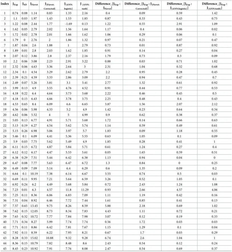
Table 1. Comparison of flux values (inμM/S) between observed flux (JExp), J.B Fievet (JFievet)and ANN predicted flux with activation functions logistic (J{ANN: logis-tic}) and tanh (J{ANN: tanh})and the standard deviation of observed flux (JSD).
Index JExp JSD JFievet J{Fievet: Corrected} J{ANN: logistic} J{ANN: tanh} Difference_[JExp: JFievet]
Difference_[JExp: J{Fievet: Corrected}] Difference_[JExp: J{ANN:logistic}] Difference_[JExp: J{ANN:tanh}] 1 0.74 0.08 1.14 0.83 1.33 2.16 0.4 0.09 0.59 1.42 2 1.1 0.03 1.97 1.43 1.53 1.85 0.87 0.33 0.43 0.75 3 1.22 0.08 2.44 1.77 -1.69 0.13 1.22 0.55 2.91 1.09 4 1.62 0.05 2.79 2.02 1.56 1.64 1.17 0.4 0.06 0.02 5 1.72 0.02 2.78 2.01 1.66 1.62 1.06 0.29 0.06 0.1 6 1.79 0 2.76 2 1.86 1.32 0.97 0.21 0.07 0.47 7 1.87 0.04 2.6 1.88 1 2.79 0.73 0.01 0.87 0.92 8 1.89 0.01 2.8 2.03 1.62 1.85 0.91 0.14 0.27 0.04 9 2.07 0.12 3.86 2.8 2.37 2.16 1.79 0.73 0.3 0.09 10 2.2 0.06 3.08 2.23 2.91 3.22 0.88 0.03 0.71 1.02 11 2.32 0.06 4.63 3.36 2.64 3 2.31 1.04 0.32 0.68 12 2.34 0.1 4.54 3.29 2.62 2.79 2.2 0.95 0.28 0.45 13 2.39 0.21 4.59 3.33 2.86 3.09 2.2 0.94 0.47 0.7 14 2.49 0.07 5.26 3.81 3.1 3.41 2.77 1.32 0.61 0.92 15 3.99 0.13 4.9 3.55 4.76 4.52 0.91 0.44 0.77 0.53 16 4.18 0.22 6.4 4.64 3.73 3.68 2.22 0.46 0.45 0.5 17 4.18 0.15 6.43 4.66 3.78 3.75 2.25 0.48 0.4 0.43 18 4.53 0.65 8.4 6.09 6.6 6.65 3.87 1.56 2.07 2.12 19 4.56 0.06 5.98 4.33 5.2 4.9 1.42 0.23 0.64 0.34 20 4.62 0.06 5.52 4 5 4.99 0.9 0.62 0.38 0.37 21 5.05 0.13 6.77 4.91 5.71 5.68 1.72 0.14 0.66 0.63 22 5.13 0.19 6.27 4.54 5.62 5.74 1.14 0.59 0.49 0.61 23 5.15 0.26 6.98 5.06 3.97 5.7 1.83 0.09 1.18 0.55 24 5.46 0.1 6.09 4.41 5.36 5.55 0.63 1.05 0.1 0.09 25 5.9 0.03 7.75 5.62 5.49 4.9 1.85 0.28 0.41 1 26 6.11 0.15 6.72 4.87 5.84 5.71 0.61 1.24 0.27 0.4 27 6.12 0.12 6.17 4.47 5.53 5.61 0.05 1.65 0.59 0.51 28 6.38 0.29 7.51 5.44 6.42 6.38 1.13 0.94 0.04 0 29 6.47 0.08 7.77 5.63 6.47 6.72 1.3 0.84 0 0.25 30 6.49 0.09 7.09 5.14 6.4 6.29 0.6 1.35 0.09 0.2 31 6.64 0.1 10.19 7.38 6.14 6.67 3.55 0.74 0.5 0.03 32 6.69 0.11 9.95 7.21 5.64 6.59 3.26 0.52 1.05 0.1 33 6.92 0.24 6.2 4.49 5.68 5.84 0.72 2.43 1.24 1.08 34 7.23 0.01 6.3 4.57 11.8 11.29 0.93 2.66 4.57 4.06 35 7.25 0.11 8.36 6.06 6.83 7.09 1.11 1.19 0.42 0.16 36 7.31 0.04 8.92 6.46 7.72 7.44 1.61 0.85 0.41 0.13 37 7.57 0.65 13.45 9.75 8.26 8.59 5.88 2.18 0.69 1.02 38 7.62 0.15 12.05 8.73 8.34 7.83 4.43 1.11 0.72 0.21 39 7.65 0.32 10.72 7.77 7.84 7.98 3.07 0.12 0.19 0.33 40 7.71 0.34 8.27 5.99 7.74 7.74 0.56 1.72 0.03 0.03 41 7.71 0.11 8.86 6.42 7.81 7.67 1.15 1.29 0.1 0.04 42 7.92 0.11 8.59 6.22 7.95 8.21 0.67 1.7 0.03 0.29 43 8.28 0.33 15.02 10.88 9.32 9.28 6.74 2.6 1.04 1 44 8.36 0.15 10.79 7.82 8.48 8.6 2.43 0.54 0.12 0.24 45 8.45 0.23 10.92 7.91 7.76 8.08 2.47 0.54 0.69 0.37 (Continued )
Table 1. (Continued)
Index JExp JSD JFievet J{Fievet: Corrected} J{ANN: logistic} J{ANN: tanh} Difference_[JExp: JFievet]
Difference_[JExp: J{Fievet: Corrected}] Difference_[JExp: J{ANN:logistic}] Difference_[JExp: J{ANN:tanh}] 46 8.46 0.11 10.49 7.6 8.03 7.43 2.03 0.86 0.43 1.03 47 8.5 0.09 8.97 6.5 8.05 8 0.47 2 0.45 0.5 48 8.9 0.06 10.03 7.27 8.94 9.2 1.13 1.63 0.04 0.3 49 8.96 0.08 10.55 7.64 9.03 8.91 1.59 1.32 0.07 0.05 50 9.08 0.35 10.97 7.95 8.56 8.85 1.89 1.13 0.52 0.23 51 9.24 0.04 8.74 6.33 9.4 9.55 0.5 2.91 0.16 0.31 52 9.31 0.1 15.81 11.46 11.75 11.71 6.5 2.15 2.44 2.4 53 9.35 0.46 12.43 9.01 9.64 9.39 3.08 0.34 0.29 0.04 54 9.39 0.22 12.52 9.07 9.59 9.51 3.13 0.32 0.2 0.12 55 9.5 0.18 14.66 10.62 9.7 9.67 5.16 1.12 0.2 0.17 56 9.68 0.14 15.84 11.48 10.05 9.53 6.16 1.8 0.37 0.15 57 9.7 0.55 13.13 9.51 10.11 9.39 3.43 0.19 0.41 0.31 58 9.72 0.18 13.77 9.98 10.53 10.46 4.05 0.26 0.81 0.74 59 9.73 0.11 13.23 9.59 10.13 10.11 3.5 0.14 0.4 0.38 60 9.74 0.05 13.24 9.59 9.79 9.61 3.5 0.15 0.05 0.13 61 9.76 0.03 11.75 8.51 9.45 9.3 1.99 1.25 0.31 0.46 62 9.77 0.13 13.58 9.84 10.4 10.33 3.81 0.07 0.63 0.56 63 9.8 0.27 16.29 11.8 11.2 11.16 6.49 2 1.4 1.36 64 9.86 0.05 12.94 9.38 10.05 10.38 3.08 0.48 0.19 0.52 65 10.05 0.09 13.89 10.07 10.42 10.43 3.84 0.02 0.37 0.38 66 10.08 0.05 13.11 9.5 10.84 10.83 3.03 0.58 0.76 0.75 67 10.1 0.29 13.13 9.51 10.29 10.29 3.03 0.59 0.19 0.19 68 10.11 0.27 13.34 9.67 10.37 10.15 3.23 0.44 0.26 0.04 69 10.11 0.34 16.89 12.24 10.85 11.17 6.78 2.13 0.74 1.06 70 10.25 0.07 12.73 9.22 10.5 10.92 2.48 1.03 0.25 0.67 71 10.26 0.03 13.82 10.01 10.52 10.36 3.56 0.25 0.26 0.1 72 10.37 0.08 13.68 9.91 10.66 10.62 3.31 0.46 0.29 0.25 73 10.4 0.22 17.96 13.01 10.48 10.47 7.56 2.61 0.08 0.07 74 10.5 0.35 12.1 8.77 10.1 9.89 1.6 1.73 0.4 0.61 75 10.52 0.07 13.05 9.46 10.23 10.2 2.53 1.06 0.29 0.32 76 10.55 0.29 19.26 13.96 10.97 10.93 8.71 3.41 0.42 0.38 77 10.56 0.42 17.95 13.01 11.12 11.19 7.39 2.45 0.56 0.63 78 10.71 0.19 17.85 12.93 11.37 11.37 7.14 2.22 0.66 0.66 79 10.74 0.23 11.69 8.47 10.02 10.23 0.95 2.27 0.72 0.51 80 10.79 0.24 17.82 12.91 11.41 11.41 7.03 2.12 0.62 0.62 81 10.8 n,d, 17.51 12.69 11.86 11.57 6.71 1.89 1.06 0.77 82 10.82 0.19 13.48 9.77 10.91 11.76 2.66 1.05 0.09 0.94 83 10.88 0.3 16.88 12.23 9.96 10.08 6 1.35 0.92 0.8 84 10.9 0.14 15.48 11.22 11.28 11.11 4.58 0.32 0.38 0.21 85 10.95 0.26 18.48 13.39 10.9 11 7.53 2.44 0.05 0.05 86 11.01 0.16 17.59 12.75 11.14 10.84 6.58 1.74 0.13 0.17 87 11.03 0.16 13.48 9.77 11.77 10.22 2.45 1.26 0.74 0.81 88 11.05 0.29 18.2 13.19 11.38 11.41 7.15 2.14 0.33 0.36 89 11.08 0.25 14.92 10.81 11.05 10.79 3.84 0.27 0.03 0.29 90 11.11 0.07 17.06 12.36 11.42 11.33 5.95 1.25 0.31 0.22 (Continued )
Supporting information
S1 File. Table A: Input used to build artificial neural network from Fievet et al., 2016. Table B:
Comparision of RMSE and R-squared values during the leave-one-out crossvalidation between neuralnet, nnet and RSNNS algorithm. Table C: RMSE and R-squared for values between the activation functions logistics and tanh during leave-one-out cross validation for the neuralnet method. R-Scripts A: R-script used to obtained theTable 1. The different activation function and number of hidden units are selected using "act.fct = " and "hidden = ".
(DOCX)
Table 1. (Continued)
Index JExp JSD JFievet J{Fievet: Corrected} J{ANN: logistic} J{ANN: tanh} Difference_[JExp: JFievet]
Difference_[JExp: J{Fievet: Corrected}] Difference_[JExp: J{ANN:logistic}] Difference_[JExp: J{ANN:tanh}] 91 11.19 0.22 14.36 10.41 9.42 9.52 3.17 0.78 1.77 1.67 92 11.22 0.1 13.93 10.09 11.31 11.46 2.71 1.13 0.09 0.24 93 11.33 0.38 16.17 11.72 11.9 11.98 4.84 0.39 0.57 0.65 94 11.39 0.24 13.61 9.86 11.16 11.15 2.22 1.53 0.23 0.24 95 11.45 0.49 16.86 12.22 11.81 11.69 5.41 0.77 0.36 0.24 96 11.45 0.21 17.14 12.42 11.68 11.65 5.69 0.97 0.23 0.2 97 11.49 0.1 15.97 11.57 11.73 11.71 4.48 0.08 0.24 0.22 98 11.52 0.08 13.61 9.86 10.23 10.22 2.09 1.66 1.29 1.3 99 11.54 0.07 14.93 10.82 10.41 10.78 3.39 0.72 1.13 0.76 100 11.55 0.16 15.71 11.38 11.32 11.42 4.16 0.17 0.23 0.13 101 11.56 0.23 17.45 12.64 11.79 11.8 5.89 1.08 0.23 0.24 102 11.57 0.29 16.13 11.69 11.4 11.46 4.56 0.12 0.17 0.11 103 11.58 0.06 16.85 12.21 11.53 11.67 5.27 0.63 0.05 0.09 104 11.6 0 19.32 14 11.66 11.44 7.72 2.4 0.06 0.16 105 11.63 0.14 13.48 9.77 10.23 10.94 1.85 1.86 1.4 0.69 106 11.64 0.05 18.64 13.51 11.46 11.33 7 1.87 0.18 0.31 107 11.7 0.3 14.94 10.83 10.87 10.79 3.24 0.87 0.83 0.91 108 11.75 0.1 17.04 12.35 11.32 11.39 5.29 0.6 0.43 0.36 109 11.79 0.08 17.5 12.68 11.48 11.3 5.71 0.89 0.31 0.49 110 11.85 0.21 18.97 13.75 11.23 11.61 7.12 1.9 0.62 0.24 111 11.9 0.14 17.09 12.38 11.74 11.73 5.19 0.48 0.16 0.17 112 12.05 0.07 14.68 10.64 11.47 11.61 2.63 1.41 0.58 0.44 113 12.07 0.81 18.22 13.2 10.57 9.6 6.15 1.13 1.5 2.47 114 12.15 0.22 17.11 12.4 10.8 10.87 4.96 0.25 1.35 1.28 115 12.23 0.13 16.53 11.98 11.56 11.25 4.3 0.25 0.67 0.98 116 12.28 0.13 14.77 10.7 11.82 11.53 2.49 1.58 0.46 0.75 117 12.35 0.21 14.61 10.59 11.94 11.74 2.26 1.76 0.41 0.61 118 12.47 0.17 17.1 12.39 11.57 11.58 4.63 0.08 0.9 0.89 119 12.63 0.15 16.91 12.25 11.72 11.63 4.28 0.38 0.91 1 120 12.65 0.21 14.5 10.51 10.64 11.24 1.85 2.14 2.01 1.41 121 12.9 0.53 16.79 12.17 11.42 11.53 3.89 0.73 1.48 1.37
Average difference between observed and predicted 3.32 1.05 0.57 0.57
Standard deviation of the difference between observed and predicted
2.14 0.78 0.63 0.57
Acknowledgments
AAN is supported by a PhD grant from the Region Reunion and European Union (FEDER) under European operational program INTERRG V-2014-2020 file number 20161449, tiers 234273.
Author Contributions
Investigation: Anamya Ajjolli Nagaraja, Nicolas Fontaine, Mathieu Delsaut, Philippe Charton,
Cedric Damour, Bernard Offmann, Brigitte Grondin-Perez.
Methodology: Philippe Charton, Cedric Damour, Frederic Cadet. Supervision: Philippe Charton, Cedric Damour, Frederic Cadet.
Writing – original draft: Anamya Ajjolli Nagaraja, Nicolas Fontaine, Mathieu Delsaut,
Phi-lippe Charton, Cedric Damour, Bernard Offmann, Brigitte Grondin-Perez, Frederic Cadet.
Writing – review & editing: Anamya Ajjolli Nagaraja, Nicolas Fontaine, Mathieu Delsaut,
Philippe Charton, Cedric Damour, Bernard Offmann, Brigitte Grondin-Perez, Frederic Cadet.
References
1. Fukushima A, Kusano M, Redestig H, Arita M, Saito K. Integrated omics approaches in plant systems biology. Curr Opin Chem Biol. 2009; 13(5–6):532–8.https://doi.org/10.1016/j.cbpa.2009.09.022PMID: 19837627
2. Stelling J. Mathematical models in microbial systems biology. Curr Opin Microbiol. 2004; 7(5):513–8. https://doi.org/10.1016/j.mib.2004.08.004PMID:15451507
3. Pereira B, Miguel J, Vilac¸a P, Soares S, Rocha I, Carneiro S. Reconstruction of a genome-scale meta-bolic model for Actinobacillus succinogenes 130Z. BMC Syst Biol. 2018; 12.
4. Nookaew I, Olivares-Herna´ndez R, Bhumiratana S, Nielsen J. Genome-Scale Metabolic Models of Sac-charomyces cerevisiae. In: Methods in molecular biology (Clifton, NJ) [Internet]. 2011. p. 445–63. Avail-able from:http://www.ncbi.nlm.nih.gov/pubmed/21863502
5. Schilling CH, Covert MW, Famili I, Church GM, Edwards JS, Palsson BO. Genome-Scale Metabolic Model of Helicobacter pylori 26695. J Biotechnol. 2002; 184(16):4582–93.
6. Acharjee A, Kloosterman B, Visser RGF, Maliepaard C. Integration of multi-omics data for prediction of phenotypic traits using random forest. BMC Bioinformatics [Internet]. 2016; 17(5):363–73. Available from:http://dx.doi.org/10.1186/s12859-016-1043-4
7. Craig E. Wheelock VG, David Balgoma BN, Brandsma J, PaulJ. Skipp, Stuart Snowden Dominic Burg, D’Amico A, IldikoHorvath, et al. Application of ‘omics technologies to biomarker discovery in inflamma-tory lung diseases. Eur Respir J. 2013; 42(3):802–25.https://doi.org/10.1183/09031936.00078812 PMID:23397306
8. Vemuri GN, Aristidou AA. Metabolic Engineering in the -omics Era: Elucidating and Modulating Regula-tory Networks. Microbiol Mol Biol Rev. 2005; 69(2):197–216. https://doi.org/10.1128/MMBR.69.2.197-216.2005PMID:15944454
9. Chen GQ. Omics Meets Metabolic Pathway Engineering. Cell Syst [Internet]. 2016; 2(6):362–3. Avail-able from:https://doi.org/10.1016/j.cels.2016.05.005PMID:27237740
10. Duarte NC, Herrgård MJ, Palsson BØ. Reconstruction and validation of Saccharomyces cerevisiae iND750, a fully compartmentalized genome-scale metabolic model. Genome Res [Internet]. 2004 Jul; 14(7):1298–309. Available from:https://doi.org/10.1101/gr.2250904PMID:15197165
11. Fo¨rster J, Famili I, Fu P, Palsson BØ, Nielsen J. Genome-scale reconstruction of the Saccharomyces cerevisiae metabolic network. Genome Res [Internet]. 2003 Feb; 13(2):244–53. Available from:http:// www.ncbi.nlm.nih.gov/pubmed/12566402 https://doi.org/10.1101/gr.234503PMID:12566402 12. Price ND, Reed JL, Palsson B. Genome-scale models of microbial cells: Evaluating the consequences
of constraints. Nat Rev Microbiol. 2004; 2(11):886–97.https://doi.org/10.1038/nrmicro1023PMID: 15494745
13. Feist AM, Henry CS, Reed JL, Krummenacker M, Joyce AR, Karp PD, et al. A genome-scale metabolic reconstruction for Escherichia coli K-12 MG1655 that accounts for 1260 ORFs and thermodynamic
information. Mol Syst Biol [Internet]. 2007 Jan 1 [cited 2018 Jan 30]; 3(1):121. Available from:http:// www.ncbi.nlm.nih.gov/pubmed/17593909
14. Reed JL, Palsson BØ. Thirteen Years of Building Constraint-Based In Silico Models of Escherichia coli. J Biotechnol. 2003; 185(9):2692–9.
15. Weaver DS, Keseler IM, Mackie A, Paulsen IT, Karp PD. A genome-scale metabolic flux model of Escherichia coli K– 12 derived from the EcoCyc database. BMCSystems Biol [Internet]. 2014; 8(79):1– 24. Available from:http://www.biomedcentral.com/1752-0509/8/79
16. Rios-Estepa R, Lange BM. Experimental and mathematical approaches to modeling plant metabolic networks. Phytochemistry. 2007; 68(16–18):2351–74.https://doi.org/10.1016/j.phytochem.2007.04. 021PMID:17561179
17. Arturo J, Mora M. System biology: Mathematical modeling of biological systems. Int J Adv Res Comput Eng Technol. 2016; 5(8):2243–6.
18. VOLKENSTEIN MV. Mathematical Modeling of Biological Processes. Physics and Biology. Springer; 2012. 154 p.
19. Nikoloski Z, Perez-Storey R, Sweetlove LJ. Inference and prediction of metabolic network fluxes. Plant Physiol. 2015; 169:1443–55.https://doi.org/10.1104/pp.15.01082PMID:26392262
20. Fie´vet JB, Dillmann C, Curien G, de Vienne D. Simplified modelling of metabolic pathways for flux pre-diction and optimization: lessons from an in vitro reconstruction of the upper part of glycolysis. Biochem J [Internet]. 2006; 396(2):317–26. Available from:http://www.ncbi.nlm.nih.gov/pubmed/16460310 https://doi.org/10.1042/BJ20051520PMID:16460310
21. Antoniewicz MR, Stephanopoulos G, Kelleher JK. Evaluation of regression models in metabolic physiol-ogy: Predicting fluxes from isotopic data without knowledge of the pathway. Metabolomics. 2006; 2 (1):41–52.https://doi.org/10.1007/s11306-006-0018-2PMID:17066125
22. Almquist J, Cvijovic M, Hatzimanikatis V, Nielsen J. Kinetic models in industrial biotechnology–Improv-ing cell factory performance. Metab Eng [Internet]. 2014; 24:38–60. Available from:https://doi.org/10. 1016/j.ymben.2014.03.007PMID:24747045
23. Steuer R, Gross T, Selbig J, Blasius B. Structural kinetic modeling of metabolic networks. Proc Natl Acad Sci U S A [Internet]. 2006 Aug 8 [cited 2018 Feb 6]; 103(32):11868–73. Available from:http:// www.ncbi.nlm.nih.gov/pubmed/16880395 https://doi.org/10.1073/pnas.0600013103PMID:16880395 24. Srinivasan S, Cluett WR, Mahadevan R. Constructing kinetic models of metabolism at genome-scales: A review. Biotechnol J. 2015; 10(9):1345–59.https://doi.org/10.1002/biot.201400522PMID:26332243 25. Covert MW, Famili I, Palsson BO. Identifying Constraints that Govern Cell Behavior: A Key to Convert-ing Conceptual to Computational Models in Biology? Biotechnol Bioeng. 2003; 84(7):763–72.https:// doi.org/10.1002/bit.10849PMID:14708117
26. Vijayakumar S, Conway M, Lio´ P, Angione C. Seeing the wood for the trees: a forest of methods for opti-mization and omic-network integration in metabolic modelling. Brief Bioinform. 2018; 19(6):1218–35. https://doi.org/10.1093/bib/bbx053PMID:28575143
27. Cornish-Bowden A and Wharton C W. Enzyme kinetics (In Focus). oxford: IRL press ltd; 1988.
28. Teusink B, Passarge J, Reijenga CA, Esgalhado E, van der Weijden CC, Schepper M, et al. Can yeast glycolysis be understood in terms of in vitro kinetics of the constituent enzymes? Testing biochemistry. Eur J Biochem [Internet]. 2000 Sep; 267(17):5313–29. Available from:http://www.ncbi.nlm.nih.gov/ pubmed/10951190PMID:10951190
29. Bisswanger H. Enzyme assays. Perspect Sci [Internet]. 2014; 1:41–55. Available from:http://dx.doi. org/10.1016/j.pisc.2014.02.005
30. Wright BE, Butler MH, Albe KR. Systems analysis of the tricarboxylic acid cycle in dictyostelium discoi-deum. I. The basis for model construction. J Biol Chem. 1992; 267(5):3101–5. PMID:1737766 31. Albe KR, Wright BE. Systems Analysis of the Tricarboxylic Acid Cycle in Dictyostelium discoideum II.
control Analysis. J Biol Chem. 1992; 267(No. 5, Issue of February 15):3106–14. PMID:1737767 32. Orth JD, Thiele I, Palsson BO. What is flux balance analysis? Nat Biotechnol [Internet]. 2010; 28
(3):245–8. Available from:https://doi.org/10.1038/nbt.1614PMID:20212490
33. Wiechert W. 13C Metabolic Flux Analysis. Metab Eng [Internet]. 2001 Jul; 3(3):195–206. Available from:https://www.sciencedirect.com/science/article/pii/S1096717601901879 https://doi.org/10.1006/ mben.2001.0187PMID:11461141
34. Edwards JS, Palsson BO. The Escherichia coli MG1655 in silico metabolic genotype: Its definition, characteristics, and capabilities. Proc Natl Acad Sci. 2002; 97(10):5528–33.
35. Jamshidi N, Palsson B. Investigating the metabolic capabilities of Mycobacterium tuberculosis H37Rv using the in silico strain iNJ661 and proposing alternative drug targets. BMC Syst Biol. 2007; 1(26):1– 20.
36. Claudia S, Quintero JC. Flux Balance Analysis in the Production of Clavulanic Acid by Streptomyces clavuligerus. Biotechnol Prog. 2015; 31(5):1226–36.https://doi.org/10.1002/btpr.2132PMID: 26171767
37. Christensen B, Nielsen J. Metabolic Network Analysis of Penicillium chrysogenum Using C-Labeled Glucose. Biotechnol Bioeng. 2000; 68(6):652–9. PMID:10799990
38. Chen X, Alonso AP, Allen, Doug K.Reed JL, Shachar-Hill Y. Synergy between 13C-metabolic flux anal-ysis and flux balance analanal-ysis for understanding metabolic adaption to anaerobiosis in E. coli. Metab Eng [Internet]. 2010; 13(1):38–48. Available from:https://doi.org/10.1016/j.ymben.2010.11.004PMID: 21129495
39. de Graaf AA, Mahle M, Mo¨llney M, Wiechert W, Stahmann P, Sahm H. Determination of full 13C isoto-pomer distributions for metabolic flux analysis using heteronuclear spin echo difference NMR spectros-copy. J Biotechnol. 2000; 77(1):25–35. PMID:10674212
40. Mead CACMHGC, Chopra I. Organic Acids: Chemistry. Antibacterial Activity and Practical Applications. Adv Microb Physiol. 1991; 32:87–108. PMID:1882730
41. Alsaheb RAA, Aladdin A, Othman NZ, Malek RA, Leng OM, Aziz R, et al. Lactic acid applications in pharmaceutical and cosmeceutical industries. J Chem Pharm Res. 2015; 7(10):729–35.
42. Weissman KJ, Leadlay PF. Combinatorial biosynthesis of reduced polyketides. Nat Rev Microbiol. 2005; 3(12):925–36.https://doi.org/10.1038/nrmicro1287PMID:16322741
43. Awan AR, Blount BA, Bell DJ, Shaw WM, Ho JCH, McKiernan RM, et al. Biosynthesis of the antibiotic nonribosomal peptide penicillin in baker’s yeast. Nat Commun [Internet]. 2017; 8(May):1–8. Available from:http://dx.doi.org/10.1038/ncomms15202
44. Haris S, Fang C, Bastidas-Oyanedel JR, Prather KJ, Schmidt JE, Thomsen MH. Natural antibacterial agents from arid-region pretreated lignocellulosic biomasses and extracts for the control of lactic acid bacteria in yeast fermentation. AMB Express [Internet]. 2018; 8(1):1–7. Available from:https://doi.org/ 10.1186/s13568-017-0531-x
45. Khattak WA, Ul-Islam M, Ullah MW, Yu B, Khan S, Park JK. Yeast cell-free enzyme system for bio-etha-nol production at elevated temperatures. Process Biochem [Internet]. 2014; 49(3):357–64. Available from:http://dx.doi.org/10.1016/j.procbio.2013.12.019
46. Zhang YHP, Sun J, Zhong JJ. Biofuel production by in vitro synthetic enzymatic pathway biotransforma-tion. Curr Opin Biotechnol [Internet]. 2010; 21(5):663–9. Available from:https://doi.org/10.1016/j. copbio.2010.05.005PMID:20566280
47. Zhang YHP. Renewable carbohydrates are a potential high-density hydrogen carrier. Int J Hydrogen Energy [Internet]. 2010; 35(19):10334–42. Available from:http://dx.doi.org/10.1016/j.ijhydene.2010.07. 132
48. Yim H, Haselbeck R, Niu W, Pujol-Baxley C, Burgard A, Boldt J, et al. Metabolic engineering of Escheri-chia coli for direct production of 1,4-butanediol. Nat Chem Biol [Internet]. 2011; 7(7):445–52. Available from:https://doi.org/10.1038/nchembio.580PMID:21602812
49. Anderson LA, Ahsanul Islam M, Prather KLJ. Synthetic biology strategies for improving microbial syn-thesis of “green” biopolymers. J Biol Chem [Internet]. 2018; 293,:5053–61. Available from:https://doi. org/10.1074/jbc.TM117.000368PMID:29339554
50. Lee JW, Na D, Park JM, Lee J, Choi S, Lee SY. systems metabolic engineering of microorganisms for natural and non-natural chemicals. Nat Chem Biol [Internet]. 2012; 8(6):536–46. Available from:https:// doi.org/10.1038/nchembio.970PMID:22596205
51. Zeng J, Teo J, Banerjee A, Chapman TW, Kim J, Sarpeshkar R. A Synthetic Microbial Operational Amplifier. ACS Synth Biol [Internet]. 2018; 7(9):2007–13. Available from:https://doi.org/10.1021/ acssynbio.8b00138PMID:30152993
52. Liu Jingjing, Li Jianghua Shin Hyun-dong, Liu Long, Guocheng Du JC. Protein and metabolic engineer-ing for the production of organic acids. Bioresour Technol [Internet]. 2017 Sep 1 [cited 2017 Oct 6]; 239:412–21. Available from:http://www.sciencedirect.com/science/article/pii/S0960852417305424?via %3Dihub https://doi.org/10.1016/j.biortech.2017.04.052PMID:28538198
53. Hassoun MH. Fundamentals of Artificial Neural Networks. Proc IEEE. 1996 Jun; 84(6):906.
54. Jain AK, Mao J, Mohiuddin KM. Artificial neural networks: A tutorial. Computer (Long Beach Calif). 1996; 29(3):31–44.
55. Kolanoski H. Application of artificial neural networks in particle physics. Nucl Instruments Methods Phys Res Sect A. 1995; 367:14–20.
56. Giuseppe Carleo MT. Solving the quantum many-body problem with artificial neural networks. Science (80-). 2017; 355(6325):602–6.
57. LIU ZeLin PENG ChangHui, XIANG WenHua, TIAN DaLun, DENG XiangWen ZM. Application of artifi-cial neural networks in global climate change and ecological research: An overview. Chinese Sci Bull. 2010; 55(34):3853–63.
58. Pawul M,Śliwka M. Application of artificial neural networks for prediction of air pollution levels in envi-ronmental monitoring. J Ecol Eng. 2016; 17(4):190–6.
59. Ahmed Gamal El-Din, Daniel W Smith and MGE-D. The application of artificial neural network in waste-water treatment. J Environ Eng Sci. 2004; 3:81–95.
60. Kamruzzaman SM, Jehad Sarkar AM. A new data mining scheme using artificial neural networks. Sen-sors. 2011; 11(5):4622–47.https://doi.org/10.3390/s110504622PMID:22163866
61. EideÅ, Johansson R, Lindblad T, Lindsey CS. Data mining and neural networks for knowledge discov-ery. Nucl Instruments Methods Phys Res Sect A Accel Spectrometers, Detect Assoc Equip. 1997; 389 (1–2):251–4.
62. Schmidhuber J. Deep Learning in neural networks: An overview. Neural Networks [Internet]. 2015; 61:85–117. Available from:https://doi.org/10.1016/j.neunet.2014.09.003PMID:25462637
63. Raman K, Chandra N. Flux balance analysis of biological systems: Applications and challenges. Brief Bioinform. 2009; 10(4):435–49.https://doi.org/10.1093/bib/bbp011PMID:19287049
64. Allen DK, Libourel IGL, Shachar-Hill Y. Metabolic flux analysis in plants: Coping with complexity. Plant, Cell Environ. 2009; 32(9):1241–57.
65. Vasilakou E, Machado D, Theorell A, Rocha I, No¨h K, Oldiges M, et al. Current state and challenges for dynamic metabolic modeling. Curr Opin Microbiol. 2016; 33(1):97–104.
66. Rohwer JM. Kinetic modelling of plant metabolic pathways. J Exp Bot. 2012; 63(6):2275–92.https://doi. org/10.1093/jxb/ers080PMID:22419742
67. Rosenblatt F. The perceptron: A probabilistic model for information storage and organization in the brain. Psychol Rev. 1958; 65(6):386–408. PMID:13602029
68. Hornik K, Maxwell S, White H. Multilayer Feedforward Networks are Universal Approximators. Neural Networks [Internet]. 1989 [cited 2018 Jan 29]; 2:359–66. Available from:https://ac.els-cdn.com/ 0893608089900208/1-s2.0-0893608089900208-main.pdf?_tid=2e455254-04f2-11e8-acb3-00000aacb35d&acdnat=1517230064_28e5e7c6145756cbc7aa95e108aa024c
69. Venables WN, Ripley B. D. Modern Applied Statistics with S-Plus [Internet]. 4th ed. Springer. New York: Springer; 2002. Available from:http://www.stats.ox.ac.uk/pub/MASS4
70. Gu¨nther F, Fritsch S. neuralnet: Training of Neural Networks. R J. 2010; 2(1):30–8.
71. Bergmeir C, Benitez JM. Neural Networks in R Using the Stuttgart Neural Network Simulator: RSNNS. J Stat Softw. 2012; 46(7):1–26.
72. Gupta R, Rathi P, Gupta N, Bradoo S. Lipase assays for conventional and molecular screening: an overview. Biotechnol Appl Biochem. 2003; 37(1):63.
73. Schmeier S, Hakenberg J, Klipp E, Leser U, Kowald A. Finding Kinetic Parameters Using Text Mining. Omi A J Integr Biol. 2004; 8(2):131–52.