Stochastic models for cellular networks planning and performance assessment

(1)

HAL Id: tel-01949293

https://hal.archives-ouvertes.fr/tel-01949293

Submitted on 9 Dec 2018

HAL is a multi-disciplinary open access archive for the deposit and dissemination of sci-entific research documents, whether they are pub-lished or not. The documents may come from teaching and research institutions in France or abroad, or from public or private research centers.

L’archive ouverte pluridisciplinaire HAL, est destinée au dépôt et à la diffusion de documents scientifiques de niveau recherche, publiés ou non, émanant des établissements d’enseignement et de recherche français ou étrangers, des laboratoires publics ou privés.

performance assessment

Jean-Sébastien Gomez

To cite this version:

Jean-Sébastien Gomez. Stochastic models for cellular networks planning and performance assessment. Computer Science [cs]. EDITE, 2018. English. �tel-01949293�

(2)

T

H

È

S

E

EDITE - ED 130

Doctorat ParisTech

T H È S E

pour obtenir le grade de docteur délivré par

TELECOM ParisTech

Spécialité “Informatique et Réseaux”

présentée et soutenue publiquement par

Jean-Sébastien GOMEZ

le 15 mai 2018

Modèles stochastiques pour le dimensionnement

et l’évaluation des performances des réseaux mobiles.

Directeur de thèse : Philippe MARTINS

Jury

Mme Catherine GLOAGUEN,Ingénieur HDR, Orange, France Rapporteur

M. Xavier LAGRANGE,Professeur, IMT Atlantique, France Rapporteur

M. Jérôme BROUET,Ingénieur, Thales communications, France

M. Philippe GODLEWSKI,Professeur, Télécom ParisTech, France

M. Brian MARK,Professeur, GMU, États-Unis

M. Philippe MARTINS,Professeur, Télécom ParisTech, France Directeur de thèse Mme Anaïs VERGNE,Maître de Conférences, Télécom ParisTech, France Encadrant de thèse

TELECOM ParisTech

école de l’Institut Mines-Télécom - membre de ParisTech

(3)

Stochastic models for cellular networks planning

and performance assessment

Jean-Sébastien GOMEZ

RESUME : Avec l’explosion des solutions nomades autour de l’Internet des objets, les systèmes et réseaux

sans-fils se doivent de supporter le développement exponentiel d’un éco-système numérique. L’évaluation et l’optimisation des performances radio de tels systèmes, véritable colonne vertébrale du monde des objets connectés, revêtent un caractère crucial. Le but de cette thèse est d’introduire de nouvelles méthodes théoriques et numériques afin d’approfondir notre compréhension au niveau réseau.

En effet, l’évaluation des performances des réseaux et plus spécifiquement des réseaux radio-mobiles est en gé-néral vu sous l’angle de la capacité du canal. Grâce à la géométrie stochastique, l’influence du facteur spatial, c’est à dire l’influence de la position des interféreurs, est prise en compte. Dans cette thèse, nous utiliserons le processus ponctuel -Ginibre pour modéliser la position des stations de base dans le plan. Le -Ginibre est un processus ponc-tuel répulsif, dont la répulsion est contrôlée par le coefficient . Lorsque tend vers 0, le processus poncponc-tuel converge en loi vers un processus ponctuel de Poisson. Si est égal à 1, alors c’est un processus ponctuel de Ginibre. L’analyse numérique des données réelles collectées en France montrent que la position des stations de base peut être modéli-sée par un processus de -Ginibre. De plus, il est prouvé que la superposition de processus ponctuels de -Ginibre tend vers un processus de Poisson, comme il est observé sur les données réelles. Une interprétation qualitative de la qualité du déploiement du réseau peut aussi être déduite de cette analyse.

Le paramètre , représentant la stratégie de déploiement d’un opérateur, est aussi un indicateur de la qualité globale du signal : plus le déploiement est régulier, meilleure sera la qualité du signal. Le gain de performance induit par un plus proche de 1 est quantifié dans le cadre d’un réseau mobile uniquement limité par les interférences et l’affaiblissement. Afin de généraliser l’évaluation des performances réseau, nous proposons une nouvelle méthode d’allocation et de dimensionnement des ressources dans les réseaux 4G, basée sur les équilibres de Cournot-Nash. Pour cette méthode, seule la qualité du signal entre les équipements communicants est nécessaire pour déterminer la stratégie d’allocation des ressources. La fourniture des ressources ainsi que les besoins en trafic sont modélisés par des mesures de probabilité. C’est le couplage entre ces deux mesures qui permet de déduire une stratégie d’allocation de ressources optimale, par minimisation d’une fonction de coût quadratique. L’analyse numérique révèle qu’il existe un point de fonctionnement optimal, où la satisfaction des utilisateurs est égale à la part d’occupation du réseau.

ABSTRACT : With the booming of the ubiquitous and nomad Internet of Things, wireless systems and networks

must support the limitless development of a digitalized eco-system. Being the backbone of the connected devices, asserting and optimizing wireless network performance is of a major importance. This dissertation aims at introducing methods and numerical analysis frameworks to enhance our comprehension of performance at a network level.

Indeed, network performance has been widely explored from the point of view of the link capacity. Thanks to stochastic geometry and point process, we are able characterize the influence of the positions of the antennas. In this dissertation, the -Ginibre point process is chosen to model the locations of the base stations in the plain. The -Ginibre is a repulsive point process in which repulsion is controlled by the parameter. When tends to zero, the point process converges in law towards a Poisson point process. If equals to one it becomes a Ginibre point process. Simulations on real data collected in France show that base station locations can be fitted with a -Ginibre point process. Moreover we prove that their superposition tends to a Poisson point process as it can be seen from real data. Qualitative interpretations on deployment strategies are derived from the model fitting of the raw data. The parameter that represents the deployment strategy of a operator, is also an indicator of the overall signal quality in the network : the more regular the deployment is, the better the overall signal quality. In order to quantify the gain in performance induced by a higher , a interference limited network model based on marked point process and loss probability has been introduced.

In order to generalize performance analysis to any networks, a scheme based on the Cournot-Nash equilibria is investigated. Under this general framework, only the signal quality between nodes is required to derive a resource allocation strategy for the overall network. Supply in resources of the network and traffic requirements are modeled by probability measures. The optimal resource allocation strategy is derived by the coupling between the two probability measures that minimizes a specific quadratic objective function. Numerical analysis highlights that there exists an optimal working point, where users satisfaction and network occupancy are equal.

(4)

Remerciements

Je tiens tout particulièrement à remercier :

Dr. Catherine Gloaguen et Prof. Xavier Lagrange qui, par leur relecture de qualité et leurs conseils avisés, ont grandement contribué à l’amélioration de ce document,

Prof. Philippe Godlewski pour son aide précieuse dans la préparation de la soutenance, Mes directeurs de thèse, Prof. Philippe Martins, Dr. Anaïs Vergne, ainsi que Prof. Laurent Decreusefond, qui m’ont permis d’apprécier l’horizon de la connaissance comme un nain perché sur les épaules de géants.

(5)

(6)

Introduction

1.1 Scope

The beginning of the 21st century has seen the rise of the Internet that brought a wide range of ubiquitous services. Mobile networks, mainly oriented towards voice and message services now carry data with point-to-point bit-rates that are expected to reach gigabits per second with the coming of 5th generation networks. The so-called Internet of Things is now becoming a tangible reality with the rapid development of common devices with embedded connection capabilities. To fulfill such demand of bandwidth implies providing better theoretical tools to tackle and understand frontier engineering challenges, in particular, dense cellular networks. This type of network advocates for the development of novel mathematical models to assess and predict performance on a network level.

Current performance analysis schemes and research are mostly based on models that im-plement a vision of a radio medium that is oriented towards the optimization of the link capacity between a pair of agents. Shannon’s capacity theorem applied on the radio medium conveniently links the channel capacity C with the bandwidth W and the signal quality SINR. However, interference on the radio channel must be taken into account as it is implied by the SINR term. Macroscopic eﬀects of the position of potential interferers are most of the time quantified through deterministic models. For instance, base stations are sometimes considered to be placed on a hexagonal grid. In real network deployment, the positions of the base stations are not only related to the positions of the roads, buildings and hot spots but also to local regulations, public acceptance and other externalities. Therefore, positions of the base stations are random by nature. Stochastic geometry can advantageously describe the inherent randomness of the antennas location. More precisely, the spatial properties of cellular network deployment and their implication on signal quality and network performance are studied in this document under the light of point processes.

When considering a wireless network, interference is not the only limiting factor on the overall system performance. Scarcity of the electromagnetic spectrum and its related cost has the most dramatic impact. As a consequence, the overall number of resources that is oﬀered in the network at a given time may not be enough to fulfill the users’ needs. In this situation, the network is then limited by its own resources and thus has to choose which users to satisfy. The theory of optimal transport and its extension on Cournot-Nash equilibria can be used to dimension users demand in resources while maximizing their individual throughput.

(11)

1.2 Main contributions

1.2.1 Cellular networks and -Ginibre point processes

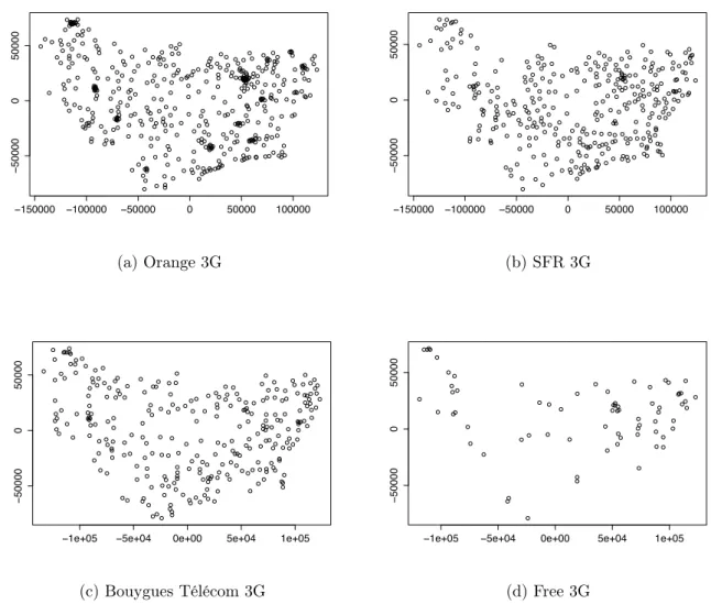
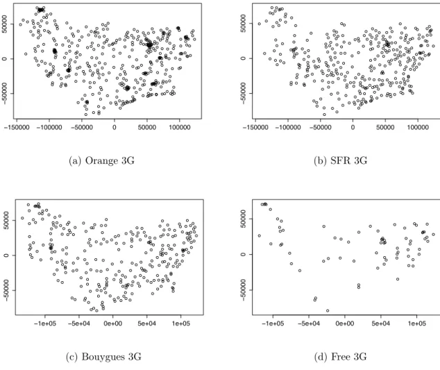
The performance of a cellular network is strongly linked to the spatial repartition of its agents (base stations and users). On the downlink, the spatial repartition of the antennas plays a major role. Localization of the base stations are indeed random, however, this randomness is tied by externalities and engineering choices such as the density and the spatial repartition of users to serve, the locations that are available to set up an antenna, and the overall interference in the network. −150000 −100000 −50000 0 50000 100000 − 50000 0 50000 (a) Orange 3G −150000 −100000 −50000 0 50000 100000 − 50000 0 50000 (b) SFR 3G

−1e+05 −5e+04 0e+00 5e+04 1e+05

−

50000

0

50000

(c) Bouygues Télécom 3G

−1e+05 −5e+04 0e+00 5e+04 1e+05

−

50000

0

50000

(d) Free 3G

Figure 1.1: 3G deployment for rural areas for the Haute-Saône, la Haute-Marne and Vosges perfectures, France for the four operators (distances are in meters).

On a macroscopic (regional) scale, it is obvious that cells are placed not only along com-munications routes such as freeways and roads, but also in villages and local cities. Figure 1.1 gives an insight on how antennas are placed in a rural region. Coverage is the main issue,

(12)

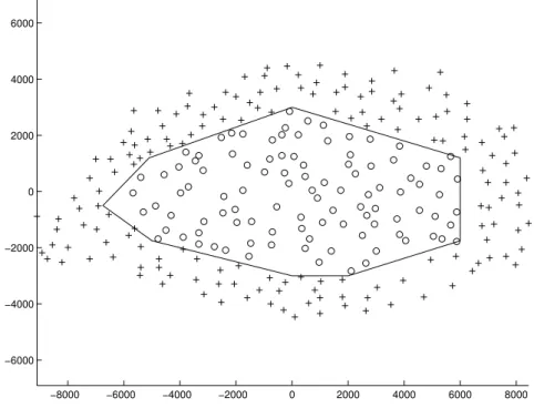
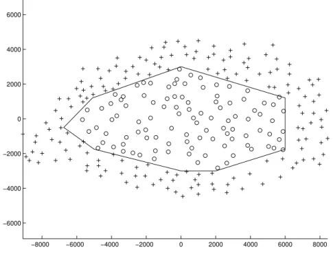
therefore cells are placed far from one another to maximize their footprint. Cities, on the other hand concentrate users on a small area. If antennas are still placed along streets, they are regularly spread in the city in order to limit the interference with one another. In this situation, signal degradation due to inter-cell interference is a real challenge that has to be traded-oﬀ with the local increase in the density of antenna on hot-spots, aimed at fulfilling local capacity needs. Figure 1.2, that gives the deployment in Paris for the operator SFR, illustrates this phenomenon.

−8000 −6000 −4000 −2000 0 2000 4000 6000 8000 −6000 −4000 −2000 0 2000 4000 6000

Figure 1.2: SFR UMTS 900 MHz network deployment over Paris (distance in meters). Network models that describe the locations of the base stations are based on point pro-cesses. Base stations are placed as points in a plane. The law of the underlying point process provides statistical properties that can be linked with the overall network performance. The mostly used and widespread model that is considered in many research papers and models is the hexagonal grid. The honeycomb conjecture indeed states that the hexagonal shape is the best way to divide a surface into regions of equal area with the least total perimeter. This theorem embodies the antagonist forces that leads network deployment engineering (the trade-oﬀ between signal quality and inter-cell interference) to its deterministic ideal. Although this model is an easy way to conceive and use in numerical simulations, general results on networks are complex to obtain theoretically [69]. Even the honeycomb conjecture itself has only been proven in 1999 [55].

The Poisson point process that has been introduced for cellular network applications by Baccelli et al. [6], constitutes the stochastic counterpart of the hexagonal model. Closer to the inherent reality of deployed networks, it introduces a wide range of mathematical tools to understand cellular networks. A homogeneous Poisson point process is easy to simulate: let Abe a compact in the plane and |A| is area. We designate by > 0 the density of points per

(13)

−0.4 −0.2 0 0.2 0.4 0.6 −0.5 −0.4 −0.3 −0.2 −0.1 0 0.1 0.2 0.3 0.4 0.5

Figure 1.3: Realization of a Poisson point process.

unit of surface. The number of points to be drawn in the plane is given by a Poisson law with intensity |A|. Points are drawn uniformly and independently in the chosen compact. Figure 1.3 gives a realization of a Poisson point process. The property that points are independent between one another, provides the Poisson point process its tractable mathematical properties. It is also because of this very property that the Poisson point process lacks realism. Since there is no dependency between points, a repulsive force between them does not exist. Therefore, cluster of points can occur with high probability, which is sub-optimal in terms of inter-cell interference and does not comply with the fact that while engineering a cellular network, one must place antennas in order to maximize their coverage while fulfilling traﬃc needs. Hence, An underlying dependency between the positions of the base stations must exist, even though it is in a less rigid way than in the hexagonal model.

Using the Poisson point process as a base process, one can derive new point processes where clusters of points are avoided. For example, Mattern hard core type I and II point processes have been studied [47]. For a type I Mattern hard core point process, a distance d is considered. Then, for each point of a given Poisson point process realization, the point is kept if there is no other point at a distance smaller than d. For type II Mattern hard core point process, a random mark is associated with each point, and a point of the parent Poisson point process is deleted if another point exists within the hard-core distance d with a smaller mark. Such kind of transformation based on an exclusion area qualifies the resulting point processes as hard core. Since the points near one another are removed during the thinning, the resulting realization does not contain clusters of points. However, even if realizations of Mattern hard core Type I and II point processes are easily computed, theoretical results are proven to be complex to derive.

Another candidate family of point processes, the ↵-stable point processes, has been fitted on Chinese [85] and European networks [19] and some conclusions about network exploitation

(14)

costs have been derived. Comparative studies between point processes also exist [86, 20]. Point processes have also a wide range of applications, one of which is quantum physics. The determinantal point process family that was introduced by Shirai et al. [76]. Among them, the Ginibre point process models positions of the electrons trapped in space. Since electrons possess a negative electric charge, their positions in the plane is the result of the equilibrium between the trap and the particle repulsive interaction. These two antagonist eﬀects are analogous to the ones that drive the deployment of networks. And since many theoretical results are available [52, 14, 57, 15, 51, 75], the Ginibre point process model was later introduced to describe wireless networks [68]. This model on the contrary of the Poisson point process introduces too much dependency between points. Clusters of points that might exist in real deployment occur empirically with a higher probability than in a realization of a Ginibre point process but with lower probability than in a Poisson process.

The -Ginibre model fills that middle ground between the Ginibre point process and the Poisson point process. A realization of a -Ginibre point process can be obtained from a realization of a Ginibre process. A thinning is performed on the parent Ginibre point process such that each point is kept independently from each other with a probability . A re-scaling with parameterp is performed to preserve the intensity. If is equal to one, the resulting point process is a Ginibre point process. For decreasing, each point is kept with smaller and smaller probability. Therefore, neighbor dependency between points tends to disappear. The resulting point process thus tends to a Poisson process. Figure 1.4 gives three realizations for three diﬀerent values of .

The flexibility of the -Ginibre model along with an existing mathematical literature [76, 68, 39, 43, 42, 51, 56, 31, 24, 41, 78, 64] make it an interesting candidate to describe wireless networks with finesse. Only two parameters are required: that rules the equilibrium between repulsiveness and local densification, and the intensity which can be linked to the underlying traﬃc. Many theoretical results were derived especially on signal quality in wireless networks. In this dissertation, the relevance of the -Ginibre is first discussed. Thanks to Cartoradio [4] and the ANFR (French national electromagnetic spectrum regulator), positions of base stations are made available to the general public. This data is accurate since it is mandatory for any French operator to declare the positions of their operational base stations. A fitting is performed on data collected on several environments (dense urban area (Paris), suburban and rural areas) and on each technology. Couples of values ( , ) are deduced for each network. By comparing the relative values of the couples, conclusions are drawn on the deployment strategies of each network. The superposition of all the antennas deployed by every operators is also analyzed. We show that on a global scale, the Poisson point process model still holds for superpositions, confirming the theorem on the superposition of realization of independent

-Ginibre point processes [44].

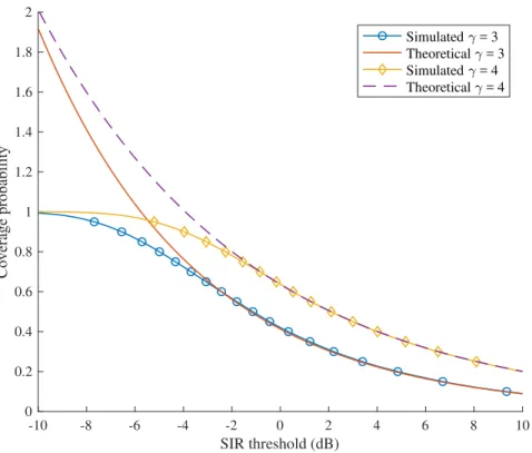
The parameter gives also insights on the overall signal quality in the network. Indeed, for a given threshold ✓ > 0, there is a dependence between the coverage probability P (SINR > ✓) and the parameter . The limit capacity on a point to point link defined by Shannon is a function of the bandwidth and also of the SINR at the point of the network considered. Since the SINR and the demand for traﬃc (for instance from users in the network) are constraints that are diﬃcult to adjust in real time, it is spectrum that is dynamically allocated to users to fulfill their needs. For instance, in LTE networks, the number of resource blocks allocated to a given user in a sub-frame defines the throughput on the link. A dependence thus exists between the parameter and the point to point capacity and consequently on the number of resource blocks allocated to users during a sub-frame. As the number of resource blocks are

(15)

−0.4 −0.2 0 0.2 0.4 0.6 −0.5 −0.4 −0.3 −0.2 −0.1 0 0.1 0.2 0.3 0.4 0.5 (a)1_/₄-Ginibre −0.4 −0.2 0 0.2 0.4 0.6 −0.5 −0.4 −0.3 −0.2 −0.1 0 0.1 0.2 0.3 0.4 0.5 (b)1_/₂-Ginibre −0.4 −0.2 0 0.2 0.4 0.6 −0.5 −0.4 −0.3 −0.2 −0.1 0 0.1 0.2 0.3 0.4 0.5 (c)3_/₄-Ginibre

Figure 1.4: Examples of -Ginibre point process realizations.

in a limited number, the parameter influences therefore network performance and capacity. While most of the works tend to characterize only the signal quality in the network [46, 40], we analyze the influence of the parameter on the overall resources and potential throughput of the network. Since the simulations must take place in a reference cell (typically a cell that is placed in the middle of the network), we introduce a new simulation scheme to obtain realizations of -Ginibre with a point at the origin of the plane. In this cell, the outage probability is taken as our main metric to understand the eﬀects of spatial repartition on the overall performance of the network. We also provide tools to estimate the best dimensioning strategy provided a given outage probability and a couple ( , ).

1.2.2 Resource allocation and optimal transport

In this dissertation, we also consider a method allocate resources in downlink. In order to increase the overall throughput of the network, we consider that base stations cooperate with one another. In the case of an OFDMA network, a user can then receive resource blocks from multiple base stations. One has then to know which resource block is allocated to which user from which base station. That is what we call the routing problem. We focus on a

(16)

novel approach that jointly optimizes bandwidth allocation and resource routing in OFDMA networks. The originality of this framework lies in the fact that the analysis is performed on rough assumptions (only the SINR of the link is required) and that performance analysis takes into account the influence of the -parameter. On a theoretical point of view, we propose an original quadratic formulation of the resource allocation problem. We aim at finding the optimal coupling that links the supply of network resource and the traﬃc demand. Since the coupling also shapes the quantity of resource that is allocated to each user, this problem is solved thanks to optimal transport theory and Cournot-Nash equilibria.

The Cournot-Nash equilibria was first introduced by Antoine Augustin Cournot in 1838, to model the supply and demand of bottled water companies. This market being a duopoly implied that slight modifications of the supply had consequences on the structure of the demand, as well as the repartition of the market shares. The Cournot model highlights the equilibria points (that were proven to be a subset of Nash equilibria [66]) where the market was the most eﬃcient [23, 79]. Blanchet et al. have recently investigated the Cournot-Nash equilibria [11, 8, 9] under a modern formulation introduced by Mas-Collel [62]. Methods to reach the equilibria solutions are also discussed [10, 12, 81]. The originality of their approach is to formulate the Cournot-Nash equilibria under the light of Optimal transport thanks to the coupling that exists between supply and demand.

Optimal transport has been introduced by Monge in 1781 [65]. The formulation of the problem is simple: given that there is a pile of sand and a hole in the ground, what is the path that each grain of sand must follow in order to minimize the energy to transfer the pile into the hole? This problem was solved by Kantorovich [54] during World War II. Optimal transport is nowadays widely applied in imaging to synthesize images and textures [73, 71, 72, 35] and has been recently widely developed on a mathematical point of view by numerous works [25, 58] and by Villani [80]. In the field of wireless networks, Optimal transport has been applied to find the position of base stations placed in floating air balloons considering the user repartition [67] and to solve traﬃc congestion [77].

1.3 Outline

This dissertation is organized in four parts: Chapter 2 gives the mathematical tools to manip-ulate the point processes, Chapter 3 overviews the relevance of the -Ginibre model on real data and introduces the convergence theorem for a superposition of -Ginibre. In Chapter 4, the link between the parameter and the performance of the network is described for networks based on resource block allocation. In Chapter 5, a general performance analysis scheme is in-troduced thanks to Optimal transport and the Cournot-Nash equilibium framework. Finally, we conclude in Chapter 6.

(17)

(18)

Point processes

Stochastic geometry and more precisely random point processes have raised interest in the wireless network community. Point processes are used to model the positions of the base stations or users in the plane. Two models have gained popularity thanks to their mathematical properties as well as practical characteristics: the Poisson point process [6] and the -Ginibre point process [63]. Far from excluding one another, they are strongly bounded by several convergence theorems [31]. In this chapter, we introduce the formal definitions of the Poisson point process and the -Ginibre point process. Numerous tools to analyze and characterize point processes such as the summary statistics and the Palm measure are also introduced. Finally, a novel theorem on the superposition of realizations of -Ginibre point processes is exposed as well as a novel simulation framework to obtain realizations of -Ginibre point processes under the Palm measure.

2.1 Introduction to point process theory

In this section, we provide definitions and notations to formally define point processes and give their main characteristics.

2.1.1 Configuration space and point processes

Let E be an Euclidian space such as R2 _{or C. We first introduce the notions of configuration}

and configuration space.

Definition 2.1 (Configuration). A configuration, denoted , is a finite or countable-infinite collection of points, without accumulation.

Hence a configuration is a set of points = {x1, x2, . . .}, with each xi 2 E. The

non-accumulation property means that the number of points in any bounded subset A ⇢ E is finite. For instance, the set of points {z = 1/n | n 2 N⇤_{} is not a configuration since 0 is an}

accumulation point. Indeed, the number of points in the unit ball is infinite.

We denote the number of points of a configuration in the subset A ⇢ E by (A). A way to calculate the quantity (A) is given by

(A) =X

x2

x(A),

(19)

where x is the Dirac measure on A such that x(A) = 1 if x lies in A, and x(A) = 0

otherwise. Thanks to the Dirac measure, we are able to compute functions defined on E with configuration of points such that for all functions f defined on E, we have:

Z

E

f (x) (dx) =X

x2

f (x).

Definition 2.2(Configuration space NE). The configuration space NE is the space of all the

configurations on E.

We now introduce the definition of point processes that stochastic processes: Definition 2.3 (Point process). A point process is an NE-valued random variable.

An outcome of a point process is also called a realization. Since a point process is a random variable on the configuration space NE, its law is denoted by:

8 2 NE, P ( ) = P( = ). (2.1)

In other terms, if F is the Borel -algebra on NE, and P the law of , the point process

is a canonical random variable on (NE,F, P ).

Characterizing a point process with its law is often diﬃcult in practice, since direct cal-culation on NE is not convenient. The Laplace transform fully defines a point process and

allows calculations on the usual space E.

Definition 2.4 (Laplace transform). The Laplace transform of a point process is defined for all continuous non-negative function f on E such that

L (f) = E he REf (x) (dx) i , =E he Px2 f (x) i , = Z NE e Px2 f (x)_dP ( ).

2.1.2 The Poisson point process

The Poisson point process can be defined by its Laplace transform.

Definition 2.5(Laplace transform of the Poisson point process). Let ⇤ be a measure. For all continuous function f on E, the Laplace transform of the Poisson point process P is given

by

L P(f ) = e R

E(1 e f (x))⇤(dx).

For instance, the measure ⇤ is often the intensity measure ⇤(dx) = dx, with > 0 and dx being the Lebesgue measure. In this document, we will only consider the homogeneous Poisson point process. Therefore, we always assume that ⇤(dx) = dx.

Thanks to the Laplace transform of a Poisson point process, we can derive the Campbell formula:

(20)

Theorem 2.1(Campbell formula [70]). For all function f 2 L1_{(E, ⇤)}_{, the space of ⇤-measure}

integrable functions, and P a Poisson point process,

E P Z E f (x)d (x) = Z E f (x)d⇤(x).

While the Laplace transform comprehensively characterizes the law of a point process in a calculation point of view, it does not provide an intuitive definition of it.

For instance, an alternate and more common definition of the Poisson point process is the following:

Definition 2.6 (Poisson point process). Let ⇤ be a measure. The point process P is a

Poisson point process, if and only if

P { P(A1) = n1, . . . , P(Ak) = nk} = k Y i=1 e ⇤(Ai)⇤(Ai) ni ni! , for every k 2 N⇤_{, n}

1, . . . nk2 N and all bounded mutually disjoint subsets of E: A1, . . . , Ak.

The Poisson distribution can be easily recognized in the previous definition. Furthermore, the number of points of a Poisson point process is deduced in the following proposition. Proposition 2.1. For all compact A ⇢ E, we have

P ( (A) = n) = (⇤(A))_n! ne ⇤(A).

2.1.3 Operations and properties on point processes

Point processes are stochastic processes, thus notions of stationarity, ergodicity and conver-gence in law can be defined.

Definition 2.7 (Stationarity). Let be a point process and =_{xi}i2N be a realization of

. For all t 2 E, we denote by + t the point process with realization + t = {xi+ t}i2N.

The point process is stationary if and only if and + t have the same law.

Definition 2.8 (Ergodicity). Let be a point process and be a realization of . A point process is ergodic if for any family of subsets {An} n 2 N, such that A1 ⇢ A2 ⇢ . . . ⇢ E,

and for any function f : E ⇥ NE ! E, the following limits exist and verify:

lim n!1 1 |An| Z An f (t, t)dt = lim n!1 1 (An) Z An f (t, t) (dt)

The left hand side of the equation is to the mean of f on E, while the right hand side is the mean of f on the realization of the point process.

Definition 2.9 (Convergence in law). Let { n}n2N be a family of point processes, and a

point process. The family { n}n2N converges in law towards , written n n!1! , if for all

bounded continuous function f : NE ! R, we have:

lim n!1E n[f ] =E [f] , nlim!1 Z NE f ( )dP _n( ) = Z NE f ( )dP ( ).

(21)

Point processes are also configurations, thus notions of scaling, superposition and indepen-dent thinning can be defined.

Definition 2.10 (Scaling). Let be a point process and one of its realization. Let s > 0. We denote by sthe point process with realization s=Px2 sx. Then, the point process s

is a scaling of .

Definition 2.11 (Superposition). Let and be two point processes and and be one of their realizations. The point process + with realization + , which is the union of the two sets of points and , is the superposition of and .

The reverse operation is the superposition is called a thinning.

Definition 2.12 (Independent thinning). Let be a point process and one of its realiza-tion. Let (Ux, x2 ) be a family of {0, 1}-valued independent and identically distributed (i.i.d)

random variables, independent of the realization , with p(x) = P(Ux= 1). The point process

with realization =P_x2 Ux x is an independent thinning of with probability p.

Points of the thinning of a realization are selected independently from one another. The Poisson point process illustrates the previous definitions with the following properties: Proposition 2.2 (Properties of the Poisson point process [70]).

• The homogeneous Poisson point process is stationary and ergodic.

• An independent thinning of a Poisson point process of parameter ⇤ with probability p is a Poisson point process with intensity p⇤.

• A superposition of several independent Poisson point processes is also a Poisson point process whose intensity is the sum of the underlying point processes intensities.

2.1.4 Correlation functions and Palm measure

Point processes can also be defined thanks to their correlation functions.

Definition 2.13 (Correlation functions). Let be a point process and ⇤ be a measure on E. The correlation functions of in respect to the measure ⇤, denoted ⇢k : NE ! R for

k2 N⇤_{, are given by:}

E " _k Y i=1 (Bi) # = Z B1⇥...⇥Bk ⇢k(x1, . . . , xk)⇤(dx1) . . . ⇤(dxk), (2.2)

for any family of mutually disjoint compact B1, . . . Bk ⇢ E.

For any finite configuration {x1, . . . xk}, the k-th correlation function ⇢k(x1, . . . xk) of a

point process is the probability to have exactly k points in the vicinity of each one of the {x1, . . . xk}.

For instance, the correlation functions of a Poisson point process of intensity , where ⇤(dx) = dxare computed thanks to Equation (2.2). Using previous notations, since Poisson point processes on disjoint sets are independent,

E " _k Y i=1 (Bi) # = k Y i=1 E [ (Bi)] .

(22)

Thanks to the Campbell formula, E " _k Y i=1 (Bi) # = k k Y i=1 |Bi| = Z B1⇥...⇥Bk dx1. . . dxk.

Therefore, by identification with Equation (2.2), the correlation functions of the Poisson point process are for any k 2 N⇤

⇢k(x1, . . . , xk) = 1.

The correlation functions can indicate the repulsiveness or attractiveness of a point process. Definition 2.14 (Repulsive and attractive point process). A point process with correlation functions ⇢k, for k 2 N⇤, is repulsive (resp. attractive) if for x, y in E, we have :

⇢2(x, y) ⇢1(x)⇢1(y) (resp. ⇢2(x, y) ⇢1(x)⇢1(y))

From the correlation functions, we can derive the following definition of the Palm measure. Definition 2.15 (Palm measure [21]). Let be a point process with correlation functions (⇢k, k 1). The Palm measure of is the law of the point process whose correlations functions

are given by

⇢0_k(x1, . . . , xk) =

⇢k(x1, . . . , xk)

⇢1(0)

.

The Palm measure can be interpreted as the distribution of given that ({0}) = 1. Since its correlation functions are all equal to 1, the Palm measure of a Poisson point process is given by the following proposition.

Theorem 2.2 (Slivnyak-Mecke Theorem). The Palm measure of a Poisson point process is its own law. As a result, to obtain a realization of a Poisson point process under the Palm measure, it suﬃces to add the point {0}.

2.2 Point process characterization via statistical inference

Statistical inference is performed thanks to summary statistics functions that are defined below. They are used to infer properties and characterize a point process from the observation of its realizations. One can remark that, when studying a given realization, properties may diﬀer given the point of view of the observer. We provide a short example below.

Let be a configuration of points of integer coordinates = {(i, j)}(i,j)2Z2, as represented

on Figure 2.1.

Let us consider z a point in C. We denote by d( , z) the distance between the nearest point of the configuration that is not z and the point z. Considering the infinity norm k k1,

d( , z) = min x2 x6=z kz x_k₁, d( , z) = min x2 x6=z max(_<(z x),_=(z x)).

(23)

x y

(1, 1) 0

Figure 2.1: Configuration = {(i, j)}(i,j)2Z2

If z is in C, d( , z) > 0 and depends of the position of z. Meanwhile, if z is in , d( , z) = 1. Hence, interpretations of the properties of a configuration may diﬀer according to the point of view from which is observed. Therefore we consider the following summary statistic functions:

Definition 2.16(Contact distribution function F [64]). Let be a realization of a stationary point process . The contact distribution is the probability that for any point x of E, no point lies in an open ball of center x and radius r, denoted b(x, r). For r > 0,

F (r) =P ( (b(x, r))>0) .

Since the point process is stationary, we can choose x to be o = (0, 0). Example: For the Poisson point process of intensity , we have for all r > 0:

F (r) = 1 e ⇡r2.

Definition 2.17 (Nearest neighbor distance distribution function G [64]). Let be a real-ization of a stationary point process . For x in , we denote by x the point process with

realization \ {x}. The nearest neighbor distance distribution is the probability that for any point x of , no other point lies in an open ball of center x and radius r. For r > 0,

G (r) =_{P (} x(b(x, r)) > 0) .

Example: For the Poisson point process of intensity , we have for all r > 0: G (r) = 1 e ⇡r2.

Definition 2.18 (J Function [64]). Let be a realization of a stationary point process. The J function is the ratio for all r > 0:

J (r) = 1 G(r) 1 F (r)

(24)

Example: For the Poisson point process, the J function is equal to 1 for all r > 0, by definition.

Proposition 2.3.If J(r) 1(resp. J(r)  1) for all r > 0, then the point process is repulsive (resp. attractive).

Indeed for a given point process, if J is bigger than 1, then the G function is smaller than the F function. This means that the probability that a point of the point process lies at a distance from a point x smaller than r > 0, is smaller when x is part of the process than when x is any point in the plane. Therefore the nearest neighbor is closer if the observer is not in the configuration.

2.3 The -Ginibre point process

2.3.1 Definition and properties

We now introduce the definition of kernel and determinantal process required to build the -Ginibre point process.

First, let ⇤ be a measure on C. Let us consider the square integrable complex functions space L2₍_{C, ⇤), equipped with the Hilbert scalar product defined for any f and g in L}2_{(A, ⇤)}

on a compact set A ⇢ C:

f· g = Z

A

f (x)g(x)⇤(dx), with z being the conjugate complex of z 2 C.

A kernel K is a measurable function from C2 _{to C.}

Definition 2.19 (Locally square integrable kernel). A kernel K is locally square integrable if for any compact set A ⇢ C, we have

Z

A|K(x, y)|

2_{⇤(dx)⇤(dy) <}_1.

Definition 2.20 (Hermitian symmetric kernel). A kernel K is Hermitian symmetric if K(x, y) = K(y, x).

Theorem 2.3 (Spectral theorem). If the kernel K is Hermitian symmetric, there exists an orthogonal basis K

n n2N on L2(A, ⇤), with A compact subset of C, with corresponding

eigen-values K

n n2N such that for all (x, y) 2 A2,

K(x, y) = 1 X n=0 K n Kn(x) Kn(y).

Definition 2.21 (Trace-class kernel). A kernel K is trace-class if its eigenvalues verify K(x, y) =

1

X

n=0

| Kn| < 1.

(25)

Definition 2.22 (Determinantal point process). Let K be a bounded, Hermitian symmetric, locally trace-class kernel on L2_{(A, ⇤)}_{, with A compact subset of C, such that its eigenvalues}

verify K

n < 1 for all n 2 N. For any k-tuple of points {x1, . . . , xk} 2 Ak, a determinantal

point process is a point process with correlation functions such that: ⇢k(x1, . . . , xk) = det (K(xi, xj)1i,jk) ,

where det (K(xi, xy)1i,jk) is the determinant of the matrix of which the element of the i-th

row and j-th column is K(xi, xj).

Proposition 2.4 (Laplace transform of a determinantal process). The Laplace transform of a determinantal point process is given for all non negative functions f by

L (f) = Det(I + Kf), where Kf(x, y) = ⇣ 1 e f (x)⌘1/2K(x, y)⇣1 e f (y)⌘1/2, and Det(I + Kf) = 1 X n=0 1 n! Z En det ( K(xi, xj)1i,jn)dx1. . . dxn

which is called the Fredholm determinant.

The determinantal point process is a repulsive point process, since its correlation functions verify

⇢k(x1, . . . xk) ⇢1(x1) . . . ⇢k(xk).

Hence, the probability to find k points of the point process in the neighborhood of {x1, . . . , xk}

is smaller than the probability to find a point of the point process near each one of the {x1, . . . , xk}.

There are numerous kernels of determinantal point processes. The -Ginibre point process is a specific determinantal point process.

Definition 2.23 ( -Ginibre point process). Let > 0 and _{2 ]0, 1]. The -Ginibre point} process is the determinantal point process with kernel

K , (x, y) = e ⇡

2 (|x|2+|y|2 2xy)_, (2.3)

is then called the intensity of the point process.

If = 1, the point process is called the Ginibre point process and has for kernel

K (x, y) = e 2⇡(|x|2+|y|2 2xy). (2.4)

We introduce now a well-known result.

Lemma 2.1 ([31]). When goes to zero, the -Ginibre of intensity converges in law to a Poisson point process of the same intensity.

(26)

Proof. We provide here an informal proof, a full proof can be found in [31]. We have that for all (x, y) 2 C,

lim

!0K , (x, y) = x(y).

We denote this limit by K0, and we can see that it is a diagonal matrix with as diagonal

coeﬃcients. Therefore the Laplace transform of the resulting point process is for any non negative f L (f) = 1 X n=0 1 n! Z Cn det⇣ (1 e f (xi)₎1/2_K 0, (xi, xj)(1 e f (xj))1/2 ⌘ 1i,jndx1. . . dxn = 1 X n=0 1 n! Z C(1 e f (x)₎n₍ ₎n_dx = e RC(1 e f (x)) dx.

We recognize the Laplace transform of a Poisson point process.

Therefore, the coeﬃcient can be seen as a repulsive factor: the greater the coeﬃcient is , the more repulsive the -Ginibre point process is. Since the kernel K , is Hermitian

symmetric, the spectral theorem can be applied to any -Ginibre point process kernels. Theorem 2.4. The eigenvalues of the kernel of a -Ginibre point process restrained on the ball C = b(o, R), for R > 0, is given by

K , (x, y) = X n 0 , n n, (x) n, (y), with , n = ˜ n + 1, ⇡R2_/ n! , and , n = s ˜(n + 1, ⇡R2_{/ )}e ⇡ 2 |z|2 s ⇡ z !n , where ˜ is the lower Gamma function defined by for all z 2 C and a 0:

˜(z, a) = Z a

0

e ttz 1dt,

Proof. Let ( ,

n )n2N be the family on L2(C, dz) such that for all complex z 2 C:

, n (z) = r n!e ⇡ 2 |z|2 s ⇡ z !n . (2.5)

(27)

Combining Equation (2.3) and Equation (2.5), the kernel K , is K , (x, y) = e ⇡ 2 (|x|2+|y|2 2xy) = e ⇡(xy)e 2⇡(|x|2+|y|2) = X n 0 1 n! ✓ ⇡ xy ◆n e 2⇡(x2+y2) =X n 0 , n (x) n, (y). The family ( ,

n )n2N is an orthogonal family of L2(C, dz). Therefore, each vector has to

be normalized to obtain an orthonormal family. The norm of , n is : k n,k2= Z C , n (z) n, (z)dz = Z Cn! e ⇡|z|2 ✓ ⇡◆n |z|2ndz = n! ✓ ⇡◆n✓Z R 0 e ⇡r2r2n+1dr ◆ ✓Z ⇡ ⇡ d✓ ◆ = n! Z ⇡R2_/ 0 e ttndt = ˜ n + 1, ⇡R 2_/ n! .

By identification with the spectral decomposition, we have that for any n in N

, n = , n k n, k and _n, =_k_n, _k2.

According to Proposition 2.2, the superposition of independent Poisson point process is Poisson point process. For the superposition of -Ginibre point processes, we introduce the following theorem :

Theorem 2.5 ( -Ginibre point process superposition convergence theorem [44]). For all n_{2 N}⇤, let n be the superposition of n independent n,i-Ginibre point processes { n,i} with

intensities n,i= i/n and n,i2]0, 1], for 1  i  n. Let us suppose that:

(i) the sequence ( i)i2N⇤ ⇢ R⇤₊ is bounded,

(ii) lim n!+1 1 n Pn i=1 i = .

Then ( n)n2N⇤ converges in law to a Poisson point process with intensity .

Proof. Theorem 2.5 is achieved if all conditions of Theorem 2.6 are satisfied. Let A be a compact subset of C.

(28)

Theorem 2.6. [Convergence in law theorem [53]] For any A compact subset in C, if the three following properties hold:

(i) lim

n!+1P( n(A) = 0) =P( (A) = 0)

(ii) lim sup

n!+1 P( n(A) 1) P( (A)  1)

(iii) lim

t!+1 lim supn!+1 P( n(A) > t) = 0

Then: n n!1! .

Proof of Condition (iii) By definition of the expectation, P( n(A) > t) E[ n

(A)]

t .

Since (E[ n(A)])_n2N is bounded, (iii) holds.

Proof of condition (i) and (ii) For a Poisson point process, we know that: P ( (A)=0)=e |A| ⇡ 1

, P ( (A)1)=e |A| ⇡ 1

1+|A| ⇡ 1 .

We have to calculate yet the left-hand side of both inequalities (i) and (ii). Let Kn,i be the

kernel of a n,i-Ginibre point process. Proposition 3 of Goldman’s paper [43] states that:

P( n,i(A) = 0) = 1+ X p 1 ( 1)p p Z Ap det[Kn,i](x1, ..., xp)dx1. . . dxn,

P( n,i(A) = 1) =P( n,i(A) = 0)

Z A Rn,i(z)dz. with Rn,i(z) = Kn,i(z, z)+ X j 2 K_n,i(j)(z, z).

By hypothesis of Theorem 2.5, ( i)i2N⇤ is bounded. We also know that kKn,ik1 = ci(n⇡) 1.

We can then prove recursively for all p 1, that there exists M > 0 such that for all i 2 N⇤, 0 det[Kn,i](v1, ..., vp) kKn,ikp₁

✓ M n⇡

◆p

.

Therefore, the two bounded sequences (✏n)n2N⇤ and (✏0_n)_n2N⇤independent of i exist and verify:

P( n,i(A) = 0) = 1 i|A|

n +n

2_✏ n.,

P( n,i(A) = 1) = i|A|

n +n

2_✏0 n.

(29)

Hence, P( n(A) = 0) = eO(n 2₎ e Pni=1 i|A|n , P( n(A) = 1) eo( 1 n)e Pn j=1 j |A| n n X i=1 i|A| n + o(1). Therefore, lim n!1P( n(A) = 0) = e |A| _, lim sup n!1 P( n(A) = 1) |A|e |A| _,

consequently (i) and (ii) hold.

Hypotheses (i) and (ii) of Theorem 2.5 are quite restrictive since the intensities of each -Ginibre point process are dependent of n. However, here, we mainly work with finite families of -Ginibre point process. Therefore, we can choose the value of the ( i)i21...n such that

they equal the intensities of the -Ginibre point processes that are superposed. This result about superposition of the -Ginibre is completed by the works of Decreusefond et al. [31] that explore in details the asymptotic behavior of point processes superposition.

2.3.2 The F , G and J functions for the -Ginibre point process

We here give the value of the summary statics functions defined in Paragraph 2.2 for a -Ginibre point process.

Proposition 2.5(The F function for the -Ginibre point process [33]). For all r > 0, the F function of the -Ginibre point process is

F (r) = 1 1 Y k=1 0 @1 ˜ ⇣ k, ⇡r2⌘ (k 1)! 1 A .

Proposition 2.6(The G function for the -Ginibre point process [33]). For all r > 0, the G function for the -Ginibre point process is

G (r) = 1 1 Y k=2 0 @1 ˜ ⇣ k, ⇡r2⌘ (k 1)! 1 A .

Proposition 2.7 (The J function for the -Ginibre point process[33]). For all r > 0, the J function for the -Ginibre point process is

J (r) =⇣1 + e ⇡r2⌘ 1. Proofs of these propositions can be found in [33].

(30)

2.3.3 Simulation of a -Ginibre under the Palm measure

The most simple way to simulate a -Ginibre of intensity is the following [42]: • Draw N2 _{i.i.d random complex coeﬃcients m}

i,j such that mi,j ⇠ N (0, 1) + iN (0, 1),

with N (0, 1) be a normal distributed random value. • Compute the eigenvalues of M = (mi,j)1i,jN.

• Perform an independent thinning of parameter on the eigenvalues of M. The resulting set is denoted .

• Perform a scaling of parameterp ⇡ on .

Even if this algorithm is eﬃcient in terms of complexity and time, there are many drawbacks to be considered.

The first one is the fact that this algorithm simulates a -Ginibre with a truncated kernel defined for all (x, y) 2 C2_,

K(x, y) = N 1_X n=0 , n (x) n, (y), as showed in [39].

The second drawback comes from the fact that one has no control on the size of the simulation domain.

The third drawback comes from the fact that it is not possible to simulate realizations of a -Ginibre point process under the Palm measure. For instance, if is a realization of a point process , and x1 the point of that is the nearest to the origin, a naive approach would be

to consider the realization x1, which is the translation of by a vector x1. However, this

method is not correct. Let us consider the law of the aﬃxes of the points of the realization of a -Ginibre point process.

Lemma 2.2([52, 56]). Let be a -Ginibre point process and {Gj,k}_j,k2N be i.i.d exponential

random variable of parameter one, we define Xj law= v u u t ⇡Xi k=1 Gj,k.

Then, the law of the aﬃxes of is the same as the law of the set of {Xj}_j_2N on which a

thinning of probability has been performed.

Figure 2.2 illustrates the probability law of the event Xj < X1 for j > 1, computed for the

Ginibre point process. It appears that choosing the point nearest to the origin leads to select a point with an aﬃx following the law of some Xj instead of X1 with about 50% probability.

Therefore, statistical bias is introduced.

As a consequence, in order to simulate a -Ginibre under the Palm measure, we adapt the framework presented in the works of Flint [39] and Decreusefond et al. [28], that is used to simulate realizations of Ginibre point process. This framework is itself derived from Algorithm 18 of the works of Hough et al.[51], which provides a method to simulate realizations of a determinantal point process provided its kernel eigenvectors and eigenvalues.

(31)

j=2 j=3 j=4 j=5 j=6 j=7 j=8 Prob(Xj < X1) 0.00 0.05 0.10 0.15 0.20 0.25

Figure 2.2: Probability P (Xj > X1) for a Ginibre point process of intensity

The following theorem which can be found in [51], provides us with the first milestone to construct a realization of a -Ginibre point process. Let us denote by B( ) the 0/1-Bernoulli random variable of parameter .

Theorem 2.7 ([51]). The number of point of a -Ginibre point process on a ball C has the the distribution ofP1

n=0B( n, ) where (B( n, ), i 0)is a family of independent Bernoulli

random variables. In particular,

E [ (C)] = 1 X n=0 , n = ⇡R2. Moreover, let I ={n 0, B( _n, ) = 1}, and K_I, (x, y) =X n2I , n (x) n, (y).

Then, given I, a realization of on a ball C has |I| points and the joint distribution of the locations of these points is given by

p(X1 = x1, . . . , X_|I| = x_|I|) =

1

|I|!det K

I

, (xi, xj), 1 i, j  |I| . (2.6)

According to Theorem 2.7, a realization of a -Ginibre of parameter c is build in two times: the first step is to draw the Bernoulli random values in order to get the number of points |I| of the realization and construct the kernel K ,

I . Provided these two pieces of information,

(32)

Let M be the maximum number of points that can be drawn for a given realization of a -Ginibre point process of parameter :

M = sup

n {n, B( ,

n ) = 1}.

Since the random variables B( ,

n )are independent random variable, the law of M is:

P(M < k) =Y1 i=k (1 _i, ) and P(M = k) = _k, 1 Y i=k+1 (1 _i, ). (2.7)

We also know that since the outcome M = k only depends on the set of random variables (B( _i, ), i k),

P⇣B( _i, ) = 1 M = k⌘= _i, .

Algorithm 3 provides the method to draw the number of points M and compute the kernel KI_, .

Data: ( , n ).

Result: KI , , M.

Let M be drawn according to (2.7); for n from 1 to M do if B( , n ) = 1then KI_, (x, y) = KI_, (x, y) + n, (x) n, (y) end end

Algorithm 1:Determination of the maximum number of points M and construction of the kernel KI

, .

Once the maximum number of points M fixed and the kernel KI

, constructed, we can

now draw the points in the ball C. Each point of a realization is computed iteratively. Indeed, considering the joint-density p(x1, . . . x|I|) as the product of conditional probabilities:

p(X1= x1, . . . , X_|I| = x_|I|) = p(X1 = x1) . . . p(X_|I|= x_|I||x1. . . X_{|I| 1}= x_{|I| 1}), (2.8)

the first point x1 is placed according to the probability density p(X1 = x), the second point

x2 is placed according to the probability density p(X2 = x|X1 = x1), etc.

In order to evaluate each conditional probability p(X|I| = x|I||x1. . . , X|I| 1= x|I| 1), we

first highlight an interesting algebraic property of the kernels with Lemma 2.3. Lemma 2.3 (Self reproducing property). For any x1 and x2 fixed in C,

KI_, (x1, x2) = Z C KI_, (x1, z)KI, (x2, z)dz = KI, (x1, .)· KI, (x2, .), where KI , (x1, .) : z 7! KI, (x1, z):

(33)

Proof. Since _Z C , n (z) k, (z) = n(k) we have Z C KI_, (x1, z) KI_, (x2, z)dx = X n,k2I , k (x1) , n (x2) Z C , k (z) n, (z)dz =X n2I , n (x1) _k, (x2) = KI, (x1, x2).

We remark that the joint distribution of the point given in (2.6) can be rewritten as the determinant of a Gram matrix.

Definition 2.24(Gram matrix). In an Hilbert space H, let (y1, . . . , yn)be a family of elements

of H. The Gram matrix of this family is

G(y1, . . . , yn) = (yi· yj, 1 i, j  n) .

Hence applying the self reproducing property to the equation (2.6), the joint distribution is given by: p(X1= x1, . . . , X|I| = x|I|) = 1 |I|!det K I , (xi, .)· KI, (xj, .), 1 i, j  |I| . (2.9)

We can therefore apply the following lemma to compute the expression of the joint prob-ability.

Lemma 2.4. (Determinant of Gram-Schmidt matrices) In an Hilbert space H (such as L2₍_{C, dx)),}

let (y1, . . . , yn)be a family of elements of H. The determinant of the Gram matrix of this

fam-ily G(y1, . . . , yn) verifies:

det (G(y1, . . . , yn)) = det (G(y1, . . . , yn 1))kyn projFn 1ynk 2_,

where Fn is the subspace engendered by (y1, . . . , yn) and projFny the orthogonal projection of

y on that subspace. By iteration we get: det (G(y1, . . . , yn)) =ky1k2 n Y j=2 ⇣ kyjk2 kprojFj 1yjk 2⌘_,

Hence, equation (2.9) becomes p(X1= x1, . . . , X_|I| = x_|I|) = 1 |I|! kK I , (x1, .)k2 M Y j=2 ⇣ kKI, (xj, .)k2 kprojFj 1K I , (xj, .)k2 ⌘ .

The only remaining quantity to evaluate is kprojFj 1K I

, (xj, .)k2. A method is provided with

(34)

Lemma 2.5 (Gram-Schmidt orthonormalization). Let (v1,· · · , vk) be k independent vectors

in H, an Hilbert space. Set

u1 = v1, ul+1= vl+1 l

X

j=1

proj_u_jvl+1 where projuv =

u_{· v} kuk2 u.

Let ei = ui/kuik. Then (e1,· · · , ek) is an orthonormal basis of vect(v1,· · · , vk) and

proj_vect(v₁_{,··· ,v}_k₎v =

k

X

i=1

v· eiei.

Applying Lemma 2.5, on the projection we get that: proj_F_j ₁KI_, (xj, .) = j 1 X i=1 KI_, (xj, .)· KI_, (xi, .) kKI , (xi, .)k2 KI_, (xi, .) (2.10)

Furthermore applying the self-reproducing property, we get that

kKI, (xj, .)k2 = KI, (xj, .)· KI, (xj, .) = KI, (xj, xj),

and

KI_, (xj, .)· KI, (xi, .) = KI, (xi, xj)

Equation (2.10) then becomes

proj_F_j ₁KI_, (xj, .) = j 1 X i=1 KI , (xi, xj) KI , (xi, xi) KI_, (xi, .), and kprojFj 1K I , (xj, .)k2 = j 1 X i=1 kKI , (xi, xj)k2 KI , (xi, xi) . Therefore, Z CkK I , (xi, xj)k2dxj = Z C KI_, (xi, xj)· KI_, (xi, xj)dxj = KI_, (xi, .)· KI, (xi, .) = KI_, (xi, xi), we get that: _Z CkprojFj 1 KI_, (xj, .)k2dxj = j 1.

We also remark that: Z CkK I , (xi, .)k2dxi = Z C KI_, (xi, xi)dxi = Z C |I| X n=0 , n (xi) n, (xi)dxi = |I| X n=1 k n, k2 =|I|.

(35)

Hence we can identify each factor of the conditional probability, such that p(X1= x1) = 1 |I|kK I , (x1, .)k2,

and for all 2  k  |I| :

p(Xk= xk|X1 = x1. . . , Xk 1= xk 1) = 1 |I| k + 1 ⇣ kKI, (xk, .)k2 kprojFk 1K I , (xk, .)k2 ⌘ . Knowing this family of probability densities, we are able to derive Algorithm 2 to draw each point xk, provided the kernel KI, and the number of points |I|. Note that each point xk is

drawn with the rejection method. Data: KI

, , |I|.

Result: x1. . . x_|I|.

Draw x1 with density

1 |I|kK

I

, (x, .)k2;

Let e1= 1/|I| kKI, (x1, .)k;

for ifrom 2 to |I| do Draw xi with density

1 |I| i + 1 kK I , (x, .)k2 i 1 X k=1 |KI, (x, .)· ek|2 ! ; Let ei= 1/(|I| i + 1) ⇣ kKI, (xi, .)k2 Pk=1i 1 |KI, (xi, .)· ek|2 ⌘ ; end

Algorithm 2: Construction of a realization of a -Ginibre point process (x1, . . . , x|I|),

provided its number of points and kernel KI ,

With such framework, we are able to simulate any determinantal point process with a kernel which can be decomposed on a orthonormal basis of L2₍_{C, dx). The Palm measure of}

the -Ginibre point process falls into this category since its kernel is made explicit by the following theorem.

Theorem 2.8(Palm measure of a determinantal point process [76]). The Palm measure of a determinantal point process with kernel K is the law of a determinantal point process 0,

which kernel is given by

K 0(x, y) = K(x, y)K(0, 0) K(x, 0)K(0, y)

K(0, 0) , 8(x, y) 2 C

2_.

The Palm measure of the -Ginibre is then a direct application of Theorem 2.8.

Lemma 2.6(Palm measure of a -Ginibre point process). The Palm measure of a -Ginibre point process of kernel K , restrained on a ball C is the law of a determinantal point process

with the kernel defined for all (x, y) 2 C K _,0(x, y) =X

n 1 ,

(36)

The kernel K 0

, is then the same kernel as K , without the first eigenvector 0, and its

associated eigenvalue ,

0 . The remaining eigenvalues and eigenvectors are the ones derived

in the Theorem 2.4. A realization of a -Ginibre point process under the Palm measure is then easily obtained :

1. A realization of a -Ginibre point process with the kernel K 0

, is simulated according

Algorithms 3 and 2.

2. The origin (0, 0) is added to the realization.

2.4 Conclusion

In this chapter, we have introduced the main mathematical and simulation tools that are used in the next chapters of this thesis. Properties of the Poisson point process and of the -Ginibre point process have been reviewed. A novel theorem about the superposition of the -Ginibre point processes is also introduced. Furthermore, we have given a novel simulation scheme to perform simulations of -Ginibre point processes under the Palm measure.

(37)

(38)

Real network fitting

In Chapter 2, we have introduced many theoretical concepts about point processes, and more specifically about the -Ginibre point processes family. In this chapter, we discuss the rel-evance of the -Ginibre point process as a model for cellular wireless networks. Thanks to real data of the location of the base stations, we are able to test the model on a dense urban area, a suburban area and a rural area. For each scenario, we estimate the intensity and the parameter of the underlying -Ginibre point process. We also link both parameters to qualify the deployment strategy of each french operator.

3.1 Introduction

At the beginning spatial models are based on regular hexagonal lattices, where each base station location has a deterministic location. Simplicity of such models have helped telecom-munication operators to eﬃciently deploy and predict network behavior in the first place. Network performance analysis have been performed on such deployed networks [69]. But, due to local geographical externalities, the reality of a network deployment is of a random nature that deterministic spatial models fail to catch. Furthermore, despite simulations of hexagonal deployed network being straightforward, it lacks mathematical tractability. The bound they provide is optimistic in terms of interference estimation [3].

Stochastic geometry ideas, especially about random point processes were then widely ex-plored in the wireless communication literature. Pioneer work in this field was realized by Baccelli et al. on Poisson point process [6]. Many results such as the coverage probability as a function of the signal quality were then derived. Last developments of Poisson point pro-cess models also include modeling of heterogeneous networks [34]. However, positions of the base stations in a Poisson point process deployed network are uncorrelated with one another. Therefore clusters of points may occur. Mean inter-site distance of such configurations is thus smaller than what happens in reality. As a result, Poisson point process models generate more interference than that of a real network. The articles of Andrews et al. [3] and Nakata et al. [68] show that the Poisson point process provides the most pessimistic prediction of outage probability compared with other models.

Spatial correlations between base station locations exist, since they have to be separated from one another to maximize coverage and minimize inter-site interference. To take into account these eﬀects, repulsive or regular models were introduced in the literature. A simple approach is to transform a Poisson point process into a repulsive point process by thinning,

(39)

such as Matérn hard-core point processes. Interference for such deployed networks was in-vestigated [48] but hard-core models proved to be diﬃcult to manipulate since the outage probability can not be analytically deduced. Soft-core processes then rose the community’s interest. Among them, the Ginibre point process and the -Ginibre point process were in-vestigated in the wireless communication field. They were at first introduced by Shirai et al. [76] in quantum physics to model fermion interactions. Then works of Miyoshi et al. [63] and Deng et al. [33] have derived coverage probability in respect of the SINR for both Ginibre point process and -Ginibre point process models.

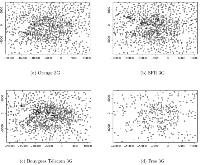
In this chapter, we show that the base stations distribution for an operator and for a technology can be fitted with a -Ginibre point process distribution in several parts of France and that the distribution of all base stations of all operators can be fitted with a Poisson point process. This phenomenon is justified by the theorem stating that the superposition of different -Ginibre point processes converges in distribution to a Poisson point process [44]. Finally we draw conclusions on the coverage-capacity trade-off made by different operators. Qualitative results are derived from the model fitting.

Other existing works on antenna deployment models mainly consider the computation of the SINR and coverage probability for a wide set of point processes. We are instead interested in validating the -Ginibre point process model and the Poisson point process superposition model with real data on a dense urban area. Such a case study is made possible because the French frequency regulator (ANFR) provides location in an open access database [4].

In the first part of this chapter, we give the method to fit the -Ginibre point process model. We consider three scenarios: an urban dense area, a suburban area and a rural area. A qualitative interpretation of the deployment strategies is then provided. In the last part of this chapter, we explore the superposition of -Ginibre point process realizations, and shows that the overall realization converges to the realization of a Poisson point process.

3.2 Point processes and real deployment

3.2.1 Fitting method

The very first step before performing fitting on a real network, is to consider a region in the plane where the density of the points formed by the antennas is globally spatially homoge-neous. This is a reasonable choice since that local homogeneity of the density of antennas is closely linked to the underlying geographical and sociological area. For instance, a densely and homogeneously distributed configuration of antennas might only be found in a densely populated urban area, with high traffic needs. The second step is to derive the intensity of the point process, which is done by counting the antennas in the window considered. The third step is determining the value of the parameter , which proves to be more difficult. Since the law of the number of points is not accessible, it is not possible to deduce factor from the number of points in a subset of compacts. Model fitting is realized using the statistic functions J, since for a -Ginibre, this function is a tractable analytical expression of the coefficient . This summary statistic can be applied because we assume the stationarity of the properties of the realization observed.

We recall that for the -Ginibre, the J function is given in 2 by 8r 2 R⇤+, J (r) =

⇣

(40)

Finding the parameter becomes then a matter of curve fitting. Given a sample of the locations of the base stations, we first consider a window embracing 60% of the surface of the convex hull formed by the sample. The J function estimate is derived for the points inside the window thanks to the function Jest of the R package spatstat [7]. Then the minimum mean square error method is used to fit the theoretical J function onto the estimated J function. Once fitting is performed, the parameter is derived.

3.2.2 Dataset

Real exact data about the locations of every radio emitter in France is available to anyone in an open access database, thanks to the French frequency regulator (ANFR). Operators are obliged by the law to provide accurate information about the location of any of their base stations, which ensures the quality and the accuracy of the data. This database contains the GPS coordinates of each cell, associated with its operator, the technology implemented (2G, 3G, 4G) and the part of the spectrum on which it operates. The -Ginibre point process model is fitted for each scenario, for diﬀerent technologies and bands.

3.2.3 A detailed analysis on Paris networks

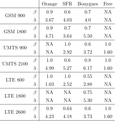
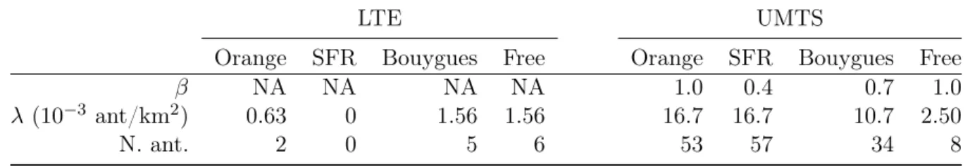
We focus on Paris networks and detail results for each technology and each band. Results in Table 4.1.

Table 3.1: Numerical values of and (base station per km2_{) per technology and operator}

Orange SFR Bouygues Free

GSM 900 0.9 0.6 0.7 NA 3.67 4.03 4.0 NA GSM 1800 0.9 0.7 0.7 NA 4.71 3.64 5.50 NA UMTS 900 NA 1.0 0.6 1.0 NA 2.92 3.72 1.60 UMTS 2100 1.0 0.6 0.8 1.0 4.99 5.27 6.17 1.60 LTE 800 1.0 1.0 0.55 NA 1.03 2.52 2.88 NA LTE 1800 NA NA 0.75 NA NA NA 5.30 NA LTE 2600 0.9 0.64 0.6 1.0 4.23 4.18 3.73 1.60

Among the four operators, Free is the one without a 2G network, since it is a new comer in the market and has only deployed its own 3G and 4G antennas. Furthermore, most operators