Approximating Submodular Functions Everywhere
The MIT Faculty has made this article openly available.
Please share
how this access benefits you. Your story matters.
Citation
Goemans, Michel X. et al. "Approximating Submodular Functions
Everywhere." ACM-SIAM Symposium on Discrete Algorithms, Jan.
4-6, 2009, New York, NY. © 2009 Society for Industrial and Applied
Mathematics.
As Published
http://www.siam.org/proceedings/soda/2009/soda09.php
Publisher
Society for Industrial and Applied Mathematics
Version
Final published version
Citable link
http://hdl.handle.net/1721.1/60671
Terms of Use
Article is made available in accordance with the publisher's
policy and may be subject to US copyright law. Please refer to the
publisher's site for terms of use.
Approximating Submodular Functions Everywhere
Michel X. Goemans
∗Nicholas J. A. Harvey
†Satoru Iwata
‡Vahab Mirrokni
§ AbstractSubmodular functions are a key concept in combina-torial optimization. Algorithms that involve submod-ular functions usually assume that they are given by a (value) oracle. Many interesting problems involving submodular functions can be solved using only polyno-mially many queries to the oracle, e.g., exact minimiza-tion or approximate maximizaminimiza-tion.
In this paper, we consider the problem of approxi-mating a non-negative, monotone, submodular function
f on a ground set of size n everywhere, after only poly(n)
oracle queries. Our main result is a deterministic algo-rithm that makes poly(n) oracle queries and derives a function ˆf such that, for every set S, ˆf (S)
approxi-mates f (S) within a factor α(n), where α(n) = √n + 1
for rank functions of matroids and α(n) = O(√n log n)
for general monotone submodular functions. Our result is based on approximately finding a maximum volume inscribed ellipsoid in a symmetrized polymatroid, and the analysis involves various properties of submodular functions and polymatroids.
Our algorithm is tight up to logarithmic factors. Indeed, we show that no algorithm can achieve a factor better than Ω(√n/ log n), even for rank functions of a
matroid.
1 Introduction Let f : 2[n]→ R
+be a function where [n] = {1, 2, · · · , n}.
The function f is called submodular if
f (S) + f (T ) ≥ f (S ∪ T ) + f (S ∩ T ),
for all S, T ⊆ [n]. Additionally, f is called monotone if f (Y ) ≤ f (Z) whenever Y ⊆ Z. An equivalent definition of submodularity is the property of decreasing
marginal values: For any Y ⊆ Z ⊆ [n] and x ∈ [n] \ Z, f (Z ∪ {x}) − f (Z) ≤ f (Y ∪ {x}) − f (Y ). This can
be deduced from the first definition by substituting
∗MIT Department of Mathematics. [email protected].
Supported by NSF contracts CCF-0515221 and CCF-0829878 and by ONR grant N00014-05-1-0148.
†Microsoft Research New England Lab, Cambridge, MA.
‡RIMS, Kyoto University, Kyoto 606-8502, Japan.
[email protected]. Supported by the Kayamori Foundation of Information Science Advancement.
§Google Research, New York, NY. [email protected].
S = Y ∪ {x} and T = Z; the reverse implication also
holds [28, §44.1]. We assume a value oracle access to the submodular function; i.e., for a given set S, an algorithm can query an oracle to find its value f (S).
Background. Submodular functions are a key con-cept in operations research and combinatorial optimiza-tion, see for example the books [10, 28, 26]; the term ‘submodular’ has over 500 occurrences in Schrijver’s 3-volume book on combinatorial optimization [28]. Sub-modular functions are often considered as a discrete analogue to convex functions; see [23]. Many combina-torial optimization problems can be formulated in terms of submodular functions.
Both minimizing and maximizing submodular func-tions, possibly under some extra constraints, have been considered extensively in the literature. Minimizing submodular functions can be performed efficiently with polynomially many oracle calls, either by the ellip-soid algorithm (see [12]) or through combinatorial al-gorithms that have been obtained in the last decade [29, 14, 15]. Unlike submodular function minimization, the problem of maximizing submodular functions is an NP-hard problem since it generalizes many NP-hard problems such as the maximum cut problem. In many settings, constant-factor approximation algorithms have been developed for this problem. Let us only mention that a 2
5-approximation has been developed for
max-imizing any non-negative, non-monotone submodular function [9], and that a (1 − 1/e)-approximation al-gorithm has been derived for maximizing a monotone submodular function subject to a cardinality constraint [27], or an arbitrary matroid constraint [34]. Approx-imation algorithms for submodular analogues of sev-eral other well-known optimization problems have been studied, e.g., [35, 32].
Submodular functions have been of recent interest due to their applications in combinatorial auctions, par-ticularly the submodular welfare problem [21, 18, 6]. This problem requires partitioning a set of items among a set of players in order to maximize their total utility. In this context, it is natural to assume that the play-ers’ utility functions are submodular, as this captures a realistic notion of diminishing returns. Under this submodularity assumption, efficient approximation al-gorithms have recently been developed for this problem [6, 34].
Contributions. The extensive literature on submod-ular functions motivates us to investigate other fun-damental questions concerning their structure. How much information is contained in a submodular func-tion? How much of that information can be obtained in just a few value oracle queries? Can an auctioneer efficiently estimate a player’s utility function if it is sub-modular? To address these questions, we consider the problem of approximating a submodular function f ev-erywhere while performing only a polynomial number of queries. More precisely, the problem we study is:
Problem 1. Can one make nO(1) queries to
f and construct a function ˆf (not necessarily
submodular) which is an approximation of f , in the sense that ˆf (S) ≤ f (S) ≤ g(n) · ˆf (S)
for all S ⊆ [n]. For what functions g : N → R is this possible?
For some submodular functions this problem can be solved exactly (i.e., with g(n) = 1). As an example, for graph cut functions, it is easy to see that one can completely reconstruct the graph in O(n2) queries.
For more general submodular functions, we prove the following results.
• When f is a rank function of a matroid, we can
compute a function ˆf after a polynomial number
of queries giving an approximation factor g(n) =
√
n + 1. Moreover, ˆf is submodular and has a
particularly simple form: f (S) =ˆ pPi∈Sci for
some c ∈ Rn
+.
• When f is a general monotone submodular
func-tion, we can compute a submodular function ˆf after
a polynomial number of queries giving an approxi-mation factor g(n) = O(√n log n).
• On the other hand, we show that any algorithm
per-forming a polynomial number of queries must sat-isfy g(n) = Ω(√n/ log n), even if f is the rank
func-tion of a matroid. If f is not necessarily monotone, we obtain the lower bound g(n) = Ω(pn/ log n).
Related work. The lower bound mentioned above was previously described in an unpublished manuscript by M. Goemans, N. Harvey, R. Kleinberg and V. Mirrokni. This manuscript also gave a non-adaptive algorithm that solves Problem 1 when f is monotone with g(n) = n/(c log n) for any constant c; furthermore, this is optimal (amongst non-adaptive algorithms).
A subsequent paper of Svitkina and Fleischer [32] considers several new optimization problems on sub-modular functions, as well as Problem 1. They give a randomized algorithm for Problem 1 that applies to a restricted class of submodular functions. Specifically, if there exists R ⊆ [n] such that, for every S ⊆ [n], the
value f (S) depends only on |S∩R| and |S∩ ¯R|, then they
can approximate f everywhere with g(n) = 2√n.
Addi-tionally, Svitkina and Fleischer adjusted the parameters of our lower bound construction, yielding an improved Ω(pn/ log n) lower bound for Problem 1. They also
show that this construction yields nearly-optimal lower bounds for several other problems that they consider.
Not only is our lower bound applicable to other sub-modular problems, but our algorithm is too. For exam-ple, it gives a deterministic O(√n log n)-approximation
algorithm for the non-uniform submodular load balanc-ing problem considered by Svitkina and Fleischer [32], by reducing it to load balancing on unrelated machines. This nearly matches the accuracy of their randomized
O(√n log n)-approximation algorithm. As another
ex-ample, we can reduce the submodular max-min fairness problem [11, 19] to the Santa Claus max-min fair alloca-tion problem [2]. This yields an O(n12m14log n log
3 2
m)-approximation algorithm for the former problem where
m is the number of buyers and n is the number of
items. The existing algorithms for this problem ob-tain a (n − m + approximation [11] and a (2m − 1)-approximation [19]. These applications are discussed in Section 7.
Techniques. Our approximation results are based on ellipsoidal approximations to a centrally symmetric convex body K. An ellipsoid E constitutes a λ-ellipsoidal approximation of K if E ⊆ K ⊆ λE. John’s theorem [16, p203] says that there always exists a √
n-ellipsoidal approximation. We will elaborate on this fact in the following section.
One may also consider ellipsoidal approximations with an algorithmic view. When the body K is given by a separation oracle, it is known how to construct a p
n(n + 1)-ellipsoidal approximation, using only a
poly-nomial number of separation oracle calls. Details are in Gr¨otschel, Lov´asz and Schrijver [12, p124]. Unfortu-nately, this general result is too weak for our purposes. In our case, the convex body K is a symmetrized version of the polymatroid Pfassociated with the
mono-tone submodular function f , and we can exploit symme-tries of this convex body. We show that a (√n +
1/α)-ellipsoidal approximation is achievable for α ≤ 1, pro-vided one can design a α2-approximation algorithm
for the problem of maximizing a convex, separable, quadratic function over Pf. When f is the rank
func-tion of a matroid, this quadratic maximizafunc-tion problem can be solved easily and exactly in polynomial time (us-ing the greedy algorithm), and this gives our √n +
1-approximation for rank functions of matroids. For gen-eral monotone submodular functions, the problem of maximizing (the square root of) a convex, separable,
quadratic function over a polymatroid Pf is equivalent
to the Euclidean norm maximization problem (finding a vector of largest Euclidean norm) over a scaling of the polymatroid Pf. To tackle this latter problem, we
proceed in two steps. We first show that a classical greedy algorithm provides a (1 − 1/e)-approximation al-gorithm for the maximum Euclidean norm problem over a (unscaled) polymatroid Pg; the analysis relies on the
Nemhauser et al. [27] analysis of the greedy algorithm for maximizing a submodular function over a cardinality constraint. We then show that any scaled polymatroid
Q can be approximated by a polymatroid Pg at a loss
of a factor O(log n) (modulo a reasonable condition on the scaling): 1
O(log n)Pg ⊆ Q ⊆ Pg. This step involves
properties of submodular functions (e.g., Lov´asz exten-sions) and polymatroids. Putting these pieces together, we get a O(√n log n)-approximation for any monotone
submodular function everywhere. 2 Ellipsoidal Approximations
In this section, we state and review facts about ellip-soids, we discuss approximations of convex bodies by inscribed and circumscribed ellipsoids, and we build an algorithmic framework that we need for our approxi-mation result. We focus on centrally symmetric convex bodies; in this case, one can exploit polarity to easily switch between inscribed and circumscribed ellipsoids.
In this paper, all matrices that we discuss are n × n, real and symmetric. If a matrix A is positive definite we write A Â 0, and if A is positive semi-definite we write A < 0. Let A Â 0 and let A1/2 be its (unique)
symmetric, positive definite square root: A = A1/2A1/2.
We define the ellipsoidal norm k·kA in Rn by kxkA =
√
xTAx. Let Bndenote the (closed, Euclidean) unit ball
{x ∈ Rn: kxk ≤ 1}, and let V
ndenote its volume. Given
A Â 0, let E(A) denote the ellipsoid (centered at the
origin)
E(A) = { x ∈ Rn : xTAx ≤ 1 } = { x : kxkA ≤ 1 }.
It is the image of the unit ball by a linear map: E(A) =
A−1/2(B
n). The volume of E(A) is Vn/ det(A1/2).
Given c ∈ Rn, we have that
max{ cTx : x ∈ E(A) } = √cTA−1c = kck A−1.
Minimum volume circumscribed ellipsoid. Let
K be a centrally symmetric (x ∈ K iff −x ∈ K) convex
body (compact convex set with non-empty interior) in Rn. The minimum volume ellipsoid circumscribing K
(i.e. containing K) is often referred to as the L¨owner ellipsoid and can be formulated as a semi-infinite pro-gram:
(2.1) min{− log det(A) : kxk2A ≤ 1 ∀x ∈ K
A Â 0 }
where the variables are the symmetric matrix A. Ob-serve that the constraints are linear in A: kxk2
A =
xTAx ≤ 1. One of the main reasons for taking the log
of the volume of the ellipsoid in the objective function is that the determinant of a matrix is strictly log-concave over positive definite matrices.
Lemma 1. (Fan [8]1) Let A, B Â 0, A 6= B, and 0 < λ < 1. Then
log det¡λA+(1−λ)B¢> λ log det A + (1−λ) log det B.
The program (2.1) has therefore a strictly convex objective function (in A) and an infinite number of linear inequalities (in A), and is thus a “nice” convex program. In particular, we can solve the program efficiently provided we can separate over the constraints
kxk2
A ≤ 1. If the convex body K is polyhedral then
we only need to write the constraints kxk2
A ≤ 1 for
its vertices since the maximization of a convex function
xTAx (in x) over a polyhedral set K is always attained
by a vertex. A case of particular interest is when K is defined as the convex hull of a given set of points [17, 20]; this case relates to optimal design problems in statistics.
The strict log-concavity of the determinant shows that the program (2.1) has a unique optimum solution, since a strict convex combination of any two distinct optimum solutions would give a strictly better solu-tion. This shows that the minimum volume ellipsoid is unique, a result which is attributed to L¨owner, and also follows from John’s proof [16].
Maximum volume inscribed ellipsoid. Using po-larity, we can derive a similar formulation for the maxi-mum volume ellipsoid inscribed in K (contained within
K). For a convex body K, its polar K∗ is defined as
{c ∈ Rn : cTx ≤ 1 for all x ∈ K}. Observe that the
po-lar of Bn is Bn itself, and, more generally, the polar of
E(A) is E(A−1). Furthermore, for two convex bodies K
and L, we have that L ⊆ K iff K∗⊆ L∗. Thus, the
max-imum volume ellipsoid E(A) inscribed in K corresponds to the minimum volume ellipsoid E(A−1)
circumscrib-ing K∗. The maximum volume inscribed ellipsoid is
of-ten called the John ellipsoid, although this attribution is somewhat inaccurate since John [16] actually consid-ers only circumscribed ellipsoids. However, as remarked above, circumscribed and inscribed ellipsoids are inter-changeable notions in the centrally symmetric case, so the inaccuracy is forgivable. The John ellipsoid E(A) can be formulated by the following convex semi-infinite 1Fan does not actually state the strict inequality, although his proof does show that it holds.
program polar to (2.1), which maximizes a concave func-tion over a convex set.
max{ log det(A−1) : kck2
A−1 ≤ 1 ∀c ∈ K∗
A−1 Â 0 }
Again, if K is polyhedral, we only need to write the constraint kck2
A−1 ≤ 1 for c such that cTx ≤ 1 defines
a facet of K.
John’s theorem. John’s theorem, well-known in the theory of Banach spaces, says that K is contained in
√
n·E(A), where E(A) is the maximum volume ellipsoid
inscribed in K; in other words, kxkA≤√n for all x ∈ K.
In terms of Banach spaces, this says that the (Banach-Mazur) distance between any n-dimensional Banach space (whose unit ball is K) and the n-dimensional Hilbert space ln 2 is at most √ n.
E(A)
−z
z
John’s theorem can be proved in sev-eral ways. See, for example, Ball [4] or Matouˇsek [24, §13.4]. We adopt a morealgo-rithmic argument. Suppose there is an element z ∈ K with kzkA >
√
n. Then the following lemma gives an
explicit construction of an ellipsoid of strictly larger volume that is contained in the convex hull of E(A),
z and −z, as illustrated in the figure. The resulting
ellipsoid is larger since kn(l) > 1 for l > n. This proves
John’s theorem.
Lemma 2. For A Â 0 and z ∈ Rn with l = kzk2
A ≥ n, let L(A, z) = n l l − 1 n − 1A + n l2 µ 1 − l − 1 n − 1 ¶ AzzTA.
Then L(A, z) is positive definite, the ellipsoid E(L(A, z)) is contained in conv{E(A), {z, −z}},
and its volume vol(E(L(A, z)) equals kn(l) · vol(E(A))
where kn(l) = sµ l n ¶nµ n − 1 l − 1 ¶n−1 .
In this extended abstract, most proofs are deferred to the full version. Actually, the lemma also follows from existing results by considering the polar statement, which says there exists an ellipsoid E(B−1) containing
(2.2) E(A−1) ∩ ©x : −1 ≤ zTx ≤ 1ª
such that vol(E(B−1)) < vol(E(A−1)), assuming
kzkA > √n. See, for example, Gr¨otschel, Lov´asz
and Schrijver [12, p72], Bland, Goldfarb and Todd [5, p1056], and Todd [33]. In fact, Todd derives
an expression for the minimum volume ellipsoid con-taining (2.2), which is precisely B = L(A, z). This shows that E(L(A, z)) is indeed the John ellipsoid for conv{E(A), {z, −z}}.
3 Algorithm for Axis-Aligned Convex Bodies In this section, we consider the question of constructing ellipsoidal approximations efficiently, we show how to exploit symmetries of the convex body, and we relate ellipsoidal approximations to the problem of approxi-mating a submodular function everywhere.
We say that E(A) is a λ-ellipsoidal approximation to K if E(A) ⊆ K and K ⊆ λE(A). The John ellipsoid is therefore a√n-ellipsoidal approximation to a convex
body K, and so is 1/√n times the L¨owner ellipsoid.
These are existential results. Algorithmically, the sit-uation very much depends on how the convex body is given. If it is a polyhedral set given explicitly as the intersection of halfspaces then the convex program for the John’s ellipsoid given above has one constraint for each given inequality and can be solved approximately, to within any desired accuracy. This gives an alter-nate way to derive the result of Gr¨otschel, Lov´asz and Schrijver giving in polynomial-time a√n + 1-ellipsoidal
approximation to a symmetric convex body K given ex-plicitly by a system of linear inequalities. However, if K is given by a separation oracle and comes with the as-sumption of being well-bounded2then the best (known)
algorithmic result is a polynomial-time algorithm giving only apn(n + 1)-ellipsoidal approximation (Gr¨otschel,
Lov´asz, Schrijver [12], Theorem 4.6.3), and this will be too weak for our purpose. In fact, as was pointed out to us by Jos´e Soto, no algorithm, even randomized, can produce an approximation better than ˜O(n) for general
centrally symmetric convex bodies.
The proof given above of John’s theorem can be made algorithmic if we have an α-approximation algo-rithm (α ≤ 1) for maximizing kxkA over x ∈ K and
we are willing to settle for a √n + 1/α-ellipsoidal
ap-proximation. In fact, we only need an α-approximate
decision procedure which, given A Â 0 with E(A) ⊆ K,
either returns an x ∈ K with kxkA >
√
n + 1 or
guar-antees that every x ∈ K satisfies kxkA ≤
√
n + 1/α.
Assume we are given an ellipsoid E0 ⊆ K such that K ⊆ pE0(p is for example R/r in the definition of
well-boundedness, and for our application, we will be able to use p = n). Iteratively, we find larger and larger (multiplicatively in volume) ellipsoids guaranteed to be within K. Given an ellipsoid Ej= E(Aj) at iteration j,
2As part of the input of this centrally symmetric convex body, we get R ≥ r > 0 such that B(0, r) ⊆ K ⊆ B(0, R), and the running time can thus involve log(R/r) polynomially.
suppose we run our α-approximate decision procedure for maximizing kxkAover K. Either (i) it returns a
vec-tor z ∈ K with kzkAj > √ n + 1 or (ii) it guarantees that no x ∈ K satisfies kxkAj > √ n + 1/α. In case of
(ii), we have a√n + 1/α-ellipsoidal approximation. In
case of (i), we can use Lemma 2 to find a larger ellipsoid
Ej+1 = E(Aj+1) also contained within K, and we can
iterate. Our choice of the threshold√n + 1 for the norm
guarantees that vol(Ej+1)/vol(Ej) ≥ 1+4n12−O(1/n3),
as stated in the lemma below. This increase in vol-ume (and the fact that K ⊆ pE0) guarantees that
the number of iterations of this algorithm is at most
O(n2log(pn)) = O(n3log p). One can get a smaller
num-ber of iterations with a higher threshold for the norm, see the Lemma below.
Lemma 3. For the function kn(l) given in Lemma 2,
we have
• kn(n + 1) = 1 +4n12 − O(1/n3), • kn(2n) =
√
2e−1/4− o(1) > 1.
Ellipsoidal approximations for symmetrized polymatroids. Before we proceed, we describe the relationship between the problem of approximating a submodular function everywhere and these ellipsoidal approximations of centrally symmetric convex bodies.
For a monotone, submodular function f : 2[n] → R
with f (∅) = 0, its polymatroid Pf ⊆ Rn is defined by:
P (f ) =
(
x(S) ≤ f (S), ∀S ⊆ [n] x ≥ 0
)
where x(S) =Pi∈Sxi. To make it centrally symmetric,
let S(Q) = { x ∈ Rn : |x| ∈ Q }, where |x| denotes
component-wise absolute value. It is easy to see that, if
f ({i}) > 0 for all i then S(Pf) is a centrally symmetric
convex body. (If there exists an index i with f ({i}) = 0, we can simply get rid of it as monotonicity and submodularity imply that f (S) = f (S − i) for all S with i ∈ S.) Suppose now that E(A) is a λ-ellipsoidal approximation to S(Pf). This implies that, for any
c ∈ Rn,
kckA−1 = max{cTx : x ∈ E(A)} ≤ max{cTx : x ∈ S(P
f)}
≤ λ max{cTx : x ∈ E(A)} = λkckA−1.
In particular, taking c = 1S (the indicator vector for S)
for any S ⊆ [n], we get that
k1SkA−1 ≤ f (S) ≤ λk1SkA−1,
where we have used the fact that max{1T
Sx : x ∈ Pf} =
f (S). Thus the function ˆf defined by ˆf (S) = k1SkA−1
provides a λ-approximation to f (S) everywhere. In summary, a λ-ellipsoidal approximation to S(Pf) gives
a λ-approximation to f (·) everywhere.
Symmetry invariance. However, to be able to get a good ellipsoidal approximation, we need to exploit the symmetries of S(Pf). Observe that if a centrally
symmetric convex body K is invariant under a linear transformation T (i.e. T (K) = K) then, by uniqueness, the maximum volume inscribed ellipsoid E should also be invariant under T . More generally, define the automorphism group of K by Aut(K) = {T (x) = Cx :
T (K) = K}. Then the maximum volume ellipsoid E
inscribed in K satisfies T (E) = E for all T ∈ Aut(K), see for example [13]. In our case, Aut(S(Pf)) contains
all transformations T of the form T (x) = Cx where C is a diagonal ±1 matrix. We call such convex bodies axis
aligned. This means that the maximum volume ellipsoid E(A) inscribed in S(Pf) is also axis aligned, implying
that A is a diagonal matrix.
Algorithm for axis-aligned convex bodies. Un-fortunately, the algorithmic version of John’s theorem presented above does not maintain axis-aligned ellip-soids. Indeed, for a diagonal matrix A, Lemma 2 does not produce an axis-aligned ellipsoid E(L(A, z)). However, we can use the following proposition to map E(L(A, z)) to an ellipsoid of no smaller volume (which shows that the maximum volume ellipsoid is axis aligned). We need some notation. For a vector a ∈ Rn,
let Diag(a) be the diagonal matrix with main diagonal
a; for a matrix A ∈ Rn×n, let diag(A) ∈ Rnbe its main
diagonal.
Proposition 3.1. Let K be an axis-aligned convex
body, and let E(A) be an ellipsoid inscribed in K. Then the ellipsoid E(B) defined by the diagonal matrix B = (Diag(diag(A−1)))−1 satisfies (i) E(B) ⊆ K and
(ii) vol(E(B)) ≥ vol(E(A)).
(ii) is a restatement of Hadamard’s inequality (ap-plied to A−1) which says that for a positive definite
ma-trix C, det(C) ≤ Qni=1cii. To prove (i), one can show
that E(B) ⊆ conv{T (E(A)) : T ∈ Aut(K)}.
Proposition 3.1 shows that, for an axis-aligned convex body such as S(Pf), we can maintain throughout
the algorithm axis-aligned ellipsoids. This has two important consequences. First, this means that we only need an α-approximate decision procedure for the case when A is diagonal. To emphasize this, we rename
A by D. Recall that such a procedure, when given a D Â 0 with E(D) ⊆ S(Pf), either outputs a vector
x ∈ S(Pf) with kxkD >
√
n + 1 or guarantees that kxkD ≤
√
n + 1/α for all x ∈ S(Pf). In section 4, we
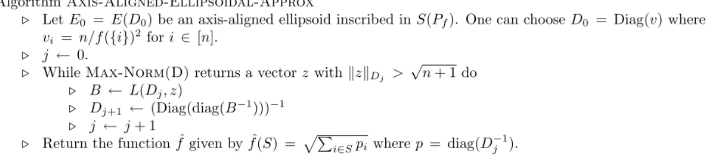
Algorithm Axis-Aligned-Ellipsoidal-Approx
. Let E0 = E(D0) be an axis-aligned ellipsoid inscribed in S(Pf). One can choose D0 = Diag(v) where vi = n/f ({i})2 for i ∈ [n].
. j ← 0.
. While Max-Norm(D) returns a vector z with kzkDj > √
n + 1 do . B ← L(Dj, z)
. Dj+1 ← (Diag(diag(B−1)))−1
. j ← j + 1
. Return the function ˆf given by ˆf (S) = pPi∈Spi where p = diag(D−1j ).
Figure 1: The algorithm for constructing a function ˆf which is a√n + 1/α-approximation to f . x ∈ S(Pf)} can be solved exactly (thus α = 1) and
efficiently (in polynomial time and with polynomially many oracle calls), while in Section 5, we describe an efficient 1/O(log n)-decision procedure for general monotone submodular functions. Secondly, the function
ˆ
f we construct based on an ellipsoidal approximation
takes a particularly simple form when the ellipsoid
E(D) is given by a diagonal matrix D. In this case,
ˆ f (S) = k1SkD−1 reduces to: ˆ f (S) = sX i∈S pi,
where pi = 1/Dii for i ∈ [n]. Observe that this
approximation ˆf is actually submodular (while this was
not necessarily the case for non axis-aligned ellipsoids). Summarizing, Figure 1 gives our algorithm for constructing a √n + 1/α-ellipsoidal approximation of S(Pf) and thus a
√
n + 1/α-approximation to f
ev-erywhere, given an α-approximate decision procedure Max-Norm(D) for maximizing kxkD over S(Pf) (or
equivalently over Pf, by symmetry) for a positive
defi-nite diagonal matrix D (i.e. dii > 0).
One can easily check that the ellipsoid E0= E(D0)
given in the algorithm is an n-ellipsoidal approximation: it satisfies E0 ⊆ S(Pf) and S(Pf) ⊆ nE0.
Theorem 4. If Max-Norm(D) is an α-approximate
decision procedure for max{kxkD : x ∈ Pf} then
Axis-Aligned-Ellipsoidal-Approx outputs a √n + 1/α-approximation to f everywhere after at most O(n3log n) iterations.
4 Matroid Rank Functions
Let M = ([n], I) be a matroid and I its family of independent sets. Let f (·) be its rank function: f (S) = max{|U | : U ⊆ S, U ∈ I} for S ⊆ [n]. f is monotone and submodular and the corresponding polymatroid Pf
is precisely the convex hull of characteristic vectors of independent sets (Edmonds [7]).
For a matroid rank function f , the problem max{kxkD : x ∈ Pf} can be solved exactly in
polynomial-time and with a polynomial number of or-acle calls, when D is a positive definite, diagonal ma-trix. Indeed, maximizing kxkD is equivalent to
max-imizing its square: max©Pidix2i : x ∈ Pf
ª
, where d = diag(D). This is the maximization of a convex
function over a polyhedral set, and therefore the maxi-mum is attained at one of the vertices. But any ver-tex x of Pf is a 0 − 1 vector [7] and thus satisfies
x2
i = xi. The problem is thus equivalent to maximizing
the linear functionPidixi over Pf which can be solved
in polynomial-time by the greedy algorithm for find-ing a maximum weight independent set in a matroid. Therefore, Axis-Aligned-Ellipsoidal-Approx gives a √n + 1-approximation everywhere for rank functions
of matroids.
We should emphasize that the simple approach of linearizing x2
i by xi would have failed if our ellipsoids
were not axis aligned, i.e., if D were not diagonal. In fact, the quadratic spanning tree problem, defined as max{kxkD : x ∈ Pf} where Pf is a graphic matroid
polytope and D is a symmetric, non-diagonal matrix, is NP-hard as it includes the Hamiltonian path problem as a special case [3]. We remark that NP-hardness holds even if D is positive definite.
5 General Monotone Submodular Functions In this section, we present a 1/O(log n)-approximate decision procedure for max{kxkD: x ∈ Pf} for a general
monotone submodular function f . Taking squares, we rewrite the problem as:
(5.3) max ( n X i=1 c2 ix2i : x ∈ Pf ) ,
where we let c = diag(D1/2). Assuming that the
ellipsoid E(D) is inscribed in S(Pf), we will either find
an x ∈ Pf for which
Pn
i=1c2ix2i > n + 1 or guarantee
where α = 1/O(log n).
We first consider the case in which all ci = 1, and
derive a (1 − 1/e)2-approximation algorithm for (5.3).
Consider the following greedy algorithm. Let T0 = ∅,
and for every k = 1, · · · , n, let
Tk = arg max S=Tk−1∪{j}, j /∈Tk−1
f (S),
that is, we repeatedly add the element which gives the largest increase in the submodular function value. Let ˆ
x ∈ Pf be the vector defined by ˆx(Tk) = f (Tk) for
1 ≤ k ≤ n; the fact that ˆx is in Pf is a fundamental
property of polymatroids. We claim that ˆx provides a
(1 − 1/e)2-approximation for (5.3) when all c
i’s are 1.
Lemma 5. For the solution ˆx constructed above, we have n X i=1 ˆ x2 i ≥ µ 1 − 1 e ¶2 max ( n X i=1 x2 i : x ∈ Pf ) .
Proof. Nemhauser, Wolsey and Fisher [27] show that, for every k ∈ [n], we have
f (Tk) ≥ µ 1 −1 e ¶ max S:|S|=kf (S).
Let h(k) = f (Tk) for k ∈ [n]; because of our greedy choice
and submodularity of f , h(·) is concave. Define the monotone submodular function ` by `(S) = e
e−1h(|S|).
The fact that ` is submodular comes from the concavity of h. Observe that, for every S, f (S) ≤ `(S), and therefore, Pf ⊆ P` and max ( n X i=1 x2 i : x ∈ Pf ) ≤ max ( n X i=1 x2 i : x ∈ P` ) .
By convexity of the objective function, the maximum over P` is attained at a vertex. But all vertices of
P` are permutations of the coordinates of e−1e x (or areˆ
dominated by such vertices), and thus max ( n X i=1 x2 i : x ∈ Pf ) ≤ µ e e − 1 ¶2ÃXn i=1 ˆ x2 i ! . ¤ We now deal with the case when the ci’s are
arbitrary. First our guarantee that the ellipsoid E(D) is within S(Pf) means that f ({i})ei(where eiis the ith
unit vector) is not in the interior of E(D), i.e. we must have cif ({i}) ≥ 1 for all i ∈ [n]. We can also assume
that cif ({i}) ≤
√
n + 1. If not, x = f ({i})eiconstitutes
a vector in Pfwith
P
jc2jx2j> n+1. Thus, for all i ∈ [n],
we can assume that 1 ≤ cif ({i}) ≤
√ n + 1.
To reduce to the case with ci = 1 for all i, consider
the linear transformation T : Rn → Rn : x → y =
(c1x1, · · · , cnxn). The problem max{
P
ic2ix2i : x ∈ Pf}
is equivalent to max{Piy2
i : y ∈ T (Pf)}. Unfortunately,
T (Pf) is not a polymatroid, but it is contained in the
polymatroid Pg defined by:
g(S) = max ( X i∈S yi : y ∈ T (Pf) ) = max ( X i∈S cixi : x ∈ Pf ) .
The fact that g is submodular can be derived either from first principles (exploiting the correctness of the greedy algorithm) or as follows. The Lov´asz extension
ˆ
f of f is defined as f : Rn → R : w → max{wTx :
x ∈ Pf} (see Lov´asz [23] or [10]). It is L-convex, see
Murota [25, Prop. 7.25], meaning that, for w1, w2∈ Rn,
ˆ
f (w1) + ˆf (w2) ≥ ˆf (w1∨ w2) + ˆf (w1∧ w2), where ∨
(resp. ∧) denotes component-wise max (resp. min). The submodularity of g now follows from the L-convexity of
ˆ
f by taking vectors w obtained from c by zeroing out
some coordinates.
We can approximately (within a factor (1 − 1/e)2)
compute max{Piy2
i : y ∈ Pg}, or equivalently
approx-imate max{Pic2
ix2i : x ∈ T−1(Pg)}. The question is
how much “bigger” is T−1(P
g) compared to Pf? To
an-swer this question, we perform another polymatroidal approximation, this time of T−1(P
g) and define the
sub-modular function h by:
h(S) = max ( X i∈S xi : x ∈ T−1(Pg) ) = max ( X i∈S 1 ciyi : y ∈ Pg ) .
Again, h(·) is submodular and we can easily obtain a closed form expression for it, see Lemma 8. We have thus sandwiched T−1(P
g) between Pf and Ph:
Pf ⊆ T−1(Pg) ⊆ Ph. To show that all these polytopes
are close to each other, we show the following theorem whose proof is deferred to the full version:
Theorem 6. Suppose that for all i ∈ [n], we have 1 ≤ cif ({i}) ≤
√
n + 1. Then, for all S ⊆ [n], h(S) ≤
¡ 2 + 3
2ln(n)
¢
f (S).
Our algorithm is now the following. Using the (1 − 1/e)2-approximation algorithm applied to P
g, we find a vector ˆx ∈ T−1(P g) such that X i c2ixˆ2i ≥ µ 1 −1 e ¶2 max ( X i c2ix2i : x ∈ T−1(Pg) ) .
Now, by Theorem 6, we know that ˜x = ˆx/O(log n) is in Pf. Therefore, we have that
X i c2 ix˜2i = 1 O(log2(n)) X i c2 ixˆ2i ≥ 1 O(log2(n))max ©P ic2ix2i : x ∈ T−1(Pg) ª ≥ 1 O(log2(n))max ©P ic2ix2i : x ∈ Pf ª ,
giving us the required approximation guarantee. The lemmas below give a closed form expression for g(·) and h(·); their proofs are used in the proof of Theorem 6. They follow from the fact that the greedy algorithm can be used to maximize a linear function over a polymatroid. Both lemmas apply to any set S after renumbering its indices. For any i and j, we define [i, j] = {k ∈ N : i ≤ k ≤ j} and f (i, j) = f ([i, j]). Observe that f (i, j) = 0 for i > j.
Lemma 7. For S = [k] with c1 ≤ c2 ≤ · · · ≤ ck, we
have g(S) = Pki=1ci[f (i, k) − f (i + 1, k)] .
Lemma 8. For S = [k] with c1 ≤ · · · ≤ ck, we have:
h(S) = X i,j : 1≤i≤j≤k ci cj · ³ f (i, j) − f (i + 1, j) −f (i, j − 1) + f (i + 1, j − 1)´ = X l,m : 1≤l≤m≤k (cl− cl−1) µ 1 cm− 1 cm+1 ¶ f (l, m). 6 Lower Bound
In this section, we show that approximating a submod-ular function everywhere requires an approximation ra-tio of Ω¡√n/ log n¢, even when restricting f to be a matroid rank function (and hence monotone). For non-monotone submodular functions, we show that the ap-proximation ratio must be Ω¡pn/ log n¢.
The argument has two steps:
• Step 1. Construct a family of submodular
func-tions parameterized by natural numbers α > β and a set R ⊆ [n] which is unknown to the algorithm.
• Step 2. Use discrepancy arguments to determine
whether a sequence of queries can determine R. This analysis leads to a choice of α and β.
Step 1. Let U be the uniform rank-α matroid on [n]; its rank function is
rU(S) = min {|S|, α} .
Now let R ⊆ [n] be arbitrary such that |R| = α. We define a matroid MR by letting its independent sets be
IMR = { I ⊆ [n] : |I| ≤ α and |I ∩ R| ≤ β } .
This matroid can be viewed as a partition matroid, truncated to rank α. One can check that its rank function is
rMR(S) = min
©
|S|, β + |S ∩ ¯R|, αª.
Now we consider when rU(S) 6= rMR(S). By the
equations above, it is clear that this holds iff (6.4) β + |S ∩ ¯R| < min {|S|, α} .
Case 1: |S| ≤ α. Eq. (6.4) holds iff β + |S ∩ ¯R| < |S|,
which holds iff β < |S ∩ R|. That inequality together with |S| ≤ α implies that |S ∩ ¯R| < α − β.
Case 2: |S| > α. Eq. (6.4) holds iff β + |S ∩ ¯R| < α.
That inequality implies that |S ∩R| > β +(|S|−α) > β. Our family of monotone functions is
F = { rMR : R ⊆ [n], |R| = α } ∪ {rU} .
Our family of non-monotone functions is
F0 = { rMR+ h : R ⊆ [n], |R| = α } ∪ {rU+ h} ,
where h is the function defined by h(S) = −|S|/2. Step 2 (Non-monotone case). Consider any algo-rithm which is given a function f ∈ F0, performs a
se-quence of queries f (S1), . . . , f (Sk), and must distinguish
whether f = rU+ h or f = rMR+ h (for some R). For
the sake of distinguishing these possibilities, the added function h is clearly irrelevant; it only affects the ap-proximation ratio. By our discussion above, the algo-rithm can distinguish rMR from rU only if one of the
following two cases occurs.
Case 1: ∃i such that |Si| ≤ α and |Si∩ R| > β.
Case 2: ∃i such that |Si| > α and β + |Si∩ ¯R| < α.
As argued above, if either of these cases hold then we have both |Si∩ R| > β and |Si∩ ¯R| < α − β. Thus
(6.5) |Si∩ R| − |Si∩ ¯R| > 2β − α.
Now consider the family of sets A = {S1, . . . , Sk, [n]}. A
standard result [1, Theorem 12.1.1] on the discrepancy of A shows that there exists an R such that
¯ ¯ |Si∩ R| − |Si∩ ¯R| ¯ ¯ ≤ ² ∀i (6.6a) ¯ ¯ |[n] ∩ R| − |[n] ∩ ¯R|¯¯ ≤ ², (6.6b)
where ² = p2n ln(2k). Eq. (6.6b) implies that |R| =
n/2 + ²0, where |²0| ≤ ²/2. By definition, α = |R|. So if
we choose β = n/4 + ² then 2β − α > ². Thus Eq. (6.5) cannot hold, since it would contradict Eq. (6.6a). This shows that the algorithm cannot distinguish f = rMR+h
from f0 = r
The approximation ratio of the algorithm is at most
f0(R)/f (R). We have f0(R) = |R| − |R|/2 = |R|/2
and f (R) = β − |R|/2 ≤ (n/4 + ²) − (n/2 − ²)/2 < 2². This shows that no deterministic algorithm can achieve approximation ratio better than
f0(R) f (R) = |R| 4² ≥ n/2 − ² 4² = Ω( p n/ log k)
Since k = nO(1), this proves the claimed result. If
k = O(n) then the lower bound improves to Ω(√n) via
a result of Spencer [30].
The construction of the set R in [1, Theorem 12.1.1] is probabilistic: choosing R uniformly at random works with high probability, regardless of the algorithm’s queries S1, . . . , Sk. This implies that the lower bound
also applies to randomized algorithms.
Step 2 (Monotone case). In this case, we pick α ≈
√
n and β = Ω(ln k). The argument is similar to the
non-monotone case except that we cannot apply standard discrepancy results since they do not construct R with
|R| = α ≈ √n. Instead, we derive analogous results
using Chernoff bounds. We construct R by picking each element independently with probability 1/√n. With
high probability |R| = Θ(√n). We must now bound
the probability that the algorithm succeeds.
Case 1: Given |Si| ≤ α, what is Pr [ |Si∩ R| > β ]? We
have E [ |R ∩ Si| ] = |Si|/√n = O(1). Chernoff bounds
show that Pr [ |R ∩ Si| > β ] ≤ exp(−β/2) = 1/k2.
Case 2: Given |Si| > α, what is Pr
£
β + |Si∩ ¯R| < α
¤ ? As observed above, this event is equivalent to |Si∩ R| >
β + (|Si| − α) =: ξ. Let µ = E £ |Si∩ ¯R| ¤ = |Si|/ √ n. Note that ξ µ = log n |Si|/ √ n+ √ n · ³ 1 − α |Si| ´ ,
which is Ω(log n) for any value of |Si|. A Chernoff bound
then shows that Pr [ |Si∩ R| > ξ ] < exp(−ξ/2) ≤ 1/k2.
A union bound shows that none of these events oc-cur with high probability, and thus the algorithm fails to distinguish rMR from rU. The approximation
ra-tio of the algorithm is at most f0(R)/f (R) = α/β =
Ω(√n/ log k). This lower bound also applies to
ran-domized algorithms, by the same reasoning as in the non-monotone case. Since k = nO(1), this proves the
desired result. 7 Applications
7.1 Submodular Load Balancing
Let f1, . . . , fm be monotone submodular functions on
the ground set [n]. The non-uniform submodular load balancing problem is
(7.7) min
V1,...,Vm
max
j fj(Vj),
where the minimization is over partitions of [n] into
V1, . . . , Vm.
Suppose we construct the approximations ˆ
f1, . . . , ˆfmsuch that
ˆ
fj(S) ≤ fj(S) ≤ g(n) · ˆfj(S) ∀j ∈ [m], S ⊆ [n].
Furthermore, suppose that each ˆfj is of the form
ˆ
fj(S) =
sX
i∈S
cj,i,
for some non-negative real values cj,i. Consider the
problem of finding a partition V1, . . . , Vmthat minimizes
maxjfˆj(Vj). By squaring, we would like to solve
(7.8) min V1,...,Vm max j X i∈Vj cj,i.
This is precisely the problem of scheduling jobs without preemption on non-identical parallel machines, while minimizing the makespan. In deterministic polyno-mial time, one can compute a 2-approximate solution
X1, . . . , Xm to this problem [22], which also gives an
approximate solution to Eq. (7.7).
Formally, let W1, . . . , Wmbe an optimal solution to
Eq. (7.8), let X1, . . . , Xmbe a solution computed using
the algorithm of [22], and let Y1, . . . , Ymbe an optimal
solution to the original problem in Eq. (7.7). Then we have 1
2· maxjfˆj2(Xj) ≤ maxjfˆj2(Wj), and thus
1
√
2g(n)· maxj fj(Xj) ≤ maxj fj(Yj).
Thus, the Xj’s give a (
√
2 g(n))-approximate solution to Eq. (7.7). Applying the algorithm of Section 5 to con-struct the ˆfj’s, we obtain an O(
√
n log n)-approximation
to the non-uniform submodular load balancing problem. 7.2 Submodular Max-Min Fair Allocation Consider m buyers and a ground set [n] of items. Let
f1, . . . , fm be monotone submodular functions on the
ground set [n], and let fj be the valuation function
of buyer j. The submodular max-min fair allocation problem is
(7.9) max
V1,...,Vm
min
j fj(Vj),
where the maximization is over partitions of [n] into
V1, . . . , Vm. This problem was studied by Golovin [11]
and Khot and Ponnuswami [19]. Those papers re-spectively give algorithms achieving an (n − m + 1)-approximation and a (2m − 1)-1)-approximation. Here we
give a O(n12m14log n log 3
2m)-approximation algorithm
for this problem.
The idea of the algorithm is similar to that of the load balancing problem. We construct the approxima-tions ˆf1, . . . , ˆfm
ˆ
fj(S) ≤ fj(S) ≤ g(n) · ˆfj(S) ∀j ∈ [m], S ⊆ [n],
such that ˆfj is of the form
ˆ
fj(S) =
sX
i∈S
cj,i,
for some non-negative real values cj,i. Consider the
problem of finding a partition V1, . . . , Vm that
maxi-mizes minjfˆj(Vj). By squaring, we would like to solve
max V1,...,Vm min j X i∈Vj cj,i.
This problem is the Santa Claus max-min fair allocation problem, for which Asadpour and Saberi [2] give a
O(√m log3m) approximation algorithm. Using this, together with the algorithm of Section 5 to construct the
ˆ fj’s, we obtain an O(n 1 2m14log n log 3 2m)-approximation
for the submodular max-min fair allocation problem. Acknowledgements
The authors thank Robert Kleinberg for helpful discus-sions at a preliminary stage of this work, Jos´e Soto for discussions on inertial ellipsoids, and Uri Feige for his help with the analysis of Section 6.
References
[1] N. Alon and J. Spencer. “The Probabilistic Method”. Wiley, second edition, 2000.
[2] A. Asadpour and A. Saberi. “An approximation algorithm for max-min fair allocation of indivisible goods”. STOC, 114–121, 2007.
[3] A. Assad and W. Xu. “The Quadratic Minimum Spanning Tree Problem”. Naval Research Logistics, 39, 1992. [4] K. Ball. “An Elementary Introduction to Modern Convex
Geometry”. Flavors of Geometry, MSRI Publications, 1997. [5] R. G. Bland, D. Goldfarb and M. J. Todd. “The Ellipsoid
Method: A Survey”. Operations Research, 29, 1981. [6] S. Dobzinski and M. Schapira. “An improved
approxima-tion algorithm for combinatorial aucapproxima-tions with submodular bidders”. SODA, 1064–1073, 2006.
[7] J. Edmonds, “Matroids and the Greedy Algorithm”,
Math-ematical Programming, 1, 127–136, 1971.
[8] K. Fan, “On a theorem of Weyl concerning the eigenvalues of linear transformations, II”, Proc. Nat. Acad. Sci., 1950. [9] U. Feige, V. Mirrokni and J. Vondr´ak, “Maximizing
non-monotone submodular functions”, FOCS, 461–471, 2007. [10] S. Fujishige, “Submodular Functions and Optimization”,
volume 58 of Annals of Discrete Mathematics. Elsevier, second edition, 2005.
[11] D. Golovin, “Max-Min Fair Allocation of Indivisible Goods”. Technical Report CMU-CS-05-144, 2005.
[12] M. Gr¨otschel, L. Lov´asz, and A. Schrijver, “Geometric Algo-rithms and Combinatorial Optimization”, Springer Verlag, second edition, 1993.
[13] O. G¨uler and F. G¨urtina, “The extremal volume ellipsoids of convex bodies, their symmetry properties, and their determination in some special cases”, arXiv:0709.707v1. [14] S. Iwata, L. Fleischer, and S. Fujishige, “A combinatorial,
strongly polynomial-time algorithm for minimizing submod-ular functions”, Journal of the ACM, 48, 761–777, 2001. [15] S. Iwata and J. Orlin, “A Simple Combinatorial Algorithm
for Submodular Function Minimization”, SODA, 2009. [16] F. John. “Extremum problems with inequalities as
sub-sidiary conditions”, Studies and Essays, presented to R.
Courant on his 60th Birthday, January 8, 1948,
Inter-science, New York, 187–204, 1948.
[17] L. G. Khachiyan. “Rounding of polytopes in the real number model of computation”, Math of OR, 21, 307–320, 1996. [18] S. Khot, R. Lipton, E. Markakis and A. Mehta.
“Inapprox-imability results for combinatorial auctions with submodu-lar utility functions”, WINE, 92–101, 2005.
[19] S. Khot and A. Ponnuswami. “Approximation Algo-rithms for the Max-Min Allocation Problem”.
APPROX-RANDOM, 204–217, 2007.
[20] P. Kumar and E. A. Yıldırım, “Minimum-Volume Enclosing Ellipsoids and Core Sets”, Journal of Optimization Theory
and Applications, 126, 1–21, 2005.
[21] B. Lehmann, D. J. Lehmann and N. Nisan. “Combinatorial auctions with decreasing marginal utilities”, Games and
Economic Behavior, 55, 270–296, 2006.
[22] J. K. Lenstra, D. B. Shmoys and E. Tardos. “Approxima-tion algorithms for scheduling unrelated parallel machines”.
Mathematical Programming, 46, 259–271, 1990.
[23] L. Lov´asz, “Submodular Functions and Convexity”, in A. Bachem et al., eds, Mathematical Programmming: The State of the Art, 235–257, 1983.
[24] J.Matouˇsek, “Lectures on Discrete Geometry”. Springer, 2002.
[25] K. Murota, “Discrete Convex Analysis”, SIAM Monographs on Discrete Mathematics and Applications, SIAM, 2003. [26] H. Narayanan, “Submodular Functions and Electrical
Net-works”, Elsevier, 1997.
[27] G. L. Nemhauser, L. A. Wolsey and M. L. Fisher. “An analysis of approximations for maximizing submodular set functions I”. Mathematical Programming, 14, 1978. [28] A. Schrijver, “Combinatorial Optimization: Polyhedra and
Efficiency”. Springer, 2004.
[29] A. Schrijver, “A combinatorial algorithm minimizing sub-modular functions in strongly polynomial time”, Journal of
Combinatorial Theory, Series B, 80, 346–355, 2000.
[30] J. Spencer, “Six Standard Deviations Suffice”, Trans. Amer.
Math. Soc., 289, 679–706, 1985.
[31] P. Sun and R. M. Freund. “Computation of Minimum Volume Covering Ellipsoids”, Operations Research, 52, 690–706, 2004.
[32] Z. Svitkina and L. Fleischer. “Submodular Approximation: Sampling-Based Algorithms and Lower Bounds”. FOCS, 2008.
[33] M. J. Todd. “On Minimum Volume Ellipsoids Containing Part of a Given Ellipsoid”. Math of OR, 1982.
[34] J. Vondr´ak. “Optimal Approximation for the Submodular Welfare Problem in the Value Oracle Model”. STOC, 2008. [35] L. A. Wolsey. “An Analysis of the Greedy Algorithm for the Submodular Set Covering Problem”. Combinatorica, 2, 385–393, 1982.