Approximating the noise sensitivity of a monotone Boolean function

Approximating the noise sensitivity of a monotone Boolean

function

by

Arsen Vasilyan

B.S., Massachusetts Institute of Technology (2019)

Submitted to the Department of Electrical Engineering and Computer

Science

in partial fulfillment of the requirements for the degree of

Master of Science in Computer Science and Engineering

at the

MASSACHUSETTS INSTITUTE OF TECHNOLOGY

May 2020

c

○ Massachusetts Institute of Technology 2020. All rights reserved.

Author . . . .

Department of Electrical Engineering and Computer Science

May 15, 2020

Certified by . . . .

Ronitt Rubinfeld

Professor of Electrical Engineering and Computer Science

Thesis Supervisor

Accepted by . . . .

Leslie A. Kolodziejski

Professor of Electrical Engineering and Computer Science

Chair, Department Committee on Graduate Students

Approximating the noise sensitivity of a monotone Boolean function

by

Arsen Vasilyan

Submitted to the Department of Electrical Engineering and Computer Science on May 15, 2020, in partial fulfillment of the

requirements for the degree of

Master of Science in Computer Science and Engineering

Abstract

The noise sensitivity of a Boolean function 𝑓 : {0, 1}𝑛 → {0, 1} is one of its fundamental properties. For noise parameter 𝛿, the noise sensitivity is denoted as 𝑁 𝑆𝛿[𝑓 ]. This quantity

is defined as follows: First, pick 𝑥 = (𝑥1, . . . , 𝑥𝑛) uniformly at random from {0, 1}𝑛, then

pick 𝑧 by flipping each 𝑥𝑖 independently with probability 𝛿. 𝑁 𝑆𝛿[𝑓 ] is defined to equal

Pr[𝑓 (𝑥) ̸= 𝑓 (𝑧)]. Much of the existing literature on noise sensitivity explores the follow-ing two directions: (1) Showfollow-ing that functions with low noise-sensitivity are structured in certain ways. (2) Mathematically showing that certain classes of functions have low noise sensitivity. Combined, these two research directions show that certain classes of functions have low noise sensitivity and therefore have useful structure.

The fundamental importance of noise sensitivity, together with this wealth of structural results, motivates the algorithmic question of approximating 𝑁 𝑆𝛿[𝑓 ] given an oracle access

to the function 𝑓 . We show that the standard sampling approach is essentially optimal for general Boolean functions. Therefore, we focus on estimating the noise sensitivity of monotonefunctions, which form an important subclass of Boolean functions, since many functions of interest are either monotone or can be simply transformed into a monotone function (for example the class of unate functions consists of all the functions that can be made monotone by reorienting some of their coordinates [22]).

Specifically, we study the algorithmic problem of approximating 𝑁 𝑆𝛿[𝑓 ] for

mono-tone 𝑓 , given the promise that 𝑁 𝑆𝛿[𝑓 ] ≥ 1/𝑛𝐶 for constant 𝐶, and for 𝛿 in the range

1/𝑛 ≤ 𝛿 ≤ 1/2. For such 𝑓 and 𝛿, we give a randomized algorithm that has query com-plexity of 𝑂(︁min(1, √ 𝑛𝛿 log1.5_𝑛) 𝑁 𝑆𝛿[𝑓 ] poly (︁ 1 𝜖 )︁)︁

and approximates 𝑁 𝑆𝛿[𝑓 ] to within a

multiplica-tive factor of (1 ± 𝜖). Given the same constraints on 𝑓 and 𝛿, we also prove a lower bound of Ω(︁min(1,

√

𝑛𝛿) 𝑁 𝑆𝛿[𝑓 ]·𝑛𝜉

)︁

on the query complexity of any algorithm that approximates 𝑁 𝑆𝛿[𝑓 ] to

within any constant factor, where 𝜉 can be any positive constant. Thus, our algorithm’s query complexity is close to optimal in terms of its dependence on 𝑛.

We introduce a novel descending-ascending view of noise sensitivity, and use it as a central tool for the analysis of our algorithm. To prove lower bounds on query complexity, we develop a technique that reduces computational questions about query complexity to combinatorial questions about the existence of “thin" functions with certain properties.

The existence of such “thin" functions is proved using the probabilistic method. These techniques also yield new lower bounds on the query complexity of approximating other fundamental properties of Boolean functions: the total influence and the bias.

Thesis Supervisor: Ronitt Rubinfeld

Acknowledgments

I am indebted to Ronitt Rubinfeld for suggesting the problem and supervising this work. I also would like to express my sincere gratitude to my family for their unconditional trust and encouragement.

Contents

1 Introduction 11

1.1 Results . . . 14

1.2 Algorithm overview . . . 16

1.3 Lower bound techniques . . . 21

1.4 Possibilities of improvement? . . . 24

2 Preliminaries 27 2.1 Definitions . . . 27

2.1.1 Fundamental definitions and lemmas pertaining to the hypercube. . 27

2.1.2 Fundamental definitions pertaining to Boolean functions . . . 28

2.1.3 Influence estimation. . . 29

2.1.4 Bounds for 𝜖 and 𝐼[𝑓 ] . . . 30

3 An improved algorithm for small 𝛿 31 3.1 Descending-ascending framework . . . 31

3.1.1 The descending-ascending process. . . 31

3.1.2 Defining bad events . . . 32

3.1.3 Defining 𝑝𝐴, 𝑝𝐵 . . . 33

3.1.4 Bad events can be “ignored” . . . 35

3.2 Main lemmas . . . 35

3.4 Sampling descending and ascending paths going through a given influential

edge. . . 42

3.5 The noise sensitivity estimation algorithm. . . 53

4 Lower bounding the query complexity. 57 4.1 Proof of Lemma 4.0.3 . . . 61 4.2 Proof of Lemma 4.0.4 . . . 64 4.3 Proof of (a) . . . 64 4.4 Proof of b) . . . 65 4.5 Proof of c) . . . 66 4.6 Proof of d) . . . 68 A Appendix A 75 B A query complexity lower bound for general Boolean functions 77 C Proofs of technical lemmas pertaining to the algorithm 81 C.1 Appendix C . . . 81

C.2 Proof of Lemma 2.1.1 . . . 81

C.3 Proof of Lemma 3.1.3 . . . 83

C.4 Proof of Lemma 3.5.3 . . . 84

C.5 Proof of Lemma 3.5.4 . . . 84

D Proofs of technical lemmas pertaining to query complexity lower bounds 87 D.1 Proof of Lemma 4.0.1 . . . 87

List of Figures

1-1 The noise process . . . 17

1-2 Algorithm for sampling an influential edge . . . 19

1-3 Algorithm 𝒲 . . . 20

1-4 Algorithm ℬ . . . 21

1-5 Algorithm for estimating noise sensitivity. . . 22

3-1 The noise process (restated) . . . 32

3-2 Algorithm for sampling an influential edge (restated) . . . 37

3-3 Algorithm 𝒲 (restated) . . . 44

3-4 Algorithm ℬ (restated) . . . 50

Chapter 1

Introduction

Noise sensitivity is a property of any Boolean function 𝑓 : {0, 1}𝑛 _{→ {0, 1} defined as}

follows: First, pick 𝑥 = (𝑥1, . . . , 𝑥𝑛) uniformly at random from {0, 1}𝑛, then pick 𝑧 by

flipping each 𝑥𝑖 independently with probability 𝛿. Here 𝛿, the noise parameter, is a given

positive constant no greater than 1/2 (and at least 1/𝑛 in the interesting cases). With the above distributions on 𝑥 and 𝑧, the noise sensitivity of 𝑓 , denoted as 𝑁 𝑆𝛿[𝑓 ], is defined as

follows:

𝑁 𝑆𝛿[𝑓 ]

def

= Pr[𝑓 (𝑥) ̸= 𝑓 (𝑧)] (1.1)

Noise sensitivity was first explicitly defined by Benjamini, Kalai and Schramm in [3], and has been the focus of multiple papers: e.g. [3, 7, 8, 10, 11, 13, 18, 23]. It has been applied to learning theory [4, 7, 8, 9, 11, 12, 16], property testing [1, 2], hardness of approxima-tion [14, 17], hardness amplificaapproxima-tion [20], theoretical economics and political science[10], combinatorics [3, 13], distributed computing [19] and differential privacy [7]. Multiple properties and applications of noise sensitivity are summarized in [21] and [22]. Much of the existing literature on noise sensitivity explores the following directions: (1) Showing that functions with low noise-sensitivity are structured in certain ways. (2) Mathematically showing that certain classes of functions have low noise sensitivity. Combined, these two research directions show that certain classes of functions have low noise sensitivity and therefore have useful structure.

results, motivates the algorithmic question of approximating 𝑁 𝑆𝛿[𝑓 ] given an oracle access

to the function 𝑓 . It can be shown that standard sampling techniques require 𝑂(︁_{𝑁 𝑆}1

𝛿[𝑓 ]𝜖2

)︁

queries to get a (1 + 𝜖)-multiplicative approximation for 𝑁 𝑆𝛿[𝑓 ]. In Appendix B, we show

that this is optimal for a wide range of parameters of the problem. Specifically, it cannot be improved by more than a constant when 𝜖 is a sufficiently small constant, 𝛿 satisfies 1/𝑛 ≤ 𝛿 ≤ 1/2 and 𝑁 𝑆𝛿[𝑓 ] satisfies Ω

(︁₁

2𝑛

)︁

≤ 𝑁 𝑆𝛿[𝑓 ] ≤ 𝑂(1).

It is often the case that data possesses a known underlying structural property which makes the computational problem significantly easier to solve. A natural first such property to investigate is that of monotonicity, as a number of natural function families are made up of functions that are either monotone or can be simply transformed into a monotone function (for example the class of unate functions consists of all the functions that can be made monotone by reorienting some of their coordinates [22]). Therefore, we focus on estimating the noise sensitivity of monotone functions.

The approximation of the related quantity of total influence (henceforth just influence) of a monotone Boolean function in this model was previously studied by [25, 24]1_.

In-fluence, denoted by 𝐼[𝑓 ], is defined as 𝑛 times the probability that a random edge of the Boolean cube (𝑥, 𝑦) is influential, which means that 𝑓 (𝑥) ̸= 𝑓 (𝑦). (This latter probabil-ity is sometimes referred to as the average sensitivprobabil-ity). It was shown in [25, 24] that one can approximate the influence of a monotone function 𝑓 with only ˜𝑂(︁

√

𝑛 𝐼[𝑓 ]poly(𝜖)

)︁

queries, which for constant 𝜖 beats the standard sampling algorithm by a factor of √𝑛, ignoring

logarithmic factors.

Despite the fact that the noise sensitivity is closely connected to the influence [21, 22], the noise sensitivity of a function can be quite different from its influence. For instance, for the parity function of all 𝑛 bits, the influence is 𝑛, but the noise sensitivity is 1₂(1 − (1 − 2𝛿)𝑛_{) (such disparities also hold for monotone functions, see for example the discussion of}

influence and noise sensitivity of the majority function in [22]). Therefore, approximating the influence by itself does not give one a good approximation to the noise sensitivity.

The techniques in [25, 24] also do not immediately generalize to the case of noise

1_{[24] is the journal version of [25] and contains a different algorithm that yields sharper results. However,}

sensitivity. The result in [25, 24] is based on the observation that given a descending2path on the Boolean cube, at most one edge in it can be influential. Thus, to check if a descending path of any length contains an influential edge, it suffices to check the function values at the endpoints of the path. By sampling random descending paths, [25, 24] show that one can estimate the fraction of influential edges, which is proportional to the influence.

The most natural attempt to relate these path-based techniques with the noise sensitivity is to view it in the context of the following process: first one samples 𝑥 randomly, then one obtains 𝑧 by taking a random walk from 𝑥 by going through all the indices in an arbitrary order and deciding whether to flip each with probability 𝛿. The intermediate values in this process give us a natural path connecting 𝑥 to 𝑧. However, this path is in general not descending, so it can, for example, cross an even number of influential edges, and then the function will have the same value on the two endpoints of this path. This prevents one from immediately applying the techniques from [25, 24].

We overcome this difficulty by introducing our main conceptual contribution: the descending-ascending view of noise sensitivity. In the process above, instead of going through all the indices in an arbitrary order, we first go through the indices 𝑖 for which

𝑥𝑖 = 1 and only then through the ones for which 𝑥𝑖 = 0. This forms a path between 𝑥 and 𝑧 that has first a descending component and then an ascending component. Although this

random walk is more amenable to an analysis using the path-based techniques of [25, 24], there are still non-trivial sampling questions involved in the design and analysis of our algorithm.

An immediate corollary of our result is a query complexity upper bound on estimating the gap between the noise stability of a Boolean function and one. The noise stability of a Boolean function 𝑓 depends on a parameter 𝜌 and is denoted by Stab𝜌[𝑓 ] (for more

infor-mation about noise stability, see [22]). One way Stab𝜌[𝑓 ] can be defined is as the unique

quantity satisfying the functional relation 1₂(1 − Stab1−2𝛿[𝑓 ]) = 𝑁 𝑆𝛿[𝑓 ] for all 𝛿. This

im-plies that by obtaining an approximation for 𝑁 𝑆𝛿[𝑓 ], one also achieves an approximation

for 1 − Stab1−2𝛿[𝑓 ].

2_{A path is descending if each subsequent vertex in it is dominated by all the previous ones in the natural}

1.1

Results

Our main algorithmic result is the following:

Theorem 1 Let 𝛿 be a parameter satisfying:

1

𝑛 ≤ 𝛿 ≤

1 √

𝑛 log1.5𝑛

Suppose,𝑓 : {0, 1}𝑛_{→ {0, 1} is a monotone function and 𝑁 𝑆}

𝛿[𝑓 ] ≥ _𝑛1𝐶 for some constant

𝐶.

Then, there is an algorithm that outputs an approximation to𝑁 𝑆𝛿[𝑓 ] to within a

multi-plicative factor of(1 ± 𝜖), with success probability at least 2/3. In expectation, the algo-rithm makes𝑂(︁

√

𝑛𝛿 log1.5_𝑛

𝑁 𝑆𝛿[𝑓 ]𝜖3

)︁

queries to the function. Additionally, it runs in time polynomial in𝑛.

Note that computing noise-sensitivity using standard sampling3 _{requires 𝑂}(︁ 1

𝑁 𝑆𝛿[𝑓 ]𝜖2

)︁

samples. Therefore, for a constant 𝜖, we have the most dramatic improvement if 𝛿 = _𝑛1, in which case, ignoring constant and logarithmic factors, our algorithm outperforms standard sampling by a factor of√𝑛.

As in [25], our algorithm requires that the noise sensitivity of the input function 𝑓 is larger than a specific threshold 1/𝑛𝐶. Our algorithm is not sensitive to the value of 𝐶 as long as it is a constant, and we think of 1/𝑛𝐶 _{as a rough initial lower bound known in}

advance.

We next give lower bounds for approximating three different parameters of monotone Boolean functions: the bias, the influence and the noise sensitivity. A priori, it is not clear what kind of lower bounds one could hope for. Indeed, determining whether a given func-tion is the all-zeros funcfunc-tion requires Ω(2𝑛) queries in the general function setting, but only 1 query (of the all-ones input), if the function is promised to be monotone. Nevertheless, we show that such a dramatic improvement for approximating these quantities is not possible.

3_{Standard sampling refers to the algorithm that picks 𝑂}(︁ 1

𝑁 𝑆𝛿[𝑓 ]𝜖2

)︁

pairs 𝑥 and 𝑧 as in the definition of noise sensitivity and computes the fraction of pairs for which 𝑓 (𝑥) ̸= 𝑓 (𝑧).

For monotone functions, we are not aware of previous lower bounds on approximating the bias or noise sensitivity. Our lower bound on approximating influence is not comparable to the lower bounds in [25, 24], as we will elaborate shortly.

We now state our lower bound for approximating the noise sensitivity. Here and every-where else, to “reliably distinguish" means to distinguish with probability at least 2/3.

Theorem 2 For all constants 𝐶1and𝐶2satisfying𝐶1−1 > 𝐶2 ≥ 0, for an infinite number

of values of𝑛 the following is true: For all 𝛿 satisfying 1/𝑛 ≤ 𝛿 ≤ 1/2, given a monotone

function𝑓 : {0, 1}𝑛 _{→ {0, 1}, one needs at least Ω}(︁ 𝑛𝐶2

𝑒

√

𝐶1 log 𝑛/2

)︁

queries to reliably distin-guish between the following two cases: (i)𝑓 has noise sensitivity between Ω(1/𝑛𝐶1+1_{) and}

𝑂(1/𝑛𝐶1_{) and (ii) 𝑓 has noise sensitivity larger than Ω(min(1, 𝛿}√_𝑛)/𝑛𝐶2_).

Remark 1 For any positive constant 𝜉, we have that 𝑒 √

𝐶1log 𝑛/2 _{≤ 𝑛}𝜉_.

Remark 2 The range of the parameter 𝛿 can be divided into two regions of interest. In the region 1/𝑛 ≤ 𝛿 ≤ 1/(√𝑛 log 𝑛), the algorithm from Theorem 1 can distinguish the

two cases above with only ˜𝑂(𝑛𝐶2_{) queries. Therefore its query complexity is optimal up}

to a factor of ˜𝑂(𝑒

√

𝐶1log 𝑛/2_{). Similarly, in the region 1/(}√_{𝑛 log 𝑛) ≤ 𝛿 ≤ 1/2, the}

stan-dard sampling algorithm can distinguish the two distributions above with only ˜𝑂(𝑛𝐶2₎

queries. Therefore in this region of interest, standard sampling is optimal up to a factor of ˜

𝑂(𝑒

√

𝐶1log 𝑛/2_).

We define the bias of a Boolean function as 𝐵[𝑓 ] def= Pr[𝑓 (𝑥) = 1], where 𝑥 is chosen uniformly at random from {0, 1}𝑛. It is arguably the most basic property of a Boolean function, so we consider the question of how quickly it can be approximated for monotone functions. To approximate the bias up to a multiplicative factor of 1 ± 𝜖 using standard sampling, one needs 𝑂(1/(𝐵[𝑓 ]𝜖2_{)) queries. We obtain a lower bound for this task similar}

to the previous theorem:

Theorem 3 For all constants 𝐶1and𝐶2satisfying𝐶1−1 > 𝐶2 ≥ 0, for an infinite number

one needs at leastΩ(︁ 𝑛𝐶2 𝑒

√

𝐶1 log 𝑛/2

)︁

queries to reliably distinguish between the following two cases: (i)𝑓 has bias of Θ(1/𝑛𝐶1_{) (ii) 𝑓 has bias larger than Ω(1/𝑛}𝐶2_).

Finally we prove a lower bound for approximating influence:

Theorem 4 For all constants 𝐶1and𝐶2satisfying𝐶1−1 > 𝐶2 ≥ 0, for an infinite number

of values of 𝑛 the following is true: Given a monotone function 𝑓 : {0, 1}𝑛 _{→ {0, 1},}

one needs at leastΩ(︁ 𝑛𝐶2 𝑒

√

𝐶1 log 𝑛/2

)︁

queries to reliably distinguish between the following two cases: (i)𝑓 has influence between Ω(1/𝑛𝐶1_{) and 𝑂(𝑛/𝑛}𝐶1_{) (ii) 𝑓 has influence larger than}

Ω(√𝑛/𝑛𝐶2_).

This gives us a new sense in which the algorithm family in [25, 24] is close to optimal, because for a function 𝑓 with influence Ω(√𝑛/𝑛𝐶2_{) this algorithm makes ˜𝑂(𝑛}𝐶2_{) queries}

to estimate the influence up to any constant factor.

Our lower bound is incomparable to the lower bound in [25], which makes the stronger requirement that 𝐼[𝑓 ] ≥ Ω(1), but gives a bound that is only a polylogarithmic factor smaller than the runtime of the algorithm in [25, 24]. There are many possibilities for algo-rithmic bounds that were compatible with the lower bound in [25, 24], but are eliminated with our lower bound. For instance, prior to this work, it was conceivable that an algo-rithm making as little as 𝑂(√𝑛) queries could give a constant factor approximation to the

influence of any monotone input function whatsoever. Our lower bound shows that not only is this impossible, no algorithm that makes 𝑂(𝑛𝐶2_{) queries for any constant 𝐶}

2 can

accomplish this either.

1.2

Algorithm overview

Here, we give the algorithm in Theorem 1 together with the subroutines it uses. Addition-ally, we give an informal overview of the proof of correctness and the analysis of running time and query complexity, which are presented in Section 3.

First of all, recall that 𝑁 𝑆𝛿[𝑓 ] = Pr[𝑓 (𝑥) ̸= 𝑓 (𝑧)] by Equation 1.1. Using a standard

pairing argument, we argue that 𝑁 𝑆𝛿[𝑓 ] = 2 · Pr[𝑓 (𝑥) = 1 ∧ 𝑓 (𝑧) = 0]. In other words,

Process 𝐷

1. Pick 𝑥 uniformly at random from {0, 1}𝑛_{. Let 𝑆}

0be the set of indexes 𝑖 for

which 𝑥𝑖 = 0, and conversely let 𝑆1 be the rest of indexes.

2. Phase 1: go through all the indexes in 𝑆1 in a random order, and flip each

with probability 𝛿. Form the descending path 𝑃1 from all the intermediate

results. Call the endpoint 𝑦.

3. Phase 2: start at 𝑦, and flip each index in 𝑆0with probability 𝛿. As before,

all the intermediate results form an ascending path 𝑃2, which ends in 𝑧.

4. Output 𝑃1, 𝑃2, 𝑥, 𝑦 and 𝑧.

Figure 1-1: The noise process

We introduce the descending-ascending view of noise sensitivity (described more for-mally in Section 3.1), which, roughly speaking, views the noise process as decomposed into a first phase that operates only on the locations in 𝑥 that are 1, and a second phase that operates only on the locations in 𝑥 that are set to 0. Formally, we describe the noise process in Figure 1.2. This process gives us a path from 𝑥 to 𝑧 that can be decomposed into two segments, such that the first part, 𝑃1, descends in the hypercube, and the second part 𝑃2

ascends in the hypercube.

Since 𝑓 is monotone, for 𝑓 (𝑥) = 1 and 𝑓 (𝑧) = 0 to be the case, it is necessary, though not sufficient, that 𝑓 (𝑥) = 1 and 𝑓 (𝑦) = 0, which happens whenever 𝑃1 hits an

influential edge. Therefore we break the task of estimating the probability of 𝑓 (𝑥) ̸= 𝑓 (𝑧) into computing the product of:

∙ The probability that 𝑃1 hits an influential edge, specifically, the probability that

𝑓 (𝑥) = 1 and 𝑓 (𝑦) = 0, which we refer to as 𝑝𝐴.

∙ The probability that 𝑃2 does not hit any influential edge, given that 𝑃1 hits an

influ-ential edge: specifically, the probability that given 𝑓 (𝑥) = 1 and 𝑓 (𝑦) = 0, it is the case that 𝑓 (𝑧) = 0. We refer to this probability as 𝑝𝐵.

The above informal definitions of 𝑝𝐴and 𝑝𝐵ignore some technical complications.

𝑝𝐵precisely in Section 3.1.3.

To define those bad events, we use the following two values, which we reference in our algorithms: 𝑡1and 𝑡2. Informally, 𝑡1and 𝑡2have the following intuitive meaning. A typical

vertex 𝑥 of the hypercube has Hamming weight 𝐿(𝑥) between 𝑛/2 − 𝑡1 and 𝑛/2 + 𝑡1. A

typical Phase 1 path from process 𝐷 will have length at most 𝑡2. To achieve this, we assign

𝑡1 def = 𝜂1 √ 𝑛 log 𝑛 and 𝑡2 def

= 𝑛𝛿(1 + 3𝜂2log 𝑛), where 𝜂1and 𝜂2are certain constants.

We also define 𝑀 to be the set of edges 𝑒 = (𝑣1, 𝑣2), for which both 𝐿(𝑣1) and 𝐿(𝑣2)

are between and 𝑛/2 − 𝑡1and 𝑛/2 + 𝑡1. Most of the edges in the hypercube are in 𝑀 , which

is used by our algorithm and the run-time analysis.

Our analysis requires that only 𝛿 ≤ 1/(√𝑛 log1.5𝑛) as in the statement of Theorem

1, however the utility of the ascending-descending view can be most clearly motivated when 𝛿 ≤ 1/(√𝑛 log2𝑛). Specifically, given that 𝛿 ≤ 1/(√𝑛 log2𝑛), it is the case that 𝑡2 will be shorter than 𝑂(

√

𝑛/ log 𝑛). Therefore, typically, the path 𝑃1 is also shorter than

𝑂(√𝑛/ log 𝑛). Similar short descending paths on the hypercube have been studied before:

In [25], paths of such lengths were used to estimate the number of influential edges by analyzing the probability that a path would hit such an edge. One useful insight given by [25] is that the probability of hitting almost every single influential edge is roughly the same.

However, the results in [25] cannot be immediately applied to analyze 𝑃1, because (i)

𝑃1 does not have a fixed length, but rather its lengths form a probability distribution, (ii)

this probability distribution also depends on the starting point 𝑥 of 𝑃1. We build upon the

techniques in [25] to overcome these difficulties, and prove that again, roughly speaking, for almost every single influential edge, the probability that 𝑃1 hits it depends very little

on the location of the edge, and our proof also computes this probability. This allows us to prove that 𝑝𝐴 ≈ 𝛿𝐼[𝑓 ]/2. Then, using the algorithm in [25] to estimate 𝐼[𝑓 ], we estimate 𝑝𝐴.

Regarding 𝑝𝐵, we estimate it by approximately sampling paths 𝑃1 and 𝑃2 that would

arise from process 𝐷, conditioned on that 𝑃1 hits an influential edge. To that end, we first

Algorithm 𝒜 (given oracle access to a monotone function 𝑓 : {0, 1}𝑛 → {0, 1} and a parameter 𝜖) 1. Assign 𝑤 = _3100𝜂𝜖 1 √︁ _𝑛 log 𝑛

2. Pick 𝑥 uniformly at random from {0, 1}𝑛.

3. Perform a descending walk 𝑃1 downwards in the hypercube starting at 𝑥.

Stop at a vertex 𝑦 either after 𝑤 steps, or if you hit the all-zeros vertex. Query the value of 𝑓 only at the endpoints 𝑥 and 𝑦 of this path.

4. If 𝑓 (𝑥) = 𝑓 (𝑦) output FAIL.

5. If 𝑓 (𝑥) ̸= 𝑓 (𝑦) perform a binary search on the path 𝑃1and find an influential

edge 𝑒𝑖𝑛𝑓.

6. If 𝑒𝑖𝑛𝑓 ∈ 𝑀 return 𝑒𝑖𝑛𝑓. Otherwise output FAIL.

Figure 1-2: Algorithm for sampling an influential edge

with roughly the same probability, we do it by sampling 𝑒 approximately uniformly from among influential edges. For the latter task, we build upon the result in [25] as follows: As we have already mentioned, the algorithm in [25] samples descending paths of a fixed length to estimate the influence. For those paths that start at an 𝑥 for which 𝑓 (𝑥) = 1 and end at a 𝑧 for which 𝑓 (𝑧) = 0, we add a binary search step in order to locate the influential edge 𝑒 that was hit by the path.

Thus, we have the algorithm 𝒜 in Figure 1.2, which takes oracle access to a function 𝑓 and an approximation parameter 𝜖 as input. In the case of success, it outputs an influential edge that is roughly uniformly distributed:

Finally, once we have obtained a roughly uniformly random influential edge 𝑒, we sample a path 𝑃1 from among those that hit it. Interestingly, we show that this can be

accomplished by a simple exponential time algorithm that makes no queries to 𝑓 . However, the constraint on the run-time of our algorithm forces us to follow a different approach:

An obvious way to try to quickly sample such a path is to perform two random walks of lengths 𝑤1and 𝑤2 in opposite directions from the endpoints of the edge, and then

Algorithm 𝒲 (given an edge 𝑒def= (𝑣1, 𝑣2) so 𝑣2 ⪯ 𝑣1)

1. Pick an integer 𝑙 uniformly at random among the integers in [𝐿(𝑣1), 𝐿(𝑣1) +

𝑡2− 1]. Pick a vertex 𝑥 randomly at level 𝑙.

2. As in phase 1 of the noise sensitivity process, traverse in random order through the indices of 𝑥 and for each index that equals to one, flip it with probability 𝛿. The intermediate results form a path 𝑃1, and we call its

end-point 𝑦.

3. If 𝑃1 does not intersect Λ𝑒go to step 1.

4. Otherwise, output 𝑤1 = 𝐿(𝑥) − 𝐿(𝑣1) and 𝑤2 = 𝐿(𝑣2) − 𝐿(𝑦).

Figure 1-3: Algorithm 𝒲

and 𝑤2. This problem is not trivial, since longer descending paths are more likely to hit an

influential edge, which biases the distribution of the path lengths towards longer ones. To generate 𝑤1 and 𝑤2 according to the proper distribution, we first sample a path 𝑃1

hitting any edge at the same layer4 _Λ

𝑒as 𝑒. We accomplish this by designing an algorithm

that uses rejection sampling. The algorithm samples short descending paths from some conveniently chosen distribution, until it gets a path hitting the desired layer.

We now describe the algorithm in more detail. Recall that we use 𝐿(𝑥) to denote the Hamming weight of 𝑥, which equals the number of indices 𝑖 on which 𝑥𝑖 = 1, and we

use the symbol Λ𝑒 to denote the whole layer of edges that have the same endpoint levels

as 𝑒. The algorithm 𝒲 described in Figure 1.2 takes an influential edge 𝑒 as an input and samples the lengths 𝑤1 and 𝑤2. Recall that 𝑡2has a technical role and is defined to be equal

𝑛𝛿(1 + 3𝜂2log 𝑛), where 𝜂2 is a certain constant. 𝑡2 is chosen to be long enough that it is

longer than most paths 𝑃1, but short enough to make the sampling in 𝒲 efficient. Since

the algorithm involves short descending paths, we analyze this algorithm building upon the techniques we used to approximate 𝑝𝐴.

After obtaining a random path going through the same layer as 𝑒, we show how to transform it using the symmetries of the hypercube, into a a random path 𝑃1going through

4_{We say that edges 𝑒}

1and 𝑒2are on the same layer if and only if their endpoints have the same Hamming

Algorithm ℬ (given an influential edge 𝑒= (𝑣def 1, 𝑣2) so 𝑣2 ⪯ 𝑣1)

1. Use 𝒲(𝑒) to sample 𝑤1and 𝑤2.

2. Perform an ascending random walk of length 𝑤1 starting at 𝑣1 and call its

endpoint 𝑥. Similarly, perform a descending random walk starting at 𝑣2 of

length 𝑤2, call its endpoint 𝑦.

3. Define 𝑃1 as the descending path that results between 𝑥 and 𝑦 by

concate-nating the two paths from above, oriented appropriately, and edge 𝑒.

4. Define 𝑃2 just as in phase 2 of our process starting at 𝑦. Consider in

ran-dom order all the zero indices 𝑦 has in common with 𝑥 and flip each with probability 𝛿.

5. Return 𝑃1 ,𝑃2, 𝑥, 𝑦 and 𝑧.

Figure 1-4: Algorithm ℬ

𝑒 itself. Additionally, given the endpoint of 𝑃1, we sample the path 𝑃2just as in the process

𝐷.

Formally, we use the algorithm ℬ shown in Figure 1.2 that takes an influential edge 𝑒 and returns a descending path 𝑃1 that goes through 𝑒 and an adjacent ascending path 𝑃2,

together with the endpoints of these paths. We then use sampling to estimate which fraction of the paths 𝑃2 continuing these 𝑃1 paths does not hit an influential edge. This allows us

to estimate 𝑝𝐵, which, combined with our estimate for 𝑝𝐴, gives us an approximation for 𝑁 𝑆𝛿[𝑓 ].

Formally, we put all the previously defined subroutines together into the randomized algorithm in Figure 1.2 that takes oracle access to a function 𝑓 together with an approxi-mation parameter 𝜖 and outputs an approxiapproxi-mation to 𝑁 𝑆𝛿[𝑓 ].

1.3

Lower bound techniques

We use the same technique to lower bound the query complexity of approximating any of the following three quantities: the noise sensitivity, influence and bias.

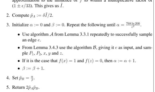
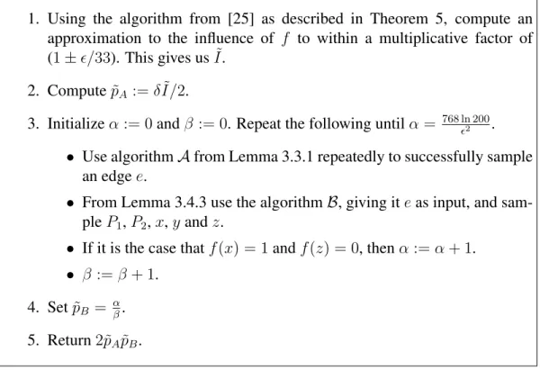
Algorithm for estimating noise sensitivity. (given oracle access to a monotone function 𝑓 : {0, 1}𝑛_{→ {0, 1}, and a parameter 𝜖)}

1. Using the algorithm from [25] as described in Theorem 5, compute an approximation to the influence of 𝑓 to within a multiplicative factor of (1 ± 𝜖/33). This gives us ˜𝐼.

2. Compute ˜𝑝𝐴:= 𝛿 ˜𝐼/2.

3. Initialize 𝛼 := 0 and 𝛽 := 0. Repeat the following until 𝛼 = 768 ln 200_𝜖2 .

∙ Use algorithm 𝒜 from Lemma 3.3.1 repeatedly to successfully sample an edge 𝑒.

∙ From Lemma 3.4.3 use the algorithm ℬ, giving it 𝑒 as input, and sam-ple 𝑃1, 𝑃2, 𝑥, 𝑦 and 𝑧.

∙ If it is the case that 𝑓 (𝑥) = 1 and 𝑓 (𝑧) = 0, then 𝛼 := 𝛼 + 1. ∙ 𝛽 := 𝛽 + 1.

4. Set ˜𝑝𝐵 = 𝛼_𝛽.

5. Return 2˜𝑝𝐴𝑝˜𝐵.

distinguish the case where the bias is 0 from the bias being 1/2𝑛 using a single query. Nevertheless, we show that for the most part, no algorithm for estimating the bias can do much better than the random sampling approach.

We construct two probability distributions 𝐷₁𝐵 and 𝐷₂𝐵 that are relatively hard to dis-tinguish but have drastically different biases. To create them, we fix some threshold 𝑙0 and

then construct a special monotone function 𝐹𝐵, which has the following two properties: (1) It has a high bias. (2) It equals to one on only a relatively small fraction of points on the level 𝑙0. We refer to functions satisfying (2) as “thin" functions. We will explain later how

to obtain such a function 𝐹𝐵. We pick a function from 𝐷𝐵₂ by taking 𝐹𝐵, randomly per-muting the indices of its input, and finally “truncating" it by setting it to one on all values

𝑥 for on levels higher than 𝑙0.

We form 𝐷𝐵₁ even more simply. We take the all-zeros function and truncate it at the same threshold 𝑙0. The threshold 𝑙0 is chosen in a way that this function in 𝐷𝐵1 has a

sufficiently small bias. Thus 𝐷𝐵₁ consists of only a single function.

The purpose of truncation is to prevent a distinguisher from gaining information by accessing the values of the function on the high-level vertices of the hypercube. Indeed, if there was no truncation, one could tell whether they have access to the all-zeros function by simply querying it on the all-ones input. Since 𝐹𝐵 is monotone, if it equals to one on at least one input, then it has to equal one on the all-ones input.

The proof has two main lemmas: The first one is computational and says that if 𝐹𝐵 is “thin" then 𝐷₁𝐵and 𝐷𝐵₂ are hard to reliably distinguish. To prove the first lemma, we show that one could transform any adaptive algorithm for distinguishing 𝐷𝐵₁ from 𝐷₂𝐵 into an algorithm that is just as effective, is non-adaptive and queries points only on the layer 𝑙0.

To show this, we observe that, because of truncation, distinguishing a function in 𝐷𝐵

2

from a function in 𝐷₁𝐵 is in a certain sense equivalent to finding a point with level at most

𝑙0 on which the given function evaluates to one. We argue that for this setting, adaptivity

does not help. Additionally, if 𝑥 ⪯ 𝑦 and both of them have levels at most 𝑙0 then, since 𝑓

is monotone, 𝑓 (𝑥) = 1 implies that 𝑓 (𝑦) = 1 (but not necessarily the other way around). Therefore, for finding a point on which the function evaluates to one, it is never more useful

to query 𝑥 instead of 𝑦.

Once we prove that no algorithm can do better than a non-adaptive algorithm that only queries points on the level 𝑙0, we use a simple union bound to show that any such algorithm

cannot be very effective for distinguishing our distributions.

Finally, to construct 𝐹𝐵, we need to show that there exist functions that are “thin" and simultaneously have a high bias. This is a purely combinatorial question and is proven in our second main lemma. We build upon Talagrand random functions that were first introduced in [26]. In [18] it was shown that they are very sensitive to noise, which was applied for property testing lower bounds [2]. A Talagrand random DNF consists of 2

√

𝑛

clauses of √𝑛 indices chosen randomly with replacement. We modify this construction

by picking the indices without replacement and generalize it by picking 2

√

𝑛_/𝑛𝐶2 _clauses,

where 𝐶2 is a non-negative constant. We show that these functions are “thin", so they are

appropriate for our lower bound technique.

“Thinness" allows us to conclude that 𝐷𝐵₁ and 𝐷₂𝐵 are hard to distinguish from each other. We then prove that they have drastically different biases. We do the latter by em-ploying the probabilistic method and showing that in expectation our random function has a large enough bias. We handle influence and noise sensitivity analogously, specifically by showing that that as we pick fewer clauses, the expected influence and noise sensitivity decrease proportionally. We prove this by dividing the points, where one of these random functions equals to one, into two regions: (i) the region where only one clause is true and (ii) a region where more than one clause is true. Roughly speaking, we show that the con-tribution from the points in (i) is sufficient to obtain a good lower bound on the influence and noise sensitivity.

1.4

Possibilities of improvement?

In [24] (which is the journal version of [25]), it was shown that using the chain decompo-sition of the hypercube, one can improve the run-time of the algorithm to 𝑂(︁

√

𝑛 𝜖2_{𝐼[𝑓 ]}

)︁

and also improve the required lower bound on 𝐼[𝑓 ] to be 𝐼[𝑓 ] ≥ exp(−𝑐1𝜖2𝑛 + 𝑐2log(𝑛/𝜖)) for

some constant 𝑐1 and 𝑐2(it was 𝐼[𝑓 ] ≥ 1/𝑛𝐶 for any constant 𝐶 in [25]). Additionally, the

algorithm itself was considerably simplified.

A hope is that techniques based on the chain decomposition could help improve the algorithm in Theorem 1. However, it is not clear how to generalize our approach to use these techniques, since the ascending-descending view is a natural way to express noise sensitivity in terms of random walks, and it is not obvious whether one can replace these walks with chains of the hypercube.

Chapter 2

Preliminaries

2.1

Definitions

2.1.1

Fundamental definitions and lemmas pertaining to the

hyper-cube.

Definition 1 We refer to the poset over {0, 1}𝑛 as the 𝑛-dimensional hypercube,

view-ing the domain as vertices of a graph, in which two vertices are connected by an edge if and only if the corresponding elements of {0, 1}𝑛 _{differ in precisely one index. For} 𝑥 = (𝑥1, . . . , 𝑥𝑛) and 𝑦 = (𝑦1, . . . , 𝑦𝑛) in {0, 1}𝑛, we say that𝑥 ⪯ 𝑦 if and only if for all 𝑖

in[𝑛] it is the case that 𝑥𝑖 ≤ 𝑦𝑖.

Definition 2 The level of a vertex 𝑥 on the hypercube is the hamming weight of 𝑥, or in other words number of1-s in 𝑥. We denote it by 𝐿(𝑥).

We define the set of edges that are in the same “layer" of the hypercube as a given edge:

Definition 3 For an arbitrary edge 𝑒 suppose 𝑒 = (𝑣1, 𝑣2) and 𝑣2 ⪯ 𝑣1. We denoteΛ𝑒 to

be the set of all edges𝑒′ = (𝑣₁′, 𝑣₂′), so that 𝐿(𝑣1) = 𝐿(𝑣′1) and 𝐿(𝑣2) = 𝐿(𝑣′2).

The size of Λ𝑒is 𝐿(𝑣1)

(︁ _𝑛

𝐿(𝑣1)

)︁

. The concept of Λ𝑒will be useful because we will deal with

paths that are symmetric with respect to change of coordinates, and these have an equal probability of hitting any edge in Λ𝑒.

As we view the hypercube as a graph, we will often refer to paths on it. By referring to a path 𝑃 we will, depending on the context, refer to its set of vertices or edges.

Definition 4 We call a path descending if for every pair of consecutive vertices 𝑣𝑖and𝑣𝑖+1,

it is the case that𝑣𝑖+1≺ 𝑣𝑖. Conversely, if the opposite holds and𝑣𝑖 ≺ 𝑣𝑖+1, we call a path

ascending. We consider an empty path to be vacuously both ascending and descending. We define the length of a path to be the number of edges in it, and denote it by |𝑃 |. We say we take a descending random walk of length 𝑤 starting at 𝑥, if we pick a uniformly random descending path of length𝑤 starting at 𝑥.

Descending random walks over the hyper-cube were used in an essential way in [25] and were central for the recent advances in monotonicity testing algorithms [5, 6, 15].

Lemma 2.1.1 (Hypercube Continuity Lemma) Suppose 𝑛 is a sufficiently large positive integer,𝐶1 is a constant and we are given𝑙1 and𝑙2 satisfying:

𝑛 2 − √︁ 𝐶1𝑛 log(𝑛) ≤ 𝑙1 ≤ 𝑙2 ≤ 𝑛 2 + √︁ 𝐶1𝑛 log(𝑛) If we denote 𝐶2 def = ₁₀√1

𝐶1, then for any 𝜉 satisfying 0 ≤ 𝜉 ≤ 1, if it is the case that

𝑙2− 𝑙1 ≤ 𝐶2𝜉

√︁ _𝑛

log(𝑛), then, for large enough𝑛, it is the case that 1 − 𝜉 ≤

(𝑛 𝑙1)

(𝑛 𝑙2)

≤ 1 + 𝜉

Proof: See Appendix C, Section C.2.

2.1.2

Fundamental definitions pertaining to Boolean functions

We define monotone functions over the 𝑛-dimensional hypercube:

Definition 5 Let 𝑓 be a function {0, 1}𝑛 _{→ {0, 1}}𝑛_{. We say that𝑓 is monotone if for any} 𝑥 and 𝑦 in {0, 1}𝑛,𝑥 ⪯ 𝑦 implies that 𝑓 (𝑥) ≤ 𝑓 (𝑦)

Influential edges, and influence of a function are defined as follows:

Definition 6 An edge (𝑥, 𝑦) in the hypercube is called influential if 𝑓 (𝑥) ̸= 𝑓 (𝑦). Addi-tionally, we denote the set of all influential edges in the hypercube as𝐸𝐼.

Definition 7 The influence of function 𝑓 : {0, 1}𝑛 → {0, 1}, denoted by 𝐼[𝑓 ] is:

𝐼[𝑓 ]= 𝑛 · Prdef 𝑥∈𝑅{0,1}𝑛,𝑖∈𝑅[𝑛][𝑓 (𝑥) ̸= 𝑓 (𝑥

⊕𝑖

)]

Where𝑥⊕𝑖is𝑥 with its 𝑖-th bit flipped.1 _{Equivalently, the influence is𝑛 times the probability}

that a random edge is influential. Since there are𝑛 · 2𝑛−1_{edges, then|𝐸}

𝐼| = 2𝑛−1𝐼[𝑓 ].

Definition 8 Let 𝛿 be a parameter and let 𝑥 be selected uniformly at random from {0, 1}𝑛_.

Let𝑧 ∈ {0, 1}𝑛be defined as follows:

𝑧𝑖 = ⎧ ⎪ ⎪ ⎨ ⎪ ⎪ ⎩ 𝑥𝑖 with probability1 − 𝛿 1 − 𝑥𝑖 with probability𝛿

We denote this distribution of𝑥 and 𝑧 by 𝑇𝛿. Then we define thenoise sensitivity of 𝑓 as:

𝑁 𝑆𝛿[𝑓 ]

def

= Pr(𝑥,𝑧)∈𝑅𝑇𝛿[𝑓 (𝑥) ̸= 𝑓 (𝑧)]

Observation 2.1.2 For every pair of vertices 𝑎 and 𝑏, the probability that for a pair 𝑥, 𝑧 drawn from𝑇𝛿, it is the case that(𝑥, 𝑧) = (𝑎, 𝑏), is equal to the probability that (𝑥, 𝑧) =

(𝑏, 𝑎). Therefore,

Pr[𝑓 (𝑥) = 0 ∧ 𝑓 (𝑧) = 1] = Pr[𝑓 (𝑥) = 1 ∧ 𝑓 (𝑧) = 0]

Hence:

𝑁 𝑆𝛿[𝑓 ] = 2 · Pr[𝑓 (𝑥) = 1 ∧ 𝑓 (𝑧) = 0]

2.1.3

Influence estimation.

To estimate the influence, standard sampling would require 𝑂(︁_{𝐼[𝑓 ]𝜖}𝑛 2

)︁

samples. However, from [25] we have:

1_{We use the symbol ∈}

𝑅to denote, depending on the type of object the symbol is followed by: (i) Picking

a random element from a probability distribution. (ii) Picking a uniformly random element from a set (iii) Running a randomized algorithm and taking the result.

Theorem 5 There is an algorithm that approximates 𝐼[𝑓 ] to within a multiplicative factor of(1 ± 𝜖) for a monotone 𝑓 : {0, 1}𝑛 _{→ {0, 1}. The algorithm requires that 𝐼[𝑓 ] ≥ 1/𝑛}𝐶′

for a constant 𝐶′ that is given to the algorithm. It outputs a good approximation with probability at least0.99 and in expectation requires 𝑂(︁

√

𝑛 log(𝑛/𝜖) 𝐼[𝑓 ]𝜖3

)︁

queries. Additionally, it runs in time polynomial in𝑛.

2.1.4

Bounds for 𝜖 and 𝐼[𝑓 ]

The following observation allows us to assume that without loss of generality 𝜖 is not too small. A similar technique was also used in [25].

Observation 2.1.3 When 𝜖 < 𝑂(√𝑛𝛿 log1.5(𝑛)) there is a simple algorithm that accom-plishes the desired query complexity of 𝑂(︁

√

𝑛𝛿 log1.5_(𝑛)

𝑁 𝑆𝛿[𝑓 ]𝜖3

)︁

. Namely, this can be done by the standard sampling algorithm that requires only 𝑂(︁_{𝑁 𝑆}1

𝛿[𝑓 ]𝜖2

)︁

samples. Thus, since we can handle the case when 𝜖 < 𝑂(√𝑛𝛿 log1.5(𝑛)), we focus on the case when 𝜖 ≥

𝐻√𝑛𝛿 log1.5(𝑛) ≥ 𝐻log√1.5𝑛

𝑛 , for any constant𝐻.

Additionally, throughout the paper whenever we need it, we will without loss of gener-ality assume that𝜖 is smaller than a sufficiently small positive constant.

We will also need a known lower bound on influence:

Observation 2.1.4 For any function 𝑓 : {0, 1}𝑛 → {0, 1} and 𝛿 ≤ 1/2 it is the case that:

𝑁 𝑆𝛿[𝑓 ] ≤ 𝛿𝐼[𝑓 ]

Therefore it is the case that𝐼[𝑓 ] ≥ _𝑛1𝐶.

A very similar statement is proved in [18] and for completeness we prove it in Appendix A.

Chapter 3

An improved algorithm for small 𝛿

In this section we give an improved algorithm for small 𝛿, namely 1/𝑛 ≤ 𝛿 ≤ 1/(√𝑛 log 𝑛).

We begin by describing the descending-ascending view on which the algorithm is based.

3.1

Descending-ascending framework

3.1.1

The descending-ascending process.

As we mentioned, it is be useful to view noise sensitivity in the context of the noise process in Figure 3.1.1. We will use the following notation for probabilities of various events: for an algorithm or a random process 𝑋 we will use the expression Pr𝑋[] to refer to the random

variables we defined in the context of this process or algorithm. It will often be the case that the same symbol, say 𝑥, will refer to different random random variables in the context of different random processes, so Pr𝑋[𝑥 = 1] might not be the same as Pr𝑌[𝑥 = 1].

By inspection, 𝑥 and 𝑧 are distributed identically in 𝐷 as in 𝑇𝛿. Therefore from

Obser-vation 2.1.2:

𝑁 𝑆𝛿[𝑓 ] = 2 · Pr𝐷[𝑓 (𝑥) = 1 ∧ 𝑓 (𝑧) = 0]

Observation 3.1.1 Since the function is monotone, if 𝑓 (𝑥) = 1 and 𝑓 (𝑧) = 0, then it has to be that𝑓 (𝑦) = 0.

Process 𝐷

1. Pick 𝑥 uniformly at random from {0, 1}𝑛_{. Let 𝑆}

0be the set of indexes 𝑖 for

which 𝑥𝑖 = 0, and conversely let 𝑆1 be the rest of indexes.

2. Phase 1: go through all the indexes in 𝑆1 in a random order, and flip each

with probability 𝛿. Form the descending path 𝑃1 from all the intermediate

results. Call the endpoint 𝑦.

3. Phase 2: start at 𝑦, and flip each index in 𝑆0with probability 𝛿. As before,

all the intermediate results form an ascending path 𝑃2, which ends in 𝑧.

4. Output 𝑃1, 𝑃2, 𝑥, 𝑦 and 𝑧.

Figure 3-1: The noise process (restated)

Now we define the probability that a Phase 1 path starting somewhere at level 𝑙 makes at least 𝑤 steps downwards:

Definition 9 For any 𝑙 and 𝑤 in [𝑛] we define 𝑄𝑙,𝑤as follows:

𝑄𝑙;𝑤 def = Pr𝐷[ ⃒ ⃒ ⃒𝑃1 ⃒ ⃒ ⃒≥ 𝑤|𝐿(𝑥) = 𝑙]

This notation is useful when one wants to talk about the probability that a path starting on a particular vertex hits a specific level.

3.1.2

Defining bad events

In this section, we give the parameters that we use to determine the lengths of our walks, as well as the “middle” of the hypercube.

Define the following values:

𝑡1 def = 𝜂1 √︁ 𝑛 log 𝑛 𝑡2 def = 𝑛𝛿(1 + 3𝜂2log 𝑛)

Here 𝜂1and 𝜂2are large enough constants. Taking 𝜂1 =

√

𝐶 +4 and 𝜂2 = 𝐶 +2 is sufficient

Informally, 𝑡1 and 𝑡2 have the following intuitive meaning. A typical vertex 𝑥 of the

hypercube has 𝐿(𝑥) between 𝑛/2 − 𝑡1 and 𝑛/2 + 𝑡1. A typical Phase 1 path from process

𝐷 will have length at most 𝑡2.

We define the “middle edges" 𝑀 as the following set of edges:

𝑀 def= {𝑒 = (𝑣1, 𝑣2) :

𝑛

2 − 𝑡1 ≤ 𝐿(𝑣2) ≤ 𝐿(𝑣1) ≤

𝑛

2 + 𝑡1} Denote by 𝑀 the rest of the edges.

We define two bad events in context of 𝐷, such that when neither of these events hap-pen, we can show that the output has certain properties. The first one happens roughly when 𝑃1(from 𝑥 to 𝑦, as defined by Process D) is much longer than it should be in

expecta-tion, and the second one happens when 𝑃1crosses one of the edges that are too far from the

middle of the hypercube, which could happen because 𝑃1 is long or because of a starting

point that is far from the middle. More specifically:

∙ 𝐸1 happens when both of the following hold (i) 𝑃1 crosses an edge 𝑒 ∈ 𝐸𝐼 and (ii)

denoting 𝑒 = (𝑣1, 𝑣2), so that 𝑣2 ⪯ 𝑣1, it is the case that 𝐿(𝑥) − 𝐿(𝑣1) ≥ 𝑡2.

∙ 𝐸2happens when 𝑃1 contains an edge in 𝐸𝐼 ∩ 𝑀 .

While defining 𝐸1 we want two things from it. First of all, we want its probability to be

upper-bounded easily. Secondly, we want it not to complicate the sampling of paths in Lemma 3.4.1. There exists a tension between these two requirements, and as a result the definition of 𝐸1is somewhat convoluted.

3.1.3

Defining 𝑝

, 𝑝

Ignoring the bad events, 𝑃𝐴is the probability that 𝑃1 hits an influential edge, and 𝑃𝐵is the

probability that given that 𝑃1 hits an influential edge 𝑃2 does not hit an influential edge.

From Observation (3.1.1), if and only if these two things happen, it is the case that 𝑓 (𝑥) = 1 and 𝑓 (𝑧) = 0. From this fact and the laws of conditional probabilities we have:

Pr𝐷[𝑓 (𝑥) = 1∧𝑓 (𝑧) = 0∧𝐸1∧𝐸2] = Pr𝐷[𝑓 (𝑥) = 1∧𝑓 (𝑦) = 0∧𝑓 (𝑧) = 0∧𝐸1∧𝐸2] = 𝑝𝐴𝑝𝐵

(3.1)

We can consider for every individual edge 𝑒 in 𝑀 ∩ 𝐸𝐼the probabilities:

𝑝𝑒 def= Pr𝐷[𝑒 ∈ 𝑃1∧ 𝐸1∧ 𝐸2]

𝑞𝑒

def

= Pr𝐷[𝑓 (𝑥) = 1 ∧ 𝑓 (𝑧) = 0|𝑒 ∈ 𝑃1 ∧ 𝐸1 ∧ 𝐸2] = Pr𝐷[𝑓 (𝑧) = 0|𝑒 ∈ 𝑃1∧ 𝐸1∧ 𝐸2]

The last equality is true because 𝑒 ∈ 𝑃1already implies 𝑓 (𝑥) = 1. Informally and ignoring

the bad events again, 𝑝𝑒 is the probability that 𝑓 (𝑥) = 1 and 𝑓 (𝑦) = 0 because 𝑃1 hits 𝑒

and not some other influential edge. Similarly, 𝑞𝑒is the probability 𝑓 (𝑥) = 1 and 𝑓 (𝑧) = 0

given that 𝑃1 hits specifically 𝑒.

Since 𝑓 is monotone, 𝑃1 can hit at most one influential edge. Therefore, the events of

𝑃1 hitting different influential edges are disjoint. Using this, Equation (3.1) and the laws of

conditional probabilities we can write:

𝑝𝐴 = ∑︁

𝑒∈𝐸𝐼∩𝑀

𝑝𝑒 (3.2)

Furthermore, the events that 𝑃1hits a given influential edge and then 𝑃2does not hit any are

also disjoint for different influential edges. Therefore, analogous to the previous equation we can write:

𝑝𝐴𝑝𝐵 = Pr𝐷[(𝑓 (𝑥) = 1) ∧ (𝑓 (𝑧) = 0) ∧ 𝐸1∧ 𝐸2] =

∑︁

𝑒∈𝐸𝐼∩𝑀

3.1.4

Bad events can be “ignored”

In the following proof, we will need to consider probability distributions in which bad events do not happen. For the most part, conditioning on the fact that bad events do not happen changes little in the calculations. In this subsection, we prove lemmas that allow us to formalize these claims.

The following lemma suggests that almost all influential edges are in 𝑀 .

Observation 3.1.2 It is the case that:

(︂

1 − 𝜖 310

)︂

|𝐸𝐼| ≤ |𝑀 ∩ 𝐸𝐼| ≤ |𝐸𝐼|

Proof: This is the case, because:

|𝑀 ∩ 𝐸𝐼| ≤ |𝑀 | ≤ 2𝑛𝑛 · 2 exp(−2𝜂12log(𝑛)) = 2𝑛−1· 4/𝑛2𝜂2 1−1 ≤ 2𝑛−1𝐼[𝑓 ]/𝑛 = |𝐸 𝐼|/𝑛 ≤ 𝜖 310|𝐸𝐼|

The second inequality is the Hoeffding bound, then we used Observations 2.1.4 and 2.1.3.

Lemma 3.1.3 We proceed to prove that ignoring these bad events does not distort our estimate for𝑁 𝑆𝛿[𝑓 ]. It is the case that:

𝑝𝐴𝑝𝐵 ≤ 1 2𝑁 𝑆𝛿[𝑓 ] ≤ (︂ 1 + 𝜖 5 )︂ 𝑝𝐴𝑝𝐵

Proof: See Appendix C, Section C.3.

3.2

Main lemmas

Here we prove the correctness and run-time of the main subroutines used in our algorithm for estimating noise sensitivity. For completeness, we will repeat all the algorithms.

3.3

Lemmas about descending paths hitting influential edges

Here we prove two lemmas that allow the estimation of the probability that a certain de-scending random walk hits an influential edge. As we mentioned in the introduction, ex-cept for the binary search step, the algorithm in Lemma 3.3.1 is similar to the algorithm in [25]. In principle, we could have carried out much of the analysis of the algorithm in Lemma 3.3.1 by referencing an equation in [25]. However, for subsequent lemmas, in-cluding Lemma 3.3.2, we build on the application of the Hypercube Continuity Lemma to the analysis of random walks on the hypercube. Thus, we give a full analysis of the algo-rithm in Lemma 3.3.1 here, in order to demonstrate how the Hypercube Continuity Lemma (Lemma 2.1.1) can be used to analyze random walks on the hypercube, before handling the more complicated subsequent lemmas, including Lemma 3.3.2.

Lemma 3.3.1 There exists an algorithm 𝒜 that samples edges from 𝑀 ∩ 𝐸𝐼 so that for

every two edges𝑒1and𝑒2in𝑀 ∩ 𝐸𝐼:

(︂ 1 − 𝜖 70 )︂ Pr𝑒∈𝑅𝒜[𝑒 = 𝑒2] ≤ Pr𝑒∈𝑅𝒜[𝑒 = 𝑒1] ≤ (︂ 1 + 𝜖 70 )︂ Pr𝑒∈𝑅𝒜[𝑒 = 𝑒2]

The probability that the algorithm succeeds is at least _𝑂(√ 1

𝑛 log1.5_{𝑛/𝐼[𝑓 ]𝜖)}. If it succeeds, the

algorithm makes 𝑂(log 𝑛) queries, and if it fails, it makes only 𝑂(1) queries. In either

case, it runs in time polynomial in𝑛.

Remark 3 Through the standard repetition technique, the probability of error can be de-creased to an arbitrarily small constant, at the cost of 𝑂(

√

𝑛 log1.5𝑛

𝐼[𝑓 ]𝜖 ) queries. Then, the

run-time still stays polynomial in𝑛, since 𝐼[𝑓 ] ≥ 1/𝑛𝐶_.

Remark 4 The distribution 𝒜 outputs is point-wise close to the uniform distribution over

𝑀 ∩ 𝐸𝐼. We will also obtain such approximations to other distributions in further lemmas.

Note that this requirement is stronger than closeness in𝐿1norm.

Algorithm 𝒜 (given oracle access to a monotone function 𝑓 : {0, 1}𝑛 → {0, 1} and a parameter 𝜖) 1. Assign 𝑤 = _3100𝜂𝜖 1 √︁ _𝑛 log 𝑛

2. Pick 𝑥 uniformly at random from {0, 1}𝑛.

3. Perform a descending walk 𝑃1 downwards in the hypercube starting at 𝑥.

Stop at a vertex 𝑦 either after 𝑤 steps, or if you hit the all-zeros vertex. Query the value of 𝑓 only at the endpoints 𝑥 and 𝑦 of this path.

4. If 𝑓 (𝑥) = 𝑓 (𝑦) output FAIL.

5. If 𝑓 (𝑥) ̸= 𝑓 (𝑦) perform a binary search on the path 𝑃1and find an influential

edge 𝑒𝑖𝑛𝑓.

6. If 𝑒𝑖𝑛𝑓 ∈ 𝑀 return 𝑒𝑖𝑛𝑓. Otherwise output FAIL.

Figure 3-2: Algorithm for sampling an influential edge (restated)

Note that 𝑃1 is distributed symmetrically with respect to a change of indexes. Pick an

arbitrary edge 𝑒0 in 𝑀 ∩ 𝐸𝐼 and let 𝑒0 = (𝑣1, 𝑣2), so 𝑣2 ⪯ 𝑣1. Recall that Λ𝑒0 was the set

of edges in the same “layer" of the hypercube and that |Λ𝑒0| equals 𝐿(𝑣1)

(︁ _𝑛

𝐿(𝑣1)

)︁

.

For any 𝑒′ in Λ𝑒0, 𝑒0 and 𝑒

′ _{are different only up to a permutation of indexes. This}

per-mutation of indexes induces a bijection between the set of descending paths going through

𝑒0 and those going through 𝑒′. Furthermore, since 𝑃1 is distributed symmetrically with

re-spect to a change of indexes, this bijection is between paths that have the same probability to be 𝑃1. Therefore, the probability that 𝑃1passes through 𝑒′ equals to the probability of it

passing through 𝑒0. Additionally, since 𝑃1 is descending it can cross at most one edge in

Λ𝑒0, which implies that the events of 𝑃1 crossing each of these edges are disjoint. Thus, we

can write: Pr𝒜[𝑒0 ∈ 𝑃1] = Pr𝒜[𝑃1∩ Λ𝑒0 ̸= ∅] 𝐿(𝑣1) (︁ _𝑛 𝐿(𝑣1) )︁

But 𝑃1 will intersect Λ𝑒0 if and only if 𝐿(𝑣1) ≤ 𝐿(𝑥) ≤ 𝐿(𝑣1) + 𝑤 − 1. This allows us to

above Λ𝑒0. Pr𝒜[𝑒0 ∈ 𝑃1] = ∑︀𝐿(𝑣1)+𝑤−1 𝑙=𝐿(𝑣1) 1 2𝑛 (︁_𝑛 𝑙 )︁ 𝐿(𝑣1) (︁ _𝑛 𝐿(𝑣1) )︁ (3.4)

Observation 2.1.3 allows us to lower-bound 𝜖 and argue that for sufficiently large 𝑛 we have: (︂ 1 − 𝜖 1300 )︂ ₂ 𝑛 ≤ 2 𝑛 1 1 + 2𝑡1/𝑛 ≤ 1 𝐿(𝑣1) ≤ 2 𝑛 1 1 − 2𝑡1/𝑛 ≤ (︂ 1 + 𝜖 1300 )︂ ₂ 𝑛 (3.5)

Since 𝑒 ∈ 𝑀 , it is the case that 𝑛₂− 𝑡1 ≤ 𝐿(𝑣2) ≤ 𝐿(𝑣1) ≤ 𝑛₂ + 𝑡1. This allows us to use

Lemma 2.1.1 and deduce that 1 − 𝜖/310 ≤ (︁𝑛_𝑙)︁/(︁_𝐿(𝑣𝑛

1)

)︁

≤ 1 + 𝜖/310. This and Equation (3.5) allow us to approximate Pr𝒜[𝑒0 ∈ 𝑃1] in Equation (3.4) the following way:

(︂ 1 − 𝜖 150 )︂ _𝑤 𝑛2𝑛−1 ≤ Pr𝒜[𝑒0 ∈ 𝑃1] ≤ (︂ 1 + 𝜖 150 )︂ _𝑤 𝑛2𝑛−1 (3.6)

The algorithm outputs an influential edge if and only if 𝑃1hits an influential edge in 𝑀 ∩𝐸𝐼.

At the same time, these events corresponding to different edges in 𝑀 ∩𝐸𝐼are disjoint since 𝑃1 can hit only at most one influential edge. This together with Bayes rule allows us to

express the probability that the algorithm outputs 𝑒0, conditioned on it succeeding:

Pr𝑒∈𝑅𝒜[𝑒 = 𝑒0] = Pr𝒜[𝑒𝑖𝑛𝑓 = 𝑒0] = Pr𝒜 ⎡ ⎣𝑒₀ ∈ 𝑃₁ ⃒ ⃒ ⃒ ⃒ ⃒ ⋁︁ 𝑒′_{∈𝑀 ∩𝐸} 𝐼 (𝑒′ ∈ 𝑃1) ⎤ ⎦= Pr𝒜[𝑒0 ∈ 𝑃1] Pr𝒜 [︁ ⋁︀ 𝑒′_{∈𝑀 ∩𝐸} 𝐼(𝑒 ′ _{∈ 𝑃} 1) ]︁ (3.7)

Substituting Equation (3.7) into Equation (3.6) we get:

(︂ 1 − 𝜖 150 )︂ _𝑤 𝑛2𝑛−1 · Pr𝒜 ⎡ ⎣ ⋁︁ 𝑒1∈𝑀 ∩𝐸𝐼 (𝑒1 ∈ 𝑃1) ⎤ ⎦≤ Pr_𝑒∈𝑅𝒜[𝑒 = 𝑒0] ≤ (︂ 1 + 𝜖 150 )︂ 𝑤 𝑛2𝑛−1 · Pr𝒜 ⎡ ⎣ ⋁︁ 𝑒1∈𝑀 ∩𝐸𝐼 (𝑒1 ∈ 𝑃1) ⎤ ⎦

the resulting inequalities gives us:

1 − 𝜖/150

1 + 𝜖/150Pr𝑒∈𝑅𝒜[𝑒 = 𝑒2] ≤ Pr𝑒∈𝑅𝒜[𝑒 = 𝑒1] ≤

1 + 𝜖/150

1 − 𝜖/150Pr𝑒∈𝑅𝒜[𝑒 = 𝑒2]

From this, the correctness of the algorithm follows. In case of failure, it makes 𝑂(1) queries and in case of success, it makes 𝑂(log 𝜖 + log(𝑛/ log 𝑛)) = 𝑂(log 𝑛) queries, because of the additional binary search. In either case, the run-time is polynomial.

Now, regarding the probability of success, note that the events of 𝑃1 crossing

differ-ent edges in 𝐸𝐼 ∩ 𝑀 are disjoint since the function is monotone. Therefore, we can sum

Equation (3.6) over all edges in 𝑀 ∩ 𝐸𝐼 and get that the probability of success is at least

Θ(︁|𝐸𝐼∩𝑀 |𝑤

𝑛2𝑛−1

)︁

. Applying Lemma 3.1.2 and substituting 𝑤, the inverse of the success proba-bility is: 𝑂 (︃ 𝑛2𝑛−1 |𝐸𝐼∩ 𝑀 |𝑤 · log 𝑛 )︃ = 𝑂 (︃ 𝑛 𝐼[𝑓 ]𝑤 · log 𝑛 )︃ = 𝑂 (︃ log1.5(𝑛)√𝑛 𝐼[𝑓 ]𝜖 )︃

The following lemma, roughly speaking, shows that just as in previous lemma, the probability that 𝑃1 in 𝐷 hits an influential edge 𝑒 does not depend on where exactly 𝑒 is,

as long as it is in 𝑀 ∩ 𝐸𝐼. The techniques we use are similar to the ones in the previous

lemma and it follows the same outline. However here we encounter additional difficulties for two reasons: first of all, the length of 𝑃1 is not fixed, but it is drawn from a probability

distribution. Secondly, this probability distribution depends on the starting point of 𝑃1.

Note that unlike what we have in the previous lemma, here 𝑃1comes from the

ascending-descending view of noise sensitivity.

Lemma 3.3.2 For any edge 𝑒 ∈ 𝑀 ∩ 𝐸𝐼it is the case that:

(︂ 1 − 𝜖 310 )︂ _𝛿 2𝑛 ≤ 𝑝𝑒 ≤ (︂ 1 + 𝜖 310 )︂ _𝛿 2𝑛

the proof of Lemma 3.3.1. We get: 𝑝𝑒= Pr𝐷[(𝑒 ∈ 𝑃1) ∧ 𝐸1∧ 𝐸2] = Pr𝐷[(𝑒 ∈ 𝑃1) ∧ 𝐸1] = Pr𝐷[(𝑒 ∈ 𝑃1) ∧ (𝐿(𝑥) − 𝐿(𝑣1) < 𝑡2)] = Pr𝐷[(𝑃1∩ Λ𝑒 ̸= ∅) ∧ (𝐿(𝑥) − 𝐿(𝑣1) < 𝑡2)] 𝐿(𝑣1) (︁ _𝑛 𝐿(𝑣1) )︁

Above we did the following: Recall that 𝐸2is the event that 𝑃1crosses an edge in 𝐸𝐼∩ 𝑀 .

The first equality is true because 𝑒 ∈ 𝐸𝐼∩ 𝑀 and 𝑃1can cross at most one influential edge,

which implies that 𝐸2 cannot happen. For the second equality we substituted the definition

of 𝐸1. For the third equality we used the symmetry of 𝐷 with respect to change of indexes

just as in the proof of Lemma 3.3.1.

Recall that we defined:

𝑄𝑙;𝑤 def = Pr𝐷[ ⃒ ⃒ ⃒𝑃1 ⃒ ⃒ ⃒≥ 𝑤|𝐿(𝑥) = 𝑙]

This allows us to rewrite:

𝑝𝑒 = ∑︀𝑡2 𝑖=1₂1𝑛 (︁ _𝑛 𝐿(𝑣1)+𝑖−1 )︁ 𝑄𝐿(𝑣1)+𝑖−1;𝑖 𝐿(𝑣1) (︁ _𝑛 𝐿(𝑣1) )︁ (3.8)

Above we just looked at each of the layers of the hypercube and summed the contributions from them.

To prove a bound on 𝑝𝑒 we will need a bound on 𝑡2. Observation 2.1.3 implies that for

any 𝐻 we can assume that√𝑛𝛿 ≤ _{𝐻 log}𝜖1.5_𝑛 using which we deduce

𝑡2 = 𝑛𝛿(1 + 3𝜂2log(𝑛)) ≤ 4𝜂2𝑛𝛿 log(𝑛) ≤ 4𝜂2𝜖 𝐻 √︃ 𝑛 log 𝑛

Furthermore, we will need a bound on the binomial coefficients in Equation (3.8). By picking 𝐻 to be a large enough constant, this allows us to use Lemma 2.1.1 to bound the

ratios of the binomial coefficients. For any 𝑖 between 1 and 𝑡2inclusive: 1 − 𝜖 1300 ≤ (︁ _𝑛 𝐿(𝑣1)+𝑖−1 )︁ (︁ _𝑛 𝐿(𝑣1) )︁ ≤ 1 + 𝜖 1300 (3.9)

Equation (3.5) is valid in this setting too. Substituting Equation (3.5) together with Equa-tion (3.9) into EquaEqua-tion (3.8) we get:

(︂ 1 − 𝜖 630 )︂ ₁ 𝑛2𝑛−1 𝑡2 ∑︁ 𝑖=1 𝑄𝐿(𝑣1)+𝑖−1;𝑖 ≤ 𝑝𝑒≤ (︂ 1 + 𝜖 630 )︂ ₁ 𝑛2𝑛−1 𝑡2 ∑︁ 𝑖=1 𝑄𝐿(𝑣1)+𝑖−1;𝑖 (3.10)

Observe that a vertex on the level 𝑙 + 1 has more ones than a vertex on level 𝑙. So for a positive integer 𝑤, the probability that at least 𝑤 of them will flip is larger. Therefore,

𝑄𝑙,𝑤 ≤ 𝑄𝑙+1,𝑤. This allows us to bound:

𝑡2 ∑︁ 𝑖=1 𝑄𝐿(𝑣1);𝑖≤ 𝑡2 ∑︁ 𝑖=1 𝑄𝐿(𝑣1)+𝑖−1;𝑖 ≤ 𝑡2 ∑︁ 𝑖=1 𝑄𝐿(𝑣1)+𝑡2−1;𝑖 (3.11)

Then, using Observation 2.1.3:

𝑡2 ∑︁ 𝑖=1 𝑄𝐿(𝑣1)+𝑡2−1;𝑖 ≤ 𝑛 ∑︁ 𝑖=1 𝑄𝐿(𝑣1)+𝑡2−1;𝑖 = 𝐸𝐷[𝐿(𝑥) − 𝐿(𝑦)|𝐿(𝑥) = 𝐿(𝑣1) + 𝑡2 − 1] = 𝛿(𝐿(𝑣1) + 𝑡2− 1) ≤ 𝛿(𝑛/2 + 𝑡1+ 𝑡2) ≤ (︂ 1 + 𝜖 630 )︂_𝑛𝛿 2 (3.12)

Now, we bound from the other side:

𝑡2 ∑︁ 𝑖=1 𝑄𝐿(𝑣1);𝑖= 𝑛 ∑︁ 𝑖=1 𝑄𝐿(𝑣1);𝑖− 𝑛 ∑︁ 𝑖=𝑡2+1 𝑄𝐿(𝑣1);𝑖≥ 𝑛 ∑︁ 𝑖=1 𝑄𝐿(𝑣1);𝑖− 𝑛 · 𝑄𝐿(𝑣1);𝑡2 (3.13)