Algorithms and lower bounds in finite automata size complexity

(1)

ALGORITHMS AND LOWER BOUNDS

IN FINITE AUTOMATA SIZE COMPLEXITY

by

CHRISTOS KAPOUTSIS

B.S. Computer Science, Aristotle University of Thessaloniki, Greece, 1997 M.S. Logic and Algorithms, Capodistrian University of Athens, Greece, 2000

M.S. Computer Science, Massachusetts Institute of Technology, 2004

Submitted to the Department of Electrical Engineering and Computer Science in partial fulfillment of the requirements for the degree of

DOCTOR OF PHILOSOPHY

at the Massachusetts Institute of Technology, June 2006

Signature of author:

Department of Elect ical ngineering and Computer Science May 5, 2006

Michael Sipser Professpr of Applied Mathematics Thesw Supervisor

Arthur C. Smith Professor of Electrical Engineering Graduate Officer, EECS Graduate Office Accepted by: -Certified by: MASSACHUSETTS 1N4TMUTI OF TECHNOLOGY

NOV

j

2 2006

LIBRARIES

(2)

(3)

ALGORITHMS AND LOWER BOUNDS

IN FINITE AUTOMATA SIZE COMPLEXITY

by

CHRISTOS KAPOUTSIS

Submitted to the Department of Electrical Engineering and Computer Science in partial fulfillment of the requirements for the degree of Doctor of Philosophy.

Abstract

In this thesis we investigate the relative succinctness of several types of finite automata, focusing mainly on the following four basic models: one-way

determinis-tic (1DFAS), one-way nondeterministic (1NFAs), two-way deterministic (2DFAs), and two-way nondeterministic (2NFAs).

First, we establish the exact values of the trade-offs for all conversions from two-way to one-way automata. Specifically, we prove that the functions

n(n"

- (n - 1)"), n1

I

(n)(n) (2' - 1)j,

(2n")

return the exact values of the trade-offs from 2DFAs to 1DFAs, from 2NFAs to 1DFAs, and from 2DFAs or 2NFAs to 1NFAs, respectively.

Second, we examine the question whether the trade-offs from INFAs or 2NFAs to 2DFAs are polynomial or not. We prove two theorems for liveness, the complete problem for the conversion from 1NFAs to 2DFAs. We first focus on moles, a restricted class of 2NFAs that includes the polynomially large 1NFAs which solve liveness. We prove that, in contrast, 2DFA moles cannot solve liveness, irrespective of size. We then focus on sweeping 2NFAs, which can change the direction of their input head only on the end-markers. We prove that all sweeping 2NFAs solving the complement of liveness are of exponential size. A simple modification of this argument also proves that the trade-off from 2DFAs to sweeping 2NFAs is exponential.

Finally, we examine conversions between two-way automata with more than one head-like devices (e.g., heads, linearly bounded counters, pebbles). We prove that, if the automata of some type A have enough resources to (i) solve problems that no automaton of some other type B can solve, and (ii) simulate any unary 2DFA that has additional access to a linearly-bounded counter, then the trade-off from automata of type A to automata of type B admits no recursive upper bound.

(4)

(5)

-Introduction

The main subject of this thesis is the 2D vs. 2N problem, a question on the power of nondeterminism in two-way finite automata. We start by defining it, explaining the motivation for its study, and describing our progress against it.

1. The 2D vs. 2N Problem

A two-way deterministic finite automaton (2DFA) is the machine that we get from the common one-way deterministic finite automaton (1DFA) when we allow its input head to move in both directions; equivalently, this is the machine that we get from the common single-tape deterministic Turing machine (DTM) when we do not allow its input head to write on the input tape. The nondeterministic version of a 2DFA is simply called two-way nondeterministic finite automaton (2NFA) and, as usual, is the machine that we get by allowing more than one options at each step and acceptance by any computation branch. The 2D vs. 2N question asks whether 2NFAs can be strictly more efficient than 2DFAs, in the sense that there is a problem for which the best 2DFA algorithm is significantly worse than the best 2NFA one.

Of course, to complete the description of the question, we need to explain how we measure the efficiency of an algorithm on a two-way finite automaton. It is easy to check that, with respect to the length of its input, every algorithm of this kind uses zero space and at most linear time. Therefore, the time and space measures-our typical criteria for algorithmic efficiency on the full-fledged Turing machine-are of little help in this context. Instead, we focus on the size of the program that encodes this algorithm, namely the size of the transition function of the corresponding two-way finite automaton. In turn, a good measure for this size is simply the automaton's number of states.

So, the 2D vs. 2N question asks whether there is a problem that, although it can be solved both by 2DFAs and by 2NFAs, the smallest possible 2DFA for it (i.e., the 2DFA that solves it with the fewest possible states) is still significantly larger than the smallest possible 2NFA for it. To fully understand the question, two additional clarifications are needed.

First, it is well-known that the problems that are solvable by 2DFAs are exactly those described by the regular languages, and that the same is true for 2NFAs [53. Hence, efficiency considerations aside, the two types of automata have the same power-in the same way that 1DFAs or DTMs have the same power with their non-deterministic counterparts. Therefore, the above reference to problems that "can be solved both by 2DFAs and by 2NFAs" is a reference to exactly the regular problems. Second, although we explained that efficiency is measured with respect to the number of states, we still have not defined what it means for the number of states in one automaton to be "significantly larger" than the number of states in another one. The best way to clarify this aspect of the question is to give a specific example.

(8)

INTRODUCTION

Consider the problem in which we are given a list of subsets of {0, 1,. .. , n - 1} and we are asked whether this list can be broken into sublists so that the first set of every sublist contains the number of sets after it [51]. More precisely, the problem is defined on the alphabet An :='P({0, 1,.. .,

n

- 1}) of all sets of numbers smaller than n. A string a0a, - --al over this alphabet is a block if its first symbol is a set that contains the number of symbols after it, that is, if ao E 1. The problem consists in determining whether a given string over

An

can be written as a concatenation of blocks. For example, for n = 8 and for the string

{ 1,2,4}0{4}{0,4}{2,4,6}{4}{4,6}0{3,6}0{2,4}{5,7}{0,3}{4,7}0{4}@{4}{0,1} {2,5,6}{1}

the answer should be "yes", since this is the concatenation of the substrings

{1,2,4}0{4} {0,4}{2,4,6}{4}{4,6}0 {3,6}0{2,4}{5,7} {0,3} {4,7}0{4}0{4}{0,1}{2,5,6}{1} where the first set in each substring indeed contains the number of sets after it in the same substring, as indicated by boldface. In contrast, for the string

{1,2,7}{4}{5,6}0{3,6}{2,4,6}

the answer should be "no", as there is obviously no way to break it into blocks. Is there a 2DFA algorithm for this problem? Is there a 2NFA algorithm? Indeed, the problem is regular. The best 2NFA algorithm for it is a rather obvious one:

We scan the list of sets from left to right. At the start of each block, we read the first set. If it is empty, we just hang (in this branch

of the computation). Otherwise, we nondeterministically select from this set the correct number of remaining sets in the block. We then consume as many sets, counting from that number down. When the count reaches 0, we know the block is over and a new one is about to start. In the end, we accept if the list and our last count-down finish simultaneously.

It is easy to see that this algorithm can be implemented on a 2NFA (which does not actually use its bidirectionality) with exactly 1 state per possible value of the counter, for a total number of n states. As for a 2DFA algorithm, here is the best known one:

We scan the list of sets from left to right. At each step, we remem-ber all possibilities about how many more sets there are in the most recent block. (E.g., right after the first set, every number in it is a possibility.) After reading each set, we decrease each possibility by 1, to account for the set just consumed; if a possibility becomes 0, we replace it by all numbers of the next set. If at any point the set of possibilities gets empty, we just hang. Otherwise, we eventually reach the end of the list. There, we check whether 0 is among the possibilities. If so, we accept.

Easily, this algorithm can be implemented on a 2DFA (which does not actually use its bidirectionality) that has exactly 1 state per possible non-empty1 set of possibilities, for a total number of 2" - 1 states. Overall, we see that the difference in size between the automata implementing the two algorithms is exponential. Such a difference, we surely want to call "significant".

INote that a 2DFA is allowed to reject by just hanging anywhere along its input. Without this freedom, the number of states required to implement our algorithm would actually be 2'.

(9)

2. MOTIVATION

At this point, after the above clarifications, we may want to restate the 2D vs. 2N question as the question whether there exists a regular problem for which the small-est possible 2DFA is still super-polynomially larger than the smallsmall-est possible 2NFA. However, a further clarification is due.

Given any fixed regular problem, the sizes of the smallest possible 2DFA and the smallest possible 2NFA for it are nothing more than just two numbers. So, asking whether their difference is polynomial or not makes little sense. What the previous example really describes is a family of regular problems IH = (ITn),,

one for each natural value of n; then, a family of 2NFAs N = (N,)n o which solve these problems and whose sizes grow linearly in n; and, finally, a family of 2DFAs

D = (Dn),o which also solve these problems and whose sizes grow exponentially

in n. Therefore, our reference to "the difference in size between the automata" was really a reference to the difference in the rate of growth of the sizes of the automata in the two families. It is this difference that can be characterized as polynomial or not. Naturally, we decide to call it significant if one of the two rates can be bounded by a polynomial but the other one cannot.

So, the 2D vs. 2N question asks whether there exists a family of regular problems such that the family of the smallest 2NFAs that solve them have sizes that grow polynomially in n, whereas the family of the smallest 2DFAs that solve them have sizes that grow super-polynomially in n. Equivalently, the question is whether there

exists a family of regular problems that can be solved by a polynomial-size family

of 2NFAs but no polynomial-size family of 2DFAs. With this clarification, we are

ready to explain the name "2D vs. 2N". We define 2D as the class of families of regular problems that can be solved by polynomial-size families of 2DFAs, and 2N as the corresponding class for 2NFAs [48]. Under these definitions, we obviously have 2D C 2N, and the question is whether 2D and 2N are actually different. Observe how the nature of the question resembles both circuit and Turing machine complexity: like circuits, we are concerned with the rate of growth of size in families of programs; unlike circuits and like Turing machines, each program in a family can work on inputs of any length.

Concluding this description of the problem, let us also remark that its formu-lation in terms of families is not really part of our every-day vocabulary in working on the problem. Instead, we think and speak as if n were a built-in parameter of our world, so that only the n-th members of the three families (of problems, of 2NFAs, and of 2DFAs) were visible. Under this pretense, the 2D vs. 2N question asks

whether there is a regular problem that can be solved by a polynomially large 2NFA but no polynomially large 2DFA-and it is redundant to mention what parameter "polynomially large" refers to. In addition, we also use "small" as a more intuitive substitute for "polynomially large", and drop the obviously redundant character-ization "regular". So, the every-day formulation of the question is whether there exists a problem that can be solved by a small 2NFA but no small 2DFA. Throughout

this thesis, we will occasionally be using this kind of talk, with the understanding that it is a substitute for its formal interpretation in terms of families.

2. Motivation

Our motivation for studying the 2D vs. 2N question comes from two distinct sources: the theory of computational complexity and the theory of descriptional

complexity. We discuss these two different contexts separately.

(10)

INTRODUCTION

2.1. Computational complexity. From the perspective of computational complexity, the 2D vs. 2N question falls within the general major goal of understand-ing the power of nondeterminism. For certain computational models and resources, this quest has been going on for more than four decades now. Of course, the most important (and correspondingly famous) problem of this kind is P vs. NP, defined on the Turing machine and for time which is bounded by some polynomial of the length of the input. The next most important question is probably L vs. NL, also defined on the Turing machine and for space which is bounded by the logarithm of some polynomial of the length of the input.

It is perhaps fair to say that our progress against the core of these problems

has been slow. Although our theory is constantly being enriched with new concepts

and new connections between the already existing ones, major advances of our understanding are rather sparse. At the same time, the common conceptual origin as well as certain combinatorial similarities between these problems has led some to suspect that essentially the same elusive idea lies at the core of all problems of

this kind. In particular, the suspicion goes, this idea may be independent of the

specifics of the underlying computational model and resource.

In this context, a possibly advantageous approach is to focus on weak models of computation. The simple setting provided by these models allows us to work closer to the set-theoretic objects that are produced by their computations. This serves us in two ways. First, it obviously helps our arguments become cleaner and more robust. Second, it helps our reasoning become more objective, by neutralizing our often misleading algorithmic intuitions about what a machine may or may not do. The only problem with this approach is that it may very well lead us to models of computation that are too weak to be relevant. In other words, some of these models are obviously not rich enough to involve ideas of the kind that we are looking for. We should therefore be careful to look for evidence that indeed such ideas are present. We believe that the 2D vs. 2N question passes this test, and we explain why. 2.1-I. Robustness. One of the main reasons why problems like P vs. NP and L vs. NL are so attractive is their robustness. The essence of each question remains the same under many different variations of the mathematical definitions of the model and/or the resource. It is only on such stable grounds that the theoretical framework around each question could have been erected, with the definition of the

classes of problems that can be solved in each case (P, NP, L, NL) and the identifica-tion of complete problems for the nondeterministic classes, that allowed for a more tangible reformulation of the original question (is satisfiability in P? is connectivity in L?). The coherence and richness of these theories further enhance our confi-dence that they indeed describe important high-level questions about the nature of computation, as opposed to technical low-level inquiries about the peculiarities of particular models.

The 2D vs. 2N problem is also robust. Its resolution is independent of all rea-sonable variations of the definition of the two-way finite automaton and/or the size measure, including changes in the conventions for accepting and rejecting, for end-marking the input, for moving the head; changes in the size of the alphabet, which may be fixed to binary; changes in the size measure, which may include the number of transitions or equal the length of some fixed binary encoding. It is on this stable ground that the classes 2D and 2N have been defined. In addition, 2N-complete (families of) problems have been identified [48], allowing more concrete forms of

(11)

2. MOTIVATION

the question. Overall, there is no doubt that in this case, too, our investigations are beyond technical peculiarities and into the high-level properties of computation.

2.1-II. Hardness. A second important characteristic of problems like P vs. NP and L vs. NL that contributes to their popularity is their hardness. Until today, a long list of people that cared about these problems have tried to attack them from several different perspectives and with several different techniques. Their limited success constitutes significant evidence that, indeed, answering these questions will require a deeper understanding of the combinatorial structure of computation. In this sense, the answer is likely to be highly rewarding.

In contrast, the 2D vs. 2N problem can boast no similar attention on the part of the community, as it has never attracted the efforts of a large group of researchers. However, it does belong to the culture of this same community and several of its members have tried to attack it or problems around it, with the same limited success. In this sense, it is again fair to predict that the answer to this question will indeed involve ideas which are deep enough to be significantly rewarding.

2.1-III. Surprising conjecture. If we open a computational complexity

text-book, we will probably find P defined as the class of problems that can be solved by polynomial-time Turing machines, and NP as the class of problems that can be solved by the same machines when they are enhanced with the ability to make non-deterministic choices. Then, we will probably also find a discussion of the standard conjecture that P

$

NP, justified by the well-known compelling list of pragmatic and philosophical reasons.

In this context, the conjecture does not sound surprising at all. There is cer-tainly nothing strange with the enhanced machines being strictly more powerful than the original, non-enhanced ones. They start already as powerful, and then the magical extra feature of nondeterminism comes along: how could this result in nothing new? But the conjecture does describe a fairly intriguing situation.

First, if we interpret the conjecture in the context of the struggle of fast deter-ministic algorithms to subdue fast nondeterdeter-ministic ones, it says that a particular nondeterministic Turing machine using just one tape and only linear time [37] can actually solve a problem that defies all polynomial-time multi-tape deterministic Turing machines, irrespective of the degree of the associated polynomial and the number of tapes. In other words, the claim is that nondeterministic algorithms can

beat deterministic ones even with minimal use of the rest of their abilities. This is

an aspect of the P

#

NP conjecture that our definitions do not highlight.

Second, if we interpret the conjecture in the context of the struggle of fast deterministic algorithms to solve a specific NP-complete problem, it says that the fastest way to check whether a propositional formula is satisfiable is essentially to try all possible assignments. Although this matches with our experience in one sense (in the simple sense that we have no idea how to do anything faster in general), it also seriously clashes with our experience in another sense, equally important: it claims that the obvious, highly inefficient solution is also the optimal one. This is in contrast with what one would first imagine, given that optimality is almost always associated with high sophistication.

Similar comments are valid for L vs. NL. The standard conjecture that L

f

NL asserts that a particular nondeterministic finite automaton with a small bunch of states and just two heads that only move one-way [57] can actually solve a problem that defies all deterministic multi-head two-way finite automata, irrespective of

(12)

INTRODUCTION

their number of states and heads. At the same time, it claims that the most space-economical method of checking connectivity is essentially the one by Savitch, a fairly non-trivial algorithm which nevertheless still involves several natural choices (e.g., recursion) and lacks the high sophistication that we usually expect in optimality.

Similarly to P vs. NP and L Vs. NL, the conjecture for the 2D vs. 2N problem is again that 2D

#

2N. Moreover, two stronger variants of it have also been proposed. First, it is conjectured that 2NFAs can be exponentially smaller than 2DFAs even when they never move their head to the left. In other words, it is suggested that even one-way nondeterministic finite automata (INFAs) can be exponentially smaller than 2DFAs. (Note the similarity with the version of L k NL mentioned above, where the nondeterministic automaton need only move its heads one-way to beat all two-way multi-head deterministic ones.) So, once more we have an instance of the claim that nondeterministic algorithms can beat deterministic ones with minimal use of the rest of their abilities.

Second, it is even conjectured that this alleged exponential difference in size

between 1NFAs and 2DFAs covers the entire gap from n to 2' - 1 which is known to

exist between

1NFAs

and 1DFAs [35]2 In other words, according to this conjecture, a 2DFA trying to simulate a

1NFA

may as well drop its bidirectionality, since it is going to be totally useless: its optimal strategy is going to be the well-known brute-force one-way deterministic simulation [47]. So, once more we have an instance of the claim that the obvious, highly inefficient solution is also the optimal one.3

For a concrete example of what all this means, recall the problem that we described early in this introduction (page 8). Remember that we presented it as a problem that is solvable by small 2NFAs but is conjectured to require large 2DFAs. Notice that the best 2NFA algorithm presented there is actually one-way, namely a 1NFA. So, if the conjecture about this problem is true, then 2NFAs can indeed beat 2DFAs, and they can do so without using their bidirectionality. Also notice that the best known 2DFA for that problem is one-way, too. In fact, it is simply the brute-force 1DFA simulation of the INFA solver. So, if this is really the smallest

2DFA for the problem, then indeed the optimal way of simulating the hardest 2NFA is the obvious, highly inefficient one.

In total, interpreting the questions on the power of nondeterminism (P vs. NP, L vs. NL) as a contest between deterministic and nondeterministic algorithms, our conjectures claim that nondeterministic algorithms can win with one hand behind their back; and then, the best that deterministic algorithms can do in their defeat to minimize their losses is essentially not to think. This is a counter-intuitive claim, and our conjectures for 2D vs. 2N make this same claim, too.

2.1-IV. A mathematical connection. Of the similarities described above be-tween 2D vs. 2N and the more important questions on the power of nondeterminism, none is mathematical. However, a mathematical connection is known, too. As ex-plained in [3], if we can establish that 2D

#

2N using only "short" strings, then we

2

As with 2DFAS (cf. Footnote 1 on _{page 8), a iDFA is allowed to reject by just hanging anywhere} along its input. Without this freedom, the gap would actually be from n to 2".

3

Note that, contrary to the strong versions of P O NP and L A NL mentioned above [37, 571,

the two conjectures mentioned in these two last paragraphs may be strictly stronger than 2D = 2N. It may very well be that 1NFAs cannot be exponentially smaller than 2DFAs, but 2NFAs can (it is known that 2NFAs can be exponentially smaller than 1NFAs). Moreover, even if INFAs can be exponentially smaller than 2DFAs, it may very well be that this exponential gap is smaller than the gap from n to 2' - 1.

(13)

2. MOTIVATION

would also have a proof that L / NL. To describe this implication more carefully, we need to first discuss how a proof of 2D 2N may actually proceed.

To prove the conjecture, we need to start with a 2N-complete family of regular problems H = (HI),;>o, and prove that it is not in 2D. That is, we must prove that for any polynomial-size family of 2DFAs D = (D ),>o there exists an n which is

bad, in the sense that D, does not solve 17'. Now, two observations are due: * To prove that some n is bad, we need to find a string w, that "fools" Ds, in

the sense that w, E H, but D, rejects w., or w,, 17, but D. accepts w,. * Every D has a bad n iff every D has infinitely many bad n. This is true

because, if a polynomial-size family D has only finitely many bad n, then replacing the corresponding D, with correct automata of any size would result in a new family which is still polynomial-size and has no bad n. Hence, proving the conjecture amounts to proving that, for any polynomial-size family D of 2DFAs for H, there is a family of strings w = (w,);>o such that, for infinitely many n, the input w, fools D,.

Now, the connection with L vs. NL says the following: if we can indeed find such a proof and in addition manage to guarantee that the lengths of the strings in w are bounded by some polynomial of n, then L

#

NL.

There is no doubt that this connection increases our confidence in the relevance of the 2D vs. 2N problem to the more important questions on the power of nonde-terminism. However, its significance should not be over-estimated. First, the two

problems may very well be resolved independently. On one hand, if 2D = 2N then the connection is irrelevant, obviously. On the other hand, if 2D / 2N then our tools for short strings are so much weaker than our tools for long strings, that it is hard to imagine us arriving at a proof that uses only short strings before actually having a proof that uses long ones. Second, and perhaps most importantly, ideas do not need

mathematical connections to transcend domains. In other words, an idea that works

for one type of machines may very well be applicable to other types of machines, too, even if no high-level theorem encodes this transfer. Examples of this situation include the Immerman-Szelepcs6nyi idea [24, 58], Savitch's idea [49], and Sipser's "rewind" idea [54], each of which has been applied to machines of significantly different power [14, 54].

In conclusion, from the computational complexity perspective, the 2D vs. 2N problem is a question on the power of nondeterminism which seems both simple enough to be tractable and, at the same time, robust, hard, and intriguing enough to be relevant to our efforts against other, more important questions of its kind.

2.2. Descriptional complexity. From the perspective of descriptional com-plexity, the 2D vs. 2N question falls within the general major goal of understanding the relative succinctness of language descriptors. Here, by "language descriptor" we mean any formal model for recognizing or generating strings: finite automata, regular expressions, pushdown automata, grammars, Turing machines, etc.

Perhaps the most famous question in this domain is the one about the relative succinctness of 1DFAs and 1NFAs. Since both types of automata recognize exactly the regular languages [47], every such language can be described both by the deter-ministic and by the nondeterdeter-ministic version. Which type of description is shorter? Or, measuring the size of these descriptions by the number of states in the cor-responding automata, which type of automaton needs the fewest states? Clearly, 13

(14)

INTRODUCTION

since determinism is a special case of nondeterminism, a smallest 1DFA cannot be smaller than a smallest 1NFA. So, the question really is: How much larger than a

smallest INFA need a smallest 1DFA be? By the well-known simulation of [47], we know that every n-state 1NFA has an equivalent 1DFA with at most 2' - 1 states.4 Moreover, this simulation is optimal [35], in the sense that certain n-state 1NFAs

have no equivalent 1DFA with fewer than 2n - 1 states. Hence, this question of de-scriptional complexity is fully resolved: if the minimal 1NFA description of a regular language is of size n, then the corresponding minimal 1DFA description is of size at most 2" - 1, and sometimes is exactly that big.

There is really no end to the list of questions of this kind that can be asked. For the example of finite automata alone, we can change how the size of the de-scriptions is measured (e.g., use the number of transitions) and/or the resource that differentiates the machines (e.g., use any combination of nondeterminism, bidirec-tionality, ambiguity, alternation, randomness, pebbles, heads, etc.). Moreover, the models being compared can even be of completely different kind (e.g., 1NFAs versus regular expressions) and/or have different power (e.g., 1NFAs versus deterministic pushdown automata, or context-free grammars), in which case each model may have its own measure for the size of descriptions.

Typically, every question of this kind is viewed in the context of a conversion. For example, the question about 1DFAs and 1NFAs is viewed as follows:

Given a 1NFA, we must convert it into a smallest equivalent 1DFA. What is the increase in the number of states in the worst case?

In other words, starting with a 1NFA, we want to trade size for determinism and we would like to know in advance the worst possible loss in size. We encode this information into a function

f,

called the trade-off of the conversion: for every n,

f

(n) is the least upper bound for the new number of states when an arbitrary

n-state INFA is converted into a smallest equivalent 1DFA. In this terminology, our previous discussion can be summarized into the following concise statement:

the trade-off from 1NFAs to 1DFAs is f(n) = 2n - 1.

Note that this encodes both the simulation of [47], by saying that f(n) < 2' - 1, and the "hard" INFAs of [35], by saying that f(n) ;> 2 - 1.

The 2D vs. 2N problem can also be concisely expressed in these terms. It con-cerns the conversion from 2NFAs to 2DFAs, where again we trade size for determin-ism, and precisely asks whether the associated trade-off can be upper-bounded by some polynomial:

2D = 2N <->= the trade-off from 2NFAs to 2DFAs is polynomially bounded. Indeed, if the trade-off is polynomially bounded, then every family of regular prob-lems that is solvable by a polynomial-size family of 2NFAs N = (N)n;>o is also

solvable by a polynomial-size family of 2DFAs: just convert N, into a smallest equivalent 2DFA Da, and form the resulting family D := (D)n;>o. Since the size

sn of Nn is bounded by a polynomial in n and the size of Dn is bounded by a

polynomial in sn (the trade-off bound), the size of Dn is also bounded by a polyno-mial in n. Overall, 2D = 2N. Conversely, suppose the trade-off is not polynomially bounded. For every n, let N, be any of the n-state 2NFAs that cause the value of the trade-off for n, and let Dn be a smallest equivalent 2DFA. Then the sizes of the

4

Recall that a 1DFA may reject by hanging anywhere along its input (cf. Footnote 2 on page 12).

(15)

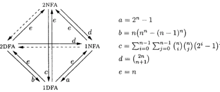
2. MOTIVATION 2NFA ea= 2' - 1 e _e n -' d _{b = n(n" - (n - 1)n)} 2DFA - -- - -- --- - -- do 1NFA C = En 1 n n 2 -n ) e ed=(") c e= n b " a 1DFA

FIGURE 1. The 12 conversions defined by nondeterminism and bidirectionality in finite automata, and the known exact trade-offs.

automata in the family D := (Dn)n o are exactly the values of the trade-off, and therefore D is not of polynomial size. Moreover, for

Hf

the language recognized

by Nn and Dn, the family H := (HT)g>o is clearly in 2N (because of the linear-size family N := (Nn),>o) but not in 2D (since D is not of polynomial size). Overall, 2D 2N.

Note the sharp difference in our understanding of the two conversions mentioned so far. On the one hand, our understanding of the conversion from 1NFAs to 1DFAs is perfect: we know the exact value of the associated trade-off. On the other hand, our understanding of the conversion from 2NFAs to 2DFAs is minimal: not only do we not know the exact value of the associated trade-off, but we cannot even tell whether it is polynomial or not. The best known upper bound for it is exponential, while the best known lower bound is quadratic. In fact, the details of this gap reveal a much more embarrassing ignorance. The exponential upper bound is the trade-off from 2NFAs to 1DFAs, while the quadratic lower bound is the trade-off from unary 1NFAs to 2DFAs. In other words, put in the shoes of a 2DFA that tries to simulate a 2NFA, we have no idea how to benefit from our bidirectionality; at the same time, put in the shoes of a 2NFA that tries to resist being simulated by a 2DFA, we have no idea how to use our bidirectionality or our ability to distinguish between different tape symbols.

A bigger picture is even more peculiar. The 12 arrows in Figure 1 show all possible conversions that can be performed between the four most fundamental types of finite automata: 1DFAs, 1NFAs, 2DFAs, and 2NFAs. For 10 of these conver-sions, the problem of finding the exact value of the associated trade-off has been completely resolved (as shown in the figure), and therefore our understanding of them is perfect. The only two that remain unresolved are the ones from 2NFAs and 1NFAs to 2DFAs (as shown by the dashed arrows), that is, exactly the conversions associated with 2D vs. 2N.

In conclusion, from the descriptional complexity perspective, the 2D vs. 2N problem represents the last two open questions about the relative succinctness of the basic types of automata defined by nondeterminism and bidirectionality. Moreover, the contrast in our understanding between these two questions and the remaining ten is the sharp contrast between minimal and perfect understanding.

(16)

INTRODUCTION

3. Progress

Our progress against the 2DVS. 2N question has been in two distinct directions: we have proved lower bounds for automata of restricted information and for au-tomata of restricted bidirectionality. In both cases, our theorems involve a particular computational problem called liveness. We start by describing this problem.

3.1. Liveness. As already mentioned in Section 2.1-III, we currently believe

that 2NFAs can be exponentially smaller than 2DFAs even without using their bidi-rectionality. That is, we believe that even INFAs can be exponentially smaller than 2DFAs. In computational complexity terms, this is the same as saying that the reason why 2D 2N is because already 2D IN, where iN is the class of fami-lies of regular problems that can be solved by polynomial-size famifami-lies of 1NFAs. In descriptional complexity terms, this is the same as saying that the reason why the trade-off from 2NFAs to 2DFAs is not polynomially bounded is because already the trade-off from 1NFAs to 2DFAs is not. In this thesis, we focus on this stronger conjecture.

As in any attempt to show non-containment of one complexity class into another (P 0 NP, L 0 NL), it is important to know specific complete problems-namely, problems which witness the non-containment iff the non-containment indeed holds. In our case, we need a family of regular problems that can be solved by a polynomial-size family of 1NFAs and, in addition, they are such that no polynomial-size family of 2DFAs can solve them iff 2D i IN. Such families are known. In fact, we have already presented one: the family of problems defined on page 8 over the alphabets An. So, it is safe to invest all our efforts in trying to understand that particular family, and prove or disprove the 2D i IN conjecture by showing that the family does not or does belong to 2D. However, it is easier (and as safe) to work with another complete family, which is defined over an even larger alphabet and thus brings us closer to the combinatorial core of the conjecture. This family is called

liveness, denoted by B = (Bn)n>o, and defined as follows [48].

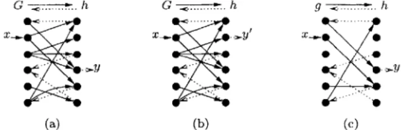
For each n, we consider the alphabet En := P({1, 2, ... , n}2) of all directed

2-column graphs with n nodes per 2-column and only rightward arrows. For example, for n = 5 this alphabet includes the symbols:

where, e.g., indexing the vertices from top to bottom, the rightmost symbol is {(1, 2), (2,1), (4, 4), (5, 5)}. Given an m-long string over En, we naturally interpret it as the representation of a directed (m + 1)-column graph, the one that we get by identifying the adjacent columns of neighboring symbols. For example, for m 8 the string of the above symbols represents the graph:

0 1 2 3 4 5 6 7 8

4 .---. *

where columns are indexed from left to right starting from 0. In this graph, a

live path is any path that connects the leftmost column to the rightmost one (i.e.,

the Oth to the mth column), and a live vertex is any vertex that has a path from 16

(17)

3. PROGRESS

the leftmost column to it. The string is live if live paths exist; equivalently, if the rightmost column contains live vertices. Otherwise, the string is dead. For example, in the above string, the 5th node of the 2nd column is live because of the

path 3 -+ 3 -+ 5, and the string is live because of two live paths, one of which is 3 -+ 3 -+ 2 -+ 5 -> 5 -* 3 --+ 3 --> 2 -+ 1. Note that no information is lost if we

drop the direction of the arrows, and we do. So, the above string is simply:

The problem B, consists in determining whether a given string over

**E*,**

is live or not. In formal dialect, we define B, := {w E Z* I w is live }, for all n.

As already claimed, B c IN. That is, there exist small 1NFA algorithms for B,. The smallest possible one is rather obvious:

We scan the list of graphs from left to right, trying to nondetermin-istically follow one live path. Initially, we guess the starting vertex among those of the leftmost column. Then, on reading each graph, we find which vertices in the next column are accessible from the most recent vertex. If none is, we hang (in this branch of the nondeter-minism). Otherwise, we guess one of them and move on remembering only it. If we ever arrive at the end of the input, we accept.

It is easy to verify that this algorithm can be implemented on a 1NFA with exactly one state per possible vertex in a column. Hence, B, is solvable by an n-state 1NFA.

In contrast, nobody knows how to solve B, on a 2DFA with fewer than 2' -1 states. The best known 2DFA algorithm is the following:

We scan the list of graphs from left to right, remembering only the set of live vertices in the most recent column. Initially, all vertices of the leftmost column are live. Then, on reading each graph, we use its arrows to compute the set of live vertices in the next column. If it is empty, we simply hang. Otherwise, we move on, remembering only this set. If we ever arrive at the end of the input, we accept.

Easily, this algorithm needs exactly one state per possible non-empty set of live vertices in a column, for a total of 2' - 1 states, as promised.

By the completeness of B, our questions about the relation between 2D and IN can be encoded into questions about the size of a 2DFA solving B". In other words, the following three statements are equivalent:

" 2D D 1N,

" the trade-off from 1NFAs to 2DFAs is polynomially bounded,

" B, can be solved by a 2DFA of size polynomial in n.

Hence, to prove the conjecture that 2D iN, we just need to prove that the number of states in every 2DFA solving B, is super-polynomial in n. In fact, as explained in Section 2.1-III, a stronger conjecture says that the above 2DFA algorithm is optimal! That is, in every 2DFA solving Ba-the conjecture goes-the number of states is not only super-polynomial but already 2' -1 or bigger. To better understand what this means, observe that the above algorithm is one-way: it is, in fact, the smallest

1DFA for liveness (as we can easily prove). Therefore, the claim is that in solving

liveness, a 2DFA has no way of using its bidirectionality to save even 1 of the 2n - 1

states that are necessary without it.

(18)

INTRODUCTION

3.2. Restricted information: Moles. The first direction that we explore in our investigation of the efficiency of 2DFAs against liveness is motivated by the particular way of operation of the 1NFA algorithm that we described above.

Specifically, consider any branch of the nondeterministic computation of that

1NFA. _{Along that branch, the automaton moves through the input from left to right,}

reading one graph after the other. However, although at every step the entire next graph is read, only part of its information is used. In particular, the automaton 'focuses' only on one of the vertices in the left column of the graph and 'sees' only the arrows which depart from that vertex. The rest of the graph is ignored. In this sense, the automaton operates in a mode of 'restricted information'.

A more intuitive way to describe this mode of operation is to view the input string as a 'network of tunnels' and the

1NFA

as an n-state one-way nondeterministic robot that explores this network. Then, at each step, the robot reads only the index of the vertex that it is currently on and the tunnels that depart from that vertex, and has the option to either follow one of these tunnels or abort, if none exists. In yet more intuitive terms, the automaton behaves like an n-state one-way nondeterministic mole.

Given this observation, a natural question to ask is the following: Suppose we apply to this mole the same conversion that defines the question whether 2D D IN. Namely, suppose that this mole loses its nondeterminism in exchange for bidirec-tionality. How much larger does it need to get to still be solving B"? That is, can

liveness be solved by a small two-way deterministic mole? Equivalently, is there

a 2DFA algorithm that can tell whether a string is live or not by simply exploring the graph defined by it? Note that, at first glance, there is nothing to exclude the possibility of some clever graph exploration technique that correctly detects the existence of live paths and can indeed be implemented on a small 2DFA.

In Chapter 2 we prove that the answer to this question is strongly negative:

no two-way deterministic mole can solve liveness.

To understand the value of this answer, it is necessary to understand both the "good news" and the "bad news" that it contains.

The good news is that we have crossed an entire, very natural class of 2DFA algorithms off the list of candidates against liveness. We have thus come to know that every correct 2DFA must be using the information of every symbol in a more complex way than moles.

However, note that our answer talks of all two-way deterministic moles, as opposed to only small ones. This might sound like "even better news", but it is actually bad. Remember that our primary interest is not moles themselves, but rather the behavior of small 2DFAs against liveness. So, our hope was that we would get an answer that involves small moles, and this hope did not material-ize. Put another way, we asked a complexity-theoretic question and we received a computability-theoretic answer.

Overall, our understanding has indeed advanced, but not for the class of ma-chines that we were mostly interested in. Nevertheless, some of the tools developed for the proof of this theorem may still be useful for the more general goal. Specifi-cally, if indeed small 2DFAs cannot solve liveness, then it is hard to imagine a proof that will not involve very long inputs. Such a proof will probably need tools similar to the dilemmas and generic strings for 2DFAs that were used in our argument.

(19)

3. PROGRESS

3.3. Restricted bidirectionality: Sweeping automata. The second direc-tion that we explore is motivated by the known fact that 2D is closed under com-plement [54, 14], whereas the corresponding question for 2N is open. So, one way to prove that 2D / 2N is to show that 2N is not closed under complement. In terms of classes, we can write this goal as 2N 4 co2N, where co2N is the class of families of regular problems whose complements can be solved by polynomial-size families of 2NFAs. Of course, it is conceivable that 2N = co2N, in which case a proof of this would be evidence that 2D = 2N.

As a matter of fact, 2N = co2N is already known to hold in some special cases. First, the analogue of this question for logarithmic-space Turing machines is known to have been resolved this way: NL = coNL [24, 58]. By the argument of [3],

this implies that every small 2NFA can be converted into a small 2NFA that makes exactly the opposite decisions on all "short" inputs (in the sense of Section 2.1-IV). In addition, the proof idea of NL = coNL has been used to prove that indeed 2N = co2N for the case of unary regular problems [14]. So, 2N and co2N are already known to coincide on short and on unary inputs.

However, there is little doubt that the above special cases avoid the core of the hardness of the 2N vs. co2N question. In this sense, our confidence in the conjecture that 2N = co2N is not seriously harmed. As a matter of fact, in Chapter 2 we prove a theorem that constitutes evidence for it. We consider a restriction on the bidirectionality of the 2NFAs and prove that, under this restriction, 2N

#

co2N. The restricted automata that we consider are the "sweeping" 2NFAs.

A two-way automaton is called sweeping if its input head can change the direc-tion of its modirec-tion only on the two ends of the input. In other words, each computa-tion of a sweeping automaton is simply a sequence of one-way passes over the input, with alternating direction. We use the notation SNFA for sweeping 2NFAs, and SN for the class of families of regular problems that can be solved by polynomial-size families of SNFAs. With these names, our theorem says that:

SN 4 coSN.

More specifically, our proof uses liveness, which is obviously in SN: B E SN. We prove that, in contrast, every SNFA solving the complement of B" needs ₂0(n) states,

so that B V coSN. Overall, B E SN \ coSN and the two classes are different.

Another way to interpret this theorem is to view it as a generalization of two other, previously known facts about the complement of liveness: that it is not

solv-able by small INFAs [48] and that it is not solvable by small sweeping 2DFAs [55, 14],

either. So, proving the same for small SNFAs amounts to generalizing both these facts to sweeping bidirectionality and to nondeterminism, respectively. For another interesting interpretation, note that the smallest known SNFA solving the comple-ment of B, is still the obvious 2"-state 1DFA from page 17. Hence, our theorem says that, even after allowing sweeping bidirectionality and nondeterminism together, a 1DFA can still not achieve significant savings in size against the complement of liveness-whether it can save even 1 state is still open.

Finally, our proof can be modified so that all strings used in it are drawn from a special subclass of Z* on which the complement of liveness can actually be determined by a small 2DFA. This immediately implies that:

the trade-off from 2DFAs to SNFAs is exponential,

which generalizes a known similar relation between 2DFAs and SDFAs [55, 2, 36].

(20)

INTRODUCTION

4. Other Problems in This Thesis

Apart from the progress against the 2D vs. 2N question explained above, this thesis also contains a few other, related theorems in descriptional complexity.

4.1. Exact trade-offs for regular conversions. As explained in Section 2.2 (Figure 1), the 2D vs. 2N question concerns only 2 of the 12 possible conversions between the four most basic types of finite automata (1DFAs, 1NFAs, 2DFAs, and 2NFAs). For each of the remaining conversions our understanding is perfect, in the sense that we know the exact value of the associated trade-off.

For the conversion from 1NFAs to 1DFAs (Figure la), the upper bound is due to [47] and the lower bound due to [35]. For any of the conversions from weaker to stronger automata (Figure le), the upper bound is obvious by the definitions and the lower bound is due to [6]. For the remaining four conversions (from 2NFAs

or 2DFAs to 1NFAs or 1DFAs), both the upper and lower bounds are due to this thesis-although the fact that the trade-offs were exponential was known before. We establish these exact values in Chapter 1. For a quick look, see Figure lb-d.

We stress, however, that the exact values alone do to reveal the depth of the understanding behind the associated proofs. In order to explain what we mean by this, let us revisit the conversion from 1NFAs to 1DFAs. As already mentioned, we can encode our understanding of this conversion into the concise statement that:

the trade-off from 1NFAs to 1DFAs is exactly 2' - 1. A less succinct but more informative description is that, for all n:

" every n-state 1NFA has an equivalent 1DFA with at most 2' - 1 states, and " some n-state 1NFA has no equivalent 1DFA with fewer than 2' - 1 states. But even these more verbose statements fail to describe the kind of understanding that led to them. What we really know is that every 1NFA N can be simulated by

a 1DFA that has 1 distinct state for each non-empty subset of states of N which (as an instantaneous description of N) is both realizable and non-redundant. This is exactly the idea where everything else comes from: the value 2n - 1 (by a standard counting argument), the simulation for the upper bound (just construct a 1DFA with these states and with the then obvious transitions), and the hard instances for the lower bound (just find INFAs that manage to keep all of their instantaneous descriptions realizable and non-redundant). In this sense, we know more than just the value of the trade-off; we know the precise, single reason behind it:

the non-empty subsets of states of the 1NFA

that is being converted. To be able to pin down the exact source of the difficulty of a conversion in terms of such a simple and well-understood class of set-theoretic objects is a rather elegant achievement.

Our analyses in Chapter 1 are supported by this same kind of understanding: in each one of the four trade-offs that we discuss, we first identify the correct set-theoretic object at the core of the conversion and then move on to extract from it the exact value, the simulation, and the hard instances that we need. As a foretaste, here are the objects at the core of the conversion from 2NFAs to 1NFAs:

the pairs of subsets of states of the 2NFA being converted, where the second subset has exactly 1 more state than the first subset.

So, every 2NFA can be simulated by a 1NFA that has 1 distinct state for every such pair, and for some 2NFAs all these states are necessary. Moreover, the value of the

(21)

4. OTHER PROBLEMS IN THIS THESIS

trade-off is exactly the number of such pairs that we can construct out of an n-state 2NFA; a standard counting argument shows that this number is

(n1).

4.2. Non-recursive trade-offs for non-regular conversions. In contrast to Chapters 1 and 2, the last chapter studies conversions between machines other than the automata of Figure 1, including machines that can also recognize non-regular problems. As we shall see, the trade-offs for such conversions may, in general, behave in a quite different manner.

To understand the difference, note that already since [53] we knew how to effectively convert any 2NFA (the strongest type of automata in Figure 1) into a

1DFA (the weakest type). This immediately guaranteed a recursive upper bound for each one of the 12 trade-offs of Figure 1. In contrast, for other conversions, such a recursive upper bound cannot be taken for granted. As first shown in [35], there are cases where the trade-off of a conversion grows faster than any recursive function: e.g., the conversion from one-way nondeterministic pushdown automata that recognize regular languages to 1DFAs. Moreover, this phenomenon cannot be attributed simply to the difference in power between the types of the machines involved. As shown in [56], if the pushdown automata in the previous conversion are deterministic, then the trade-off does admit a recursive upper bound. Such trade-offs, that cannot be recursively bounded, are simply called non-recursive. Note that this name is slightly misleading, as it allows the possibility of a non-recursive trade-off that still admits non-recursive upper bounds. However, no such cases will appear in this thesis.

In Chapter 3 we refine a well-known technique [16] to prove a general theorem that implies the non-recursiveness of the trade-off for a list of conversions involving two-way machines. Roughly speaking, our theorem concerns any two types of machines, A and B, that satisfy the following two conditions:

" the A machines can solve problems that no B machine can solve, and

" the A machines can simulate any two-way deterministic finite automaton that

works on a unary alphabet and has access to a linearly-bounded counter.

For any such pair of types, our theorem says that the trade-off from A machines to B machines is non-recursive. For example, we can have A be the multi-head finite

automata with k + 1 heads and B be the multi-head finite automata with k heads.

No matter what k is, the conditions are known to be true, and therefore replacing a multi-head finite automaton with an equivalent one that has 1 fewer head results in an non-recursive increase in the size of the automaton's description, in general.

At the core of the argument of this theorem lies a lemma of independent interest: we prove that the emptiness problem remains unrecognizable (non-semidecidable) even for a unary two-way deterministic finite automaton that has access to a linearly-bounded counter and obeys a threshold-in the sense that it either rejects all its inputs or accepts exactly those that are longer than some fixed length.

(22)

(23)

CHAPTER 1

Exact Trade-Offs

In this chapter we prove the exact values of the trade-offs for the conversions from two-way to one-way finite automata, as pictured in Figure 1 (page 15). In Section 3 we cover the conversion from 2DFAs to 1DFAs (Figure

1b),

whereas the conversion from 2NFAs to 1DFAs (Figure 1c) is the subject of Section 4. The

conver-sions from 2NFAs and 2DFAs to 1NFAs (Figure 1d) are covered together in Section 5.

We begin with a short note on the history of the subject and a summary of our conclusions.

1. History of the Conversions

The conversion from INFAs to 1DFAs is the archetypal problem of descriptional complexity. As already mentioned (Figure

la),

the problem is fully resolved, in the sense that we know the exact value of the associated trade-off:1

the trade-off from 1NFAs to 1DFAs is 2n - 1.

The history of this problem began in the late 50's, when Rabin and Scott [46, 47] introduced INFAs as a generalization of

1DFAs

and showed how

1DFAs

can simulate them. This proved the upper bound for the trade-off. The matching lower bound was established much later, via several examples of "hard"

1NFAs

[44, 35, 43, 51, 48, 33].2 Both bounds are based on the crucial idea that

the non-empty subsets of states of the

1NFA

capture everything that a simulating

1DFA

needs to describe with its states. As part of the same seminal work [45, 47], Rabin and Scott also introduced

two-way automata and proved "to their surprise" that 1DFAs were again able to sim-ulate their generalization. This time, though, the proof was complicated enough to be superseded by a simpler proof by Shepherdson [53] at around the same time. All authors were actually talking about what we would now call single-pass two-way

de-terministic finite automata (ZDFAs), as their definitions did not involve end-markers. However, the automata quickly grew into full-fledged two-way deterministic finite

automata (2DFAs) and also into nondeterministic counterparts (ZNFAs and 2NFAs),

while all theorems remained valid or easily adjustable.

Naturally, the descriptive complexity questions arose again. Shepherdson men-tioned that, according to his proof, every n-state 2DFA had an equivalent 1DFA with at most (n+ 1)(n+1) states. Had he cared for his bound to be tight, he would surely

1

Recall our conventions, as explained in Footnote 2 on page 12. 2

The earliest ones, both over a binary alphabet, appeared in (35] (an example that was described as a simplification of one contained in an even earlier unpublished report [44]) and in [43] (where [44] is again mentioned as containing a different example with similar properties). Other examples have also appeared, over both large [51, 48] and binary alphabets [33]. A more natural but not optimal example was also mentioned in [35] and attributed to Paterson.