2004 by the Genetics Society of America DOI: 10.1534/genetics.104.028993
Quantitative Trait Loci (QTL) Detection in Multicross Inbred
Designs: Recovering QTL Identical-by-Descent Status
Information From Marker Data
Se´bastien Crepieux,*
,1Claude Lebreton,
†Bertrand Servin
‡and Gilles Charmet*
*UMR 1095 INRA-UBP, 63039 Clermont-Ferrand Cedex 2, France,†Limagrain Verneuil Holding, site d’ULICE, F-63204 RiomCedex, France and‡INRA UMR de Ge´ne´tique Ve´ge´tale, INRA/UPS/INAPG, 91 190 Gif sur Yvette, France
Manuscript received March 18, 2004 Accepted for publication August 10, 2004
ABSTRACT
Mapping quantitative trait loci in plants is usually conducted using a population derived from a cross between two inbred lines. The power of such QTL detection and the parameter estimates depend largely on the choice of the two parental lines. Thus, the QTL detected in such populations represent only a small part of the genetic architecture of the trait. In addition, the effects of only two alleles are characterized, which is of limited interest to the breeder, while common pedigree breeding material remains unexploited for QTL mapping. In this study, we extend QTL mapping methodology to a generalized framework, based on a two-step IBD variance component approach, applicable to any type of breeding population obtained from inbred parents. We then investigate with simulated data mimicking conventional breeding programs the influence of different estimates of the IBD values on the power of QTL detection. The proposed method would provide an alternative to the development of specifically designed recombinant populations, by utilizing the genetic variation actually managed by plant breeders. The use of these detected QTL in assisting breeding would thus be facilitated.
T
HE availability of molecular markers in the 1980s called the fixed-model approach (Xu and Atchley 1995) since it considers a fixed number of distinct alleles opened a new scope for quantitative genetics andbreeding. It was anticipated that the manipulation of (most often two) at each putative QTL. Statistical meth-ods for the QTL analysis of biparental populations un-loci underlying quantitative traits (QTL) would be as
easily feasible as with Mendelian factors. This, however, derwent successive improvements through the advent of interval mapping (Lander and Botstein 1989) and has generally not been the case, despite the large corpus
of theoretical studies on marker-assisted selection (MAS; its linearization (Haley and Knott 1992), composite interval mapping (Zeng 1993, 1994; Jansen 1993), and
e.g., Lande and Thompson 1990; Gimelfarb and Lande
1994, 1995; Hospital et al. 1997). The main reason multiple-trait QTL mapping ( Jiang and Zeng 1995; Korol et al. 1995).
is probably the cost of markers and the relatively low
In contrast, breeder’s material is distinct from the improvement in selection efficiency that leads MAS to
biparental populations studied in many mapping exper-be generally much more expensive than conventional
iments. Breeders generally handle many small-sized fam-breeding (Moreau et al. 2000). The other reason is that
ilies derived from crosses between (often highly related) applied breeding programs and QTL research are often
elite lines. The methods described above are poorly disconnected, i.e., performed by different teams and
suited to such material. Moreover, there are many draw-using different plant material.
backs for the breeder’s use of the QTL found on bipa-Generally, QTL analyses are carried out on a few
rental populations. First, when only two parents are progenies from crosses between a small number of
dis-considered, some markers and potential QTL are more tantly related lines, often including wild relatives. Such
likely to be monomorphic, even if parental lines are analyses mostly involve biparental progenies such as
carefully selected for trait divergence. Since, by defini-backcrosses (BC), doubled haploid lines (DH), F2, or
tion, QTL can be found only at polymorphic sites in recombinant inbred lines (RILs). In the approaches
the genome, the expected number of QTL detected based on this kind of plant material, the effect of an
with a biparental cross will be lower than that expected allele substitution at a candidate locus is tested. This is
when analyzing several crosses at a time (assuming the total number of genotypes is not the limiting factor). The second drawback is that the QTL effect is estimated
1Corresponding author: Limagrain Verneuil Holding, site d’ULICE,
as a contrast between two alleles and in one genetic
av. G. Gershwin, BP173, F-63204 Riom Cedex, France.
E-mail: [email protected] background only. In that context, the improvement of Genetics 168: 1737–1749 (November 2004)
a line by the introgression of a QTL allele into a com- tation of the IBD matrices (see George et al. 2000 for a review). The IBD status between two individuals can pletely new genetic background is rather unpredictable,
be precisely inferred if the relationship between the two because of possible epistatic interaction between QTL
individuals (i.e., the pedigree) is known and if ancestors and genetic background. Finally, from an economic
in the pedigree can be genotyped. Most of the existing standpoint, the cost of creation of large single-cross
methods to compute IBD probabilities [see, for instance, progenies and specific trials for trait evaluation to
per-the software LOKI (Heath 1997), SOLAR (Almasy and form QTL detection is quite high and often at the
ex-Blangero 1998), and SIMWALK2 (Sobel et al. 2001)] pense of other selection programs.
were developed for human and animal genetics and are All these drawbacks reduce the breeder’s interest in
not directly applicable to the particularities of plants implementing such experimental designs when funding
(inbreeding, self-pollination, controlled mating, selec-and work are constrained. Biparental crosses are usually
tion . . .). Moreover, in such methods, if unknown rela-preferred for more upstream studies, e.g., genomics: the
tionships exist between parents of individuals of the fine mapping of a QTL, which is a prerequisite for
mapping population, then parents are considered as its positional cloning, is easier when fewer QTL are
founders. This statement yields systematically for non-segregating. In contrast, the breeder’s focus will be to
sibs IBD likelihood of zero at any position on their characterize the effect of a wide range of alleles in his
genome, even if it is commonly assumed in plant breed-germplasm. Methods for simultaneous detection and
ing programs that most of the parents share common manipulation of QTL in breeding programs would thus
“unknown” ancestors (use of some “star” varieties; see enhance the applicability of MAS.
Bernardo 1993, for example). Furthermore, in frag-Muranty (1996) suggested the use of progenies from
mented situations, i.e., where there are many families several parents, to achieve a high probability of obtaining
of small sizes (especially when the genotyping takes more than one allele at a putative QTL and also to have
place at a late stage in pedigree breeding, where we a more representative estimate of the variance accounted
may easily end up with as few as one or two lines per for by a QTL. Xu (1998) compared the QTL detection
cross), the IBD-likelihood matrix can be very sparse. powers obtained with random-effect models and fixed
Hence, much could be gained in exploring the actual effects and found similar values for individual family
between-family IBD likelihoods in cases where only little sizes as low as 25 individuals. However, in more
unbal-information is available. anced designs, the random-effect approach was
pre-In this article, we continued these developments and sumed to be more suited as it can handle any arbitrary
further assumed a nonzero IBD likelihood between non-pedigree of individuals (Lynch and Walsh 1998; Xu
sib lines. For that, we devised a method to take into 1998). Efficient methodologies for more fragmented
account an estimate of the coefficients of coancestries populations in plants have been developed (for
exam-between parents to build the IBD matrices and present ple, Xie et al. 1998; Yi and Xu 2001; Bink et al. 2002;
a unified IBD-based variance component analysis frame-Jansen et al. 2003), but their extension or
implementa-work, to map QTL in any kind of multicross designs tion for any complex plant designs, implying a mixture
involving self-pollinating species, at any generation. of half-sib and full-sib families of different sizes, at any
To test the accuracy of the method, we considered generation of selfing, is not straightforward. The identi- the most general case of pedigree breeding programs, cal-by-descent (IBD)-based variance component analysis where many different two-parent crosses are performed, is a powerful statistical method for QTL mapping in each yielding very small progenies in advanced genera-complex populations and can be used in pedigrees of tions of selfing. We then investigated the influence of arbitrary size and complexity (Almasy and Blangero different methods of IBD computation on the power 1998). These IBD-based variance component analyses and accuracy to detect QTL on different complex popu-are derived from the assumption that individuals of lations similar to those used in breeding.
similar phenotype are more likely to share alleles that are identical by descent. The construction of IBD
matri-METHODS ces for alleles at each position tested along the genome
and the fitting of random-effect models (which assumes Plant breeding material—multicross inbred designs: that QTL effects are normally distributed) offer an ap- In this article, we consider a mapping population com-propriate method to map QTL if the mapping popula- posed of several subpopulations of small size. Each of tion is large enough and if the progenies are connected these subpopulations is composed of as few as one off-in some way. In addition, these models do not need to spring coming from a single cross between two inbred assume a known, finite set of alleles at each putative parents. For example, these subpopulations could be QTL. Thus, they offer a less parameterized statistical produced by several consecutive selfings (e.g., RILs) or environment in which to map QTL, because only the backcrossings. We use the terms “parent,” “half-sib,” and variances need to be estimated instead of every allele “full-sib” in a broadened sense. By parents, we mean substitution effect. IBD-based variance component ap- the two inbred lines that are crossed with each other to start a new breeding cycle. By full-sib, we mean indi-proaches mostly differ from one another in the
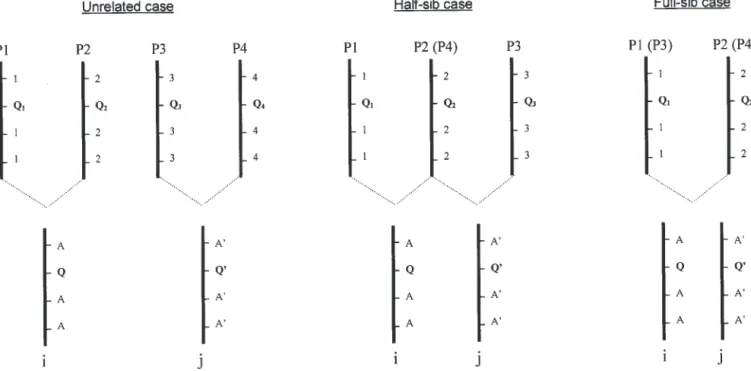
compu-viduals derived from the same initial cross (i.e., involving First, we draw relevant calculations of the IBD values for each of these cases (Figure 1).
the same two parents), after any number of selfing and/
Computation of G matrices with parents considered
or backcrossing generations. By half-sib, we mean
indi-as founders: Exact IBD value between two individuals at a
viduals sharing one parent in common, after any
num-QTL: Within each subpopulation, only two alleles are
ber of selfing and/or backcrossing generations. Any
segregating at each locus, giving only three possible individuals that do not share any parent in common
genotypes at the QTL, for example, Q1Q1, Q1Q2, and
are termed “unrelated.” The definitions are more
rele-Q2Q2.
vant to plants, since our phenotyped progenies may
Suppose that one of the subpopulations is composed commonly be as far as six or seven generations from
of two individuals (i and j ) that are thus full-sibs. The their parents. Nevertheless, in a general case, the
ge-IBD value between two full-sibs i and j at a QTL is mea-nome of the individuals of the mapping population
sured as could be fixed (i.e., lines), fully heterozygous (i.e., F1),
or a mixing of fixed and heterozygous parts (i.e., issued
i,j⫽ 2i,j
from successive backcrossing or selfing generations).
Mixed linear models:We assume that the quantitative
⫽
冦
2 for Q1Q1⫺ Q1Q1or Q2Q2⫺ Q2Q2
1 for Q1Q1⫺ Q1Q2, Q2Q2,⫺ Q1Q2, or Q1Q2⫺ Q1Q2
0 for Q1Q1⫺ Q2Q2,
trait value is a linear combination of fixed design effects, putative QTL (with additive or/and dominance effects), and additive polygenic effects. The polygenic effect is
i,jbeing the IBD value between individuals i and j, at
seen as the cumulative effect of all loci affecting the a putative QTL (
i,j represent also the ijth elements
quantitative trait that are unlinked to the QTL. The of G), and
i,jbeing Malecot’s (1948) coefficient of
model without dominance effect is coancestry. If i and j are inbred,
ij is interpreted as
twice the coefficient of coancestry for the QTL (see Xie
y⫽ X ⫹ Zu ⫹ Zv ⫹ e, (1)
et al. 1998 for the interpretation of the inbred case).
In the same manner, the IBD values between two half-where y is an (m ⫻ 1) vector of phenotypes, X is an
sibs i and j at a QTL are measured as (m ⫻ s) design matrix,  is a (s ⫻ 1) vector of fixed
effects, Z is an (m⫻ q) incidence matrix relating records
to individuals, u is a (q ⫻ 1) vector of additive QTL
i,j⫽ 2i,j⫽
冦
2 for Q2Q2⫺ Q2Q2
1 for Q1Q2⫺ Q2Q3
0 otherwise. effects, v is a (q⫻ 1) vector of additive polygenic effects,
and e is the residual vector. We assume the random
effects u, v, and e as uncorrelated and distributed as Finally, if individuals i and j are non-sibs, and their multivariate normal densities, parents are still supposed unrelated, they will share IBD
probability of 0.
uⵑ (0, G2
u), vⵑ (0, A2v), eⵑ (0, I2e), Inferring the IBD likelihood at a QTL from marker data:
The IBD value is determined by the genotypes of two with2
u,2v, and2ebeing, respectively, the additive
vari-individuals at the QTL of interest. The actual QTL geno-ance of the QTL, the polygenic varigeno-ance, and the
resid-type of an individual, however, is in most cases not ual variance. A is the (q⫻ q) additive genetic
relation-observable and must be inferred from flanking marker ship matrix; G is the (q⫻ q) (co)variance matrix for
information (that we term IM—this is represented in
the QTL additive effects conditional on marker
informa-Figure 1 by A and A⬘). tion; and I is the identity matrix.
We denote the following probabilities, suited for all The model without QTL segregating in the
popula-cases (full-sib and half-sib popula-cases are particularities of the tion is, with the same notations,
unrelated case), pi 2⫽ Pr(Q1Q1| IM), pi1⫽ Pr(Q1Q2| IM), pi 0 ⫽ Pr(Q2Q2|IM) and pj 2 ⫽ Pr(Q3Q3|IM), pj 1 ⫽ Pr(Q3
y⫽ X ⫹ Zv ⫹ e. (2)
Q4|IM), and pj 0⫽ Pr(Q4Q4|IM). It should be noted that
Computation and implementation of G and A matri- for half-sibs Q4 is replaced by Q2and for full-sibs Q3is
ces:To solve the mixed-linear model, we need to know replaced by Q1and Q4by Q2. We write pi⫽ [pi 2pi 1pi 0]T
Aand G matrices (y, X, Z, and I are known) to estimate and pj⫽ [pj 2pj 1pj 0]T.
2
u,2v, ande2. Starting from Xie et al.’s (1998) notations addressing
With the above definitions of the material, if we con- the case of full-sib individuals only, the conditional ex-pectations of the IBD values areˆi,j ⫽ E(i,j|IM)⫽ pTiCpj
sider a pair of individuals from the mapping population,
for between individuals andˆi,i⫽ E(i,i| IM)⫽ cTpi for
they may be (i) taken from the same subpopulation, in
the individual with itself, where which case they are full-sibs, or (ii) taken from two
different subpopulations. In this last case, if one of the parents is common to the two subpopulations, the two
C ⫽
冤
2 1 0 1 1 1 0 1 2冥
and c⫽冤
2 1 2冥
. individuals will be half-sibs; if the parents of the twosubpopulations are distinct, the two individuals are
Figure 1.—If parents (P1, P2, P3, and P4) are considered as founders, only three types of relationships exist between individuals i and j of the mapping population. Notations Q1, Q2, Q3, and Q4represent parents’ QTL information while Q and Q⬘ (unknown)
represent progenies’ i and j QTL information. In the same manner, 1, 2, 3, and 4 represent parents’ marker alleles information while A and A⬘ (supposedly known) represent progenies’ i and j marker information. Q1, Q2, Q3, and Q4are homozygous while
Q and Q⬘ can be heterozygous. The possible genotypes at the QTL for the three cases are as follows:
full-sib and half-sib case by introducing the coancestries parents. For the following, we still consider that the parents of the latest breeding cycle and the current between parents P1-P3 and P2-P4, denoted byP1P3and
P2P4. If parents are considered as founders, these coan- F(n )-derived lines are the only genotyped material.
However, we consider this time that the parents of the cestries can take only values 1 or 0. Thus, the new C
matrix can then be rewritten as C1: mapping population could come from previous
genera-tions of breeding. They are thus very likely to share common ancestors (due to the intensive use of some star
C1⫽
冤
2P1P3 P1P3 0
P1P3 1⁄2(P1P3⫹ P2P4) P2P4
0 P2P4 2P2P4
冥
. varieties, for instance), even if those ancestors cannot be genotyped. Thus, for the full-sib case example, we could take into account the probability that the two parents Note that for the full-sib case P1⫽ P3 and P2 ⫽ P4,
share IBD QTL alleles. For the unrelated case, we could so thatP1P3andP2P4are equal to one and the C1matrix
take into account the probability that P1-P3, P1-P4, P2-is similar to C. Similarly, the relevant C matrices for
P3, or P2-P4 share IBD QTL so that Q1⬅ Q3, Q1⬅ Q4,
half-sib individuals can be obtained by replacing P1P3
Q2⬅ Q3, and Q2⬅ Q4. If we are able to estimate these
by zero and P2P4 by one—or P1P3 by one and P2P4 by
probabilities, they could be used to improve the compu-zero (and, for unrelated individuals, by replacing both
tation ofˆi,j’s. For the following, we supposed that
esti-P1P3andP2P4by zero).
mates of these probabilities between all parents were This formula, using the C1matrix (with the’s being
available. We take the more general case, i.e., the unre-equal to 0 or 1 only) for computing the IBD values, is
lated one, to draw a general formula that incorporates referred to as formula 1 in the rest of the article.
these estimates and that covers the three cases of
rela-Computation of G matrices with parents not
consid-tionships between individuals of the mapping
popula-ered as founders:Using the above formula to compute
tion. We denote byP1P3,P1P4,P2P3, andP2P4the estimates
ˆi,j’s, we assumed that parents of subpopulations were
of the coefficients of coancestries between the four par-unrelated; i.e., they did not share any common
ances-ents. tors. Thus, to infer the IBD probabilities in the previous
First, we generalized above the C matrix to the known case, we did not need to have more genotypic
coan-cestries between parents P1-P3 and P2-P4, giving the C1 2 ⫻ 0.125. Thus, this information would be used in
formula 2 to improve the accuracy of the IBD estimate. matrix.
Similarly, taking into account the coefficients be- The second way to estimate these coefficients is to use the available molecular marker information. Nei tween the parents P1 and P4 on one hand and P2 and
P3 on the other hand, we can write the C2 matrix as and Li’s (1979) formula can be used to calculate the
genetic similarity index (GS): GS ⫽ 2Nij/(Ni ⫹ Nj),
where Nijis the number of alleles in common between
C2⫽
冤
0 P2P3 2P2P3
P1P4 1⁄2(P2P3⫹ P1P4) P2P3
2P1P4 P1P4 0
冥
. genotypes i and j, and N
i and Nj are the total number
of alleles observed for genotypes i and j, respectively.
Implementation of the IBD formula: We used the
Finally, with these two matrices, we can draw a general
deterministic approach of the MDM program (Servin formula for the conditional expectation of the IBD
val-et al. 2002) to compute all the piand pjprobabilities, at
ues between two individuals coming from four (distinct
any generation of selfing or backcrossing. IBD values or not) inbred parents:
were computed every 3 cM. Two flanking markers were ˆi,j⫽ E(i,j| IM)⫽ pTiC1pj⫹ piTC2pj⫽ pTi(C1⫹ C2) pj; used to infer the genotypes’ probabilities. In the
fre-quent case where the two parents shared the same
i.e.,
marker alleles at one or two loci flanking the putative ˆi,j⫽ E(i,j| IM)⫽ 2(P1P3[(pj 2⫹1⁄2pj 1)(pi 2⫹1⁄2pi1)] QTL position, the next closest markers to the interval
were used. It can easily be demonstrated that the IBD ⫹ P1P4[(pj 2⫹1⁄2pj 1)(pi 0⫹1⁄2pi1)]
values calculated at a putative QTL will be more precise ⫹ P2P3[(pj 0⫹1⁄2pj 1)(pi 2⫹1⁄2pi1)] if the flanking markers are highly polymorphic.
Solving of the mixed-linear models and test statistic
⫹ P2P4[(pj 0⫹1⁄2pj 1)(pi 0⫹1⁄2pi1)]).
under the null hypothesis: Two-step IBD-based variance
The conditional expectation of the IBD for an individual component method: The method used to map QTL in a
with itself remains complex inbred pedigree is then similar to all
interval-mapping-based variance component methods. It is com-ˆi,i⫽ E(i,i| IM)⫽ 2pi 2⫹ pi1⫹ 2pi 0.
posed of two steps (two-step IBD-based variance compo-nent method), as described in George et al. (2000). In In the rest of the article, this formula, using the C1and
C2 matrices to compute IBD values, is referred to as step 1, we computed the G matrices according to the
formula tested, for all the scanned positions. We then formula 2.
Please note that in the case of two full-sib individuals, inverted and wrote them in ASREML (Gilmour et al. 1998) format for user-defined inverse (co)variance ma-the probability that ma-the two parents P1 and P2 share
initially IBD QTL is taken into account in formula 2 by trices. We also computed the appropriate additive rela-tionship matrix A, inverted it, and wrote it in ASREML replacing P3 by P1 and P4 by P2 (P1 and P2 are
consid-ered as the parents of the first full-sib, P3 and P4 as the format. In step 2, ASREML provided restricted maxi-mum-likelihood (REML) estimates of steps 1 and 2. To parents of the second full-sib). Thus, both P1P3 and
P2P4will take values of one (accounting for the full-sib test for the presence of a QTL against no QTL at a
particular chromosomal position, we used the log-likeli-relationship with parents considered as founders—
similar to the formula of Xie et al. 1998) while bothP1P4 hood-ratio test: LR⫽ ⫺2 ln[L0(H0, no QTL present)⫺ L1 (H1, QTL present)], where L1and L0 represent the
andP2P3will be written asP1P2(accounting for possible
coancestry between parent P1 and P2). likelihood values of steps 1 and 2 evaluated at the REML solutions, respectively.
Estimates of the coefficients of coancestries: With
the above formula 2, it may be seen that accurate esti- Test statistic under the null hypothesis: The choice of a test statistic threshold is always challenging in this mates of the coefficients of coancestries between parents
of individuals i and j of the mapping population are kind of situation. As mentioned by George et al. (2000) permutation testing is problematic for such IBD-based needed for the computation of the G matrices (that are
built at each scanned position). These coefficients need variance component analysis since it is unclear how to permute the data while retaining the association be-also to be estimated between all the individuals i and j
of the mapping population, to account for polygenic tween polygenic variation and marker information. Many publications (Zeng 1994; Xu and Atchley 1995, variation through the relationship matrix A. There are
two main ways to estimate these coefficients of coances- for example) report that when a chromosomal interval is being scanned, the empirical distribution of LR fol-tries. The first one is to compute Malecot’s coefficients
on the basis of the available declared pedigrees and lows a mixture of two chi-square distributions, with 1 and 2 d.f., respectively. Since this article deals with simulated come back to the pedigree of each variety as far as
possible. For example, two parents of the mapping pop- data, it is possible to replicate data under the null hy-pothesis of no QTL segregating, construct the empirical ulation with a grandparent in common will share an
choosing the 95th percentile of the highest test statistic, elite, for example). Fourth, mass selection on the value of the quantitative trait was possible at each breeding generally over 500 or 1000 stochastic realizations. In
this article, we calculated an empirical threshold for cycle.
At every generation, a phenotype was simulated for each set of parameters, and then we ran 1000 additional
simulations with no QTL segregating on the scanned each individual line on the basis of its main QTL and polygene alleles. We performed QTL detection on the chromosome. We increased the polygenic variance such
that the total genetic variance remained unchanged and last breeding cycle.
Note that at the beginning of our breeding programs, determined the empirical threshold by choosing the
95th percentile from the list of 1000 runs. It should all the allele frequencies were equal, which was not the case after many generations due to genetic drift, be noted that this threshold is not genomewise but is
chromosomewise. nonpanmictic conditions, and selection. All the markers
and QTL were in full linkage disequilibrium at G0but
were not so after the breeding programs—the chromo-A SIMULchromo-ATION STUDY: THE Cchromo-ASE OF chromo-A PEDIGREE somes having undergone many recombinations. Hence,
BREEDING PROGRAM
as anticipated, a simple ANOVA was inefficient (results not shown).
We chose the case of pedigree breeding for the
simu-lation study as it contained most of the difficulties gener- Simulated populations: To illustrate the methodol-ogy, we focused only on two representative settings (two ally encountered in inbred breeding programs:
fre-quent lack of reliable pedigree information, beyond the complex populations of different size), for which we varied a limited number of parameters. For both set-parents (and thus unavailability of ancestor lines for
genotyping); possible genotyping only of advanced gen- tings, we initially fixed the following parameters: 20 founder lines (that initially correspond to 20 different erations of selfing, when the number of lines has
de-creased and the precision of trials inde-creased, constrain- alleles at each marker and QTL, with 20 different allele effects at the QTL), 21 chromosomes of length 100 ing the computation of IBD at the end of a breeding
cycle, without any marker information between the ini- cM each with 11 markers spaced every 10 cM, a QTL segregating at position 45 (half-way between two mark-tial cross and the resulting progenies (a breeding cycle
comprises the initial crosses between many different ers) on chromosome 1, and a total genetic heritability (QTL and polygenes) of 0.5. We fixed the number of parents to obtain the new improved lines after many
generations of self pollination); the very high number breeding cycles to 10 without selection and to 6 with selection (to retain genetic variance around the chro-of parents chro-of the mapping population yielding very small
full-sib families, and an uneven (L-shaped) distribution mosome 1 QTL and around the polygenes). The num-ber of polygenes varied from 40 for the cases without of half-sib family sizes; and the possible occurrence of
mass selection for the choice of the parents at the start selection to 9 and 4 with selection, for QTL heritabilities 0.05 and 0.1. We chose these numbers of polygenes in of a breeding cycle.
Simulation of the breeding program: An S-PLUS the case of selection to set an equivalent heritability for
each QTL and polygene to avoid the rapid fixation of (2000) function was developed to reproduce the typical
steps of pedigree-based plant breeding programs (see chromosome 1 QTL.
Setting 1 is composed of 300 inbred lines derived from
http://www.genetics.org/supplemental/ for a detailed
description). Briefly, we started by creating founder crosses between 50 parents chosen at random from the previous breeding cycles. Of 1225 different possible lines at the beginning of breeding (beginning of 20th
century, for instance). At this stage, the material was in crosses [(50⫻ 49)/2], 170 crosses per breeding cycle were simulated. Each cross gave, on average, 1.75 full-complete linkage disequilibrium, with as many alleles
as there were founder lines (for example, founder line sibs and each parent was found, on average, in 12 proge-nies. We simulated two groups of mapping populations: 1 carried only allele “1” for all the markers and QTL
. . .). In the first breeding cycle, we produced new germ- group a was obtained without the influence of selection on the quantitative trait, and group b was obtained plasm by crossing the founder lines together. Then,
during the following breeding cycles, we performed under the influence of selection on the quantitative trait for the choice of the parents at each generation.The crosses in a pedigree-breeding fashion. First a large
number of parents were used to obtain a reduced num- heritability of the chromosome 1 QTL was fixed for each population at 0.1.
ber of lines in advanced selfing generations (for
exam-ple, 100 parents are crossed to obtain only 500 individu- Setting 2 is composed of 500 individuals, derived from
crosses between 100 parents. Of 4950 different possible als at the end of a breeding cycle). Second, most of the
current parents were chosen among the lines derived crosses, 285 crosses per breeding cycle were simulated. Each cross gave, on average, 1.75 full-sibs and each par-from the most recent breeding cycles while a small part
was extracted from older breeding cycles (to represent ent was found, on average, in 10 progenies. We simu-lated different groups of populations, for different levels nonelite germplasm). Third, crosses were unevenly
TABLE 1
Main characteristics of the different mapping populations
Occurrence of selection No. of No. of marker
Mapping and simulated QTL and breeding No. of alleles flanking Effective no. of populations total genetic heritability cycles polygenes the QTL marker alleles Setting 1 (50 parents, 300 progenies) No, h2
QTL⫽ 0.1 10 40 10 5.5 h2 g⫽ 0.486 (0.083) Yes, h2 QTL⫽ 0.1 6 4 6 2.8 h2 g⫽ 0.478 (0.180)
Setting 2 (100 parents, 500 progenies) No, h2
QTL⫽ 0.05, 0.1, 0.2 10 40 14 6.2 h2 g⫽ 0.427, 0.435, 0.456 (ⵑ0.050) Yes, h2 QTL⫽ 0.05 6 9 13 4.5 h2 g⫽ 0.590 (0.210) Yes, h2 QTL⫽ 0.1 6 4 12 4 h2 g⫽ 0.550 (0.210)
The fixed parameters are 20 founder lines (i.e., initially 20 possible alleles at all the markers and QTL), 21 chromosomes of length 100 cM each with 11 markers spaced every 10 cM, and QTL segregating at position 45 on chromosome 1. The effective number of alleles is computed as Neff⫽ 1/兺N1f2, f being the allele frequencies and N the number of alleles. This effective
number of alleles is averaged at the two markers flanking the QTL (located on position 45 cM).
of selection: group a was obtained without the influence tween two individuals of the mapping population, and the A matrix will take the expected proportion of ge-of selection. We created the quantitative trait on the
mapping population (10th generation of breeding) for nome shared by two individuals, i.e., 2⫻ 0.5 if the two inbred individuals are full-sibs, 2⫻ 0.25 if the two inbred QTL heritabilities 0.05, 0.1, and 0.2. Group b was
ob-tained under the influence of selection on the value of individuals are half-sibs, 0 otherwise.
In setting 1, we used alternatively formulas 1, 2a, and the quantitative trait. We investigated two levels of QTL
heritability: 0.05 (with nine polygenes of 0.05 each) and 2b, while we used only formulas 1 and 2b in setting 2, due to computation time required for obtaining Malec-0.1 (with four polygenes of Malec-0.1 each).
Table 1 summarizes the main characteristics of the ot’s coefficients of coancestries for such important pop-ulations.
different mapping populations. It should be noted that
there were initially 20 alleles for each marker and QTL We tested every third centimorgan for the presence of a QTL. Under each condition, the detection was but that this number was greatly reduced after 6–10
breeding cycles, due to genetic drift and/or selection performed for 100 random replicates. Parameters esti-mates and their standard error are reported for all repli-pressure.
Methods compared: In this article, we investigated cates.
two different ways to infer the coefficients of coances-tries. We thus termed formulas 2a and 2b as follows:
RESULTS Formula 2a: Malecot’s coefficients of coancestries are
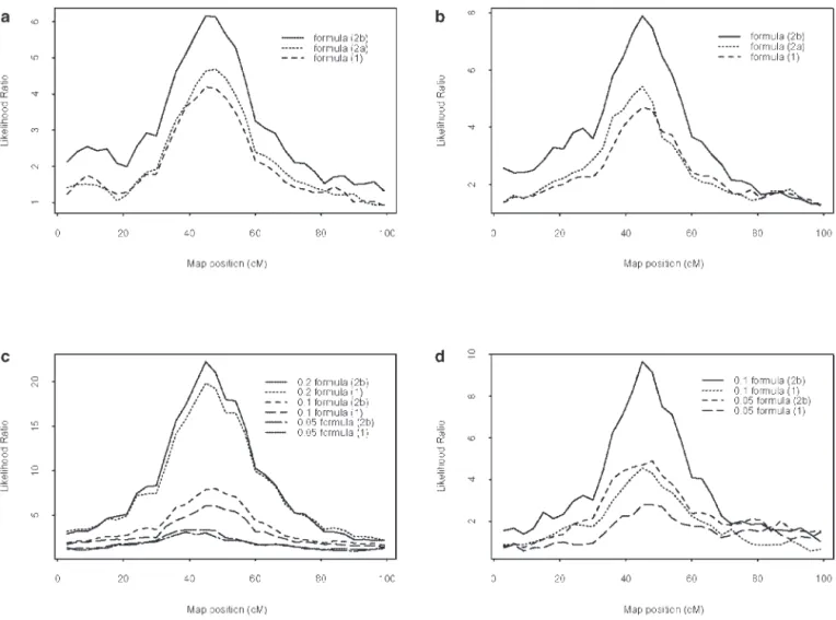
The average likelihood-ratio test profiles (over 100 used to build G (through formula 2) and A matrices.
replicates) are presented in Figure 2 for both settings. For that, full pedigree is stored during simulations
There was a strong influence of the formula on the LR and used to compute parents’ and progenies’
coeffi-profile for both settings, either without the influence cients of coancestries. The algorithm implemented is
of selection (Figure 2, a and c) or with selection (Figure described in Lynch and Walsh (1998, p. 763).
2, b and d). As expected, there was also a strong influ-Formula 2b: Marker-based estimates of the coefficients
ence of the magnitude of the QTL effect (i.e., the herita-of coancestries on the whole genome are used to
bility of the QTL) on the LR profile (Figure 2, c and build G (through formula 2) and A matrices. They
d). Formula (2b)—which takes into account ancestor are computed using Nei and Li’s (1979) formula.
pedigree relationships as estimated by markers to infer the IBD values—outperformed in terms of detection The reference method in the simulation study is
for-mula 1, which uses only half-sib and full-sib relation- power other formulas for both settings.
The ability of the three formulas to estimate the pa-ships, which are known with 100% certainty, to compute
the IBD matrices and the relationship matrix. Thus, for rameters of interest accurately can be judged from the results presented in Tables 2 and 3. The accuracy of formula 1, the G matrix will have terms different from
Figure 2.—Comparison of the LR profiles for (a) setting 1 under formulas 1, 2a, and 2b without selection; (b) setting 1 under formulas 1, 2a, and 2b with selection; (c) setting 2 under formulas 1 and 2b for three levels of QTL heritabilities (0.2, 0.1, and 0.05), without selection; and (d) setting 2 under formulas 1 and 2b for two levels of QTL heritabilities (0.1 and 0.05), with selection.
design of the population (higher QTL heritabilities, confidence intervals under formula 2b. We also noted difficulties in estimating the QTL heritability accurately, bigger mapping population) and the switch from
for-mula 1 to forfor-mulas 2a and 2b. Selection also acted on as it was already shown in simulation studies by Grig-nola et al. (1996, 1997) and George et al. (2000). The the accuracy of the position estimates by reducing the
TABLE 2 Estimates of position, QTL heritability (hˆ2
QTL), total genetic heritability (hˆ2g), and test statistic (LR) for setting 1
Setting 1 Tested formula Position hˆ2
QTL hˆ2g
Without selection True values 45 cM 0.1 0.486 (0.083)
Formula 1 46.65 (18.51) 0.117 (0.054) 0.454 (0.154) Formula 2a 47.14 (18.98) 0.126 (0.059) 0.468 (0.145) Formula 2b 45.18 (18.48) 0.138 (0.067) 0.479 (0.124)
With selection True values 45 cM 0.1 0.478 (0.180)
Formula 1 50.05 (19.35) 0.125 (0.059) 0.446 (0.178) Formula 2a 46.20 (19.14) 0.150 (0.068) 0.457 (0.155) Formula 2b 44.08 (17.19) 0.169 (0.079) 0.516 (0.189) See Table 1 for the description of setting 1. Mean and standard deviations (in parentheses) are calculated among the 100 replicates.
TABLE 3 Estimates of position, QTL heritability (hˆ2
QTL), total genetic heritability (hˆ2g), and test statistic (LR) for setting 2
Setting 2 Tested formula True h2
g Position hˆ2QTL hˆ2g Without selection h2 QTL⫽ 0.05 Formula 1 0.427 (0.068) 49.44 (25.42) 0.067 (0.035) 0.427 (0.108) Formula 2b 46.45 (21.84) 0.085 (0.041) 0.432 (0.107) h2 QTL⫽ 0.1 Formula 1 0.435 (0.051) 47.76 (20.88) 0.099 (0.042) 0.442 (0.081) Formula 2b 45.52 (17.72) 0.129 (0.056) 0.450 (0.083) h2 QTL⫽ 0.2 Formula 1 0.456 (0.047) 44.91 (7.35) 0.192 (0.058) 0.451 (0.083) Formula 2b 45.73 (6.89) 0.228 (0.065) 0.467 (0.091) With selection h2 QTL⫽ 0.05 Formula 1 0.590 (0.210) 53.62 (23.71) 0.060 (0.037) 0.635 (0.171) Formula 2b 52.98 (21.09) 0.096 (0.055) 0.658 (0.178) h2 QTL⫽ 0.1 Formula 1 0.550 (0.210) 48.10 (17.90) 0.121 (0.036) 0.657 (0.186) Formula 2b 46.76 (12.33) 0.155 (0.061) 0.638 (0.178) See Table 1 for the description of setting 2. Mean and standard deviations (in parentheses) are calculated among the 100 replicates.
accuracy of the estimated QTL heritability was influ- lent for all the designs, which was not really surprising as the number of parameters being tested in the random enced by the initial effect of the QTL, by the switch
from formula 1 to formula 2b, and by the occurrence model strategy did not vary. The values of the LR test and thus the power to detect QTL under the empirical of selection. For all designs, formula 2b led us to
overes-timate QTL heritabilities more than formula 1 did. threshold were influenced by the design of the popula-tion (higher QTL heritabilities, size of the mapping We report in Table 4 the average LR test statistics
over all replicated simulations and the respective power population, influence of selection) and by the switch from formula 1 to formula 2b. This switch to formula estimates under the empirical chromosomewise
thresh-old. The empirical threshold values were nearly equiva- 2b gave an increase in the value of the test by a mean
TABLE 4
Observed 95th percentile likelihood ratios under the hypothesis of no QTL segregation, test statistic, and power to detect QTL
Nonoccurrence of selection Selection
Formula Threshold Test statistic Power (%) Threshold Test statistic Power (%) Setting 1: 300 individuals, 50 parents
Formula 1 4.04 5.66 (3.99) 60 4.12 5.44 (3.93) 45
Formula 2a 3.97 6.08 (4.57) 63 3.88 5.78 (4.59) 47
Formula 2b 4.06 8.16 (5.62) 78 3.91 8.88 (5.86) 85
Setting 2: 500 individuals, 100 parents h2 QTL⫽ 0.05 Formula 1 4.08 4.62 (3.52) 47 3.86 4.41 (3.94) 44 Formula 2b 3.96 5.23 (3.97) 58 3.44 7.35 (4.63) 70 h2 QTL⫽ 0.1 Formula 1 4.08 7.75 (5.06) 71 3.66 6.35 (4.14) 67 Formula 2b 3.96 9.76 (6.71) 80 3.44 11.65 (6.22) 94 h2 QTL⫽ 0.2 Formula 1 4.08 22.03 (10.9) 100 — — — Formula 2b 3.96 23.69 (10.8) 100 — — —
See Table 1 for a description of settings 1 and 2. Threshold represents the empirical chromosomewise threshold calculated for 1000 replicates. Test statistic is the mean and standard deviation of the maximum of the LR test for the 100 replicates. Power is the percentage of replicates with maximum LR exceeding the empirical threshold. —, simulations are not performed under these conditions.
of 20%, yielding thus an increase in the detection power. populations is a little different. In a second approach, we considered that estimates of the coefficients of coan-The interest of formula 2b was further demonstrated
with selection, for both settings: almost twice as many cestries were inferable between the parents of the map-ping population, but that genotypic information from replicates were significant when IBD values were
in-the parents’ ancestors was not available. We integrated ferred by taking into account genetic similarities as
esti-these coefficients of coancestries to the IBD computa-mated by markers as when using direct pedigrees (or
tion, in formula 2. Thus this formula can be viewed, Malecot’s coefficients of coancestries for setting 1).
loosely speaking, as an attempt to merge, to some extent, several families together on the basis of the likelihood that the parents share the same alleles identical-DISCUSSION
by-descent at the putative locus. Then, in constructing Many statistical methods already exist to map QTL in the matrices of IBD values, the extent to which the G inbred plant material; however, most of these methods matrix was modified from formula 1 to formula 2 is focus on a single biparental cross or on simple experi- quite large. The proportion of IBD values equal to zero mental populations such as diallel designs. Other meth- in G, with formula 1—those values between non-sib ods have been developed to address more challenging lines—and replaced by nonzero values in formula 2, population structures (Xie et al. 1998; Yi and Xu 2001; was equal to 87% for setting 1 and 91% for setting 2, Bink et al. 2002, for example), but they do not appear with an average inferred IBD value of 0.11 between non-to be easily extendable non-to highly fragmented and unbal- sibs. This leads to a substantial improvement of the anced populations, at any selfed or backcrossed genera- accuracy of the position estimates and of the QTL detec-tion, and they do not take into account the possibility tion power for all the designs, by extracting more infor-for alleles to be IBD if ancestor pedigrees are not avail- mation on IBD status between individuals. The power able. In this study, we extended the QTL mapping meth- increase obtained by using formula 2b instead of for-odology proposed by Xie et al. (1998) to typical plant mula 1 follows the same principle as that obtained by breeding populations made up of selfed (or backcrossed) Xie et al. (1998) in his Table 4, when he switched from individuals, which may have two parents in common, a 250⫻ 2 sampling strategy (250 families with two full-one parent in common, or parents more distantly re- sib individuals each), for example, to a less fragmented lated to each other or not related. Two sets of popula- 50 ⫻ 10. The power to detect QTL in IBD-based ap-tions mimicking conventional breeding programs were proaches increases with the proportion of nonnull PIBD simulated, in an effort to reproduce realistic conditions in the G matrix. Thus, in the multicross design of Xie of marker and gene frequencies and linkage disequilib- et al. (1998), nonzero diagonal boxes in the G matrix rium across the parental lines. The complex design of corresponding to the full-sib relationships make up an these populations (highly fragmented, with unbalanced increasing proportion of the total G matrix when reduc-contributions of the parents to the following generation ing the number of families (for example, 250 ⫻ 2 ⫻ and the influence of selection) was chosen to represent 2⫽ 1000 cells with full-sib relationships for a 250 ⫻ 2 the more complex and more general scenario found in sampling strategy instead of 50⫻ 10 ⫻ 10 ⫽ 5000 cells real plant breeding schemes, and thus results should for a 50⫻ 10 sampling strategy). This gives an increase be applicable to any simpler breeding design (for exam- in the level of information at each putative QTL and ple, to diallel or factorial designs, which are particular thus in the power of the test.
cases of the complex simulated designs). We assessed, The superiority in terms of power of formula 2b com-on these populaticom-ons, different approaches to compute pared to the other formulas is even higher in the situa-IBD values for QTL detection, while applying a two-step tion of selection. One explanation is that, during selec-IBD-based variance component method. tion, the same best alleles tend to be selected and this In such multicross inbred designs, there is a strong is so for every QTL in the genome, while the other within-family linkage disequilibrium that can be ex- alleles are discarded. The same phenomenon also takes ploited by comparing the parents’ genotypes with the place at the neutral markers because of linkage disequi-current mapping population, which accumulated rela- librium. This decrease in allele number increases the tively few crossovers. Formula 1 is solely based on the resemblance between individuals and reduces the effec-utilization of this linkage disequilibrium, using only di- tive population size. This also amounts to a decrease in rect pedigrees (which lines are the parents of a given the effective number of alleles and of parents. Hence, cross) to compute IBD values, considering that no rele- the assumption that alleles across the different parents vant pedigree information was available from the par- are non-IBD, as implied by formula 1, gradually becomes ents of the current mapping population. Results ob- even less justified as selection operates whereas formula tained under formula 1 in terms of test statistic, power, 2b integrates the increasing proportion of the genome and accuracy on the position estimates are close to those in common between the parents at the successive breed-found in Xie et al. (1998) and Xu (1998) for populations ing cycles by taking into account their genetic similari-ties. Selection also generated a bias in the predicted of equivalent sizes, even if the structure of our simulated
proportion of IBD alleles shared between parents when not IBD. This method to infer the proportion of the IBD genome was suggested by Melchinger et al. (1991). Malecot’s coefficients were used. This bias induced by
Another lead is to improve the efficiency of the selection explained the inefficiency of formula 2a,
model, for example, to account for multiple QTL. We which gave the same results as formula 1. Finally, under
would first analyze one chromosome at a time, introduc-the influence of selection, introduc-the reduction in marker
poly-ing the appropriate IBD matrices into the linear mixed morphism across the parents (for setting 1, with
selec-model (1). Once QTL detection is performed for all tion, the effective number of alleles decreased from 5.3
the chromosomes, we would extract the most significant down to 3.6 on average for all chromosome 1 markers)
QTL and introduce it as a covariate in a new linear decreased the chance to have informative markers
mixed model (with two known random terms: the poly-flanking the interval being scanned: thus, informative
genic term and the most significant QTL). We would flanking markers had to be found further apart on
aver-perform the analysis again, introducing the appropriate age. This led, in turn, to lower accuracy of estimates of
IBD matrices into this new model. If significant QTL the putative allelic state of QTL. Under formula 2b,
still remained or appeared during the genome analysis, however, this reduction of the effective number of
al-then the most significant one would be added to the leles had less influence on the chance to detect the
model and the analysis carried out again until no more QTL. Taking into account the increasing proportion of
significant QTL appear. This procedure is described in genome in common between the parents did more than
Almasy and Blangero (1998) and is somewhat analo-compensate the decrease in the number of informative
gous to the composite interval mapping proposed by markers, in terms of QTL detection power.
Zeng (1993) for biparental populations. We mention that the structure of breeding programs
Alternatively, we could also improve the precision of is not really appropriate for the computation of
Male-the matrix A if its computation were based on Male-the mark-cot’s coefficients of coancestries, first because the
selec-ers that are actually linked to some polygenes, i.e., to tion pressure during line development often generates
some QTL, instead of using all the markers indiscrimi-biases in the predicted proportion of parental genomes
nately. This procedure could bring an advantage only shared by the current lines and second, because
pedi-if a few QTL explain the genetic variation as opposed grees noted by breeders or declared for variety
registra-to many with a small effect, all over the genome. tion before commercial release are often prone to
er-Our method did not take into account haplotype rors. It has already been suggested by Bernardo (1993)
information on the carrier chromosome, as the goal in that the use of molecular marker information to
com-this study was to detect QTL at a low marker density. pute coefficients of coancestries between individuals in
The method is typically a linkage method based conthe case of plant breeding was more suitable than
com-itantly on the available information of the last breeding puting them by declared pedigrees. This property was
generation and on an estimate of the proportion of IBD also shown in this article for the use of genetic
similari-alleles between parents, at any gene, based on marker ties instead of Malecot’s coefficients of coancestries to
information from the whole genome. But what would improve the IBD computation. Sources of biases, either
happen, for formula 2b, if genetic similarities between on marker information (presence of alike-in-state, i.e.,
parents were computed on the scanned chromosome non-IBD alleles, uneven repartition of markers along only? When a QTL experiment is launched on new the chromosomes) or on pedigrees (with a portion of germplasm, little is known about the genetic factors wrong parents’ pedigrees), were added to the settings. whose segregation is going to influence the trait most. QTL analysis performed under these conditions showed Therefore, a genome-wide scan for QTL must be carried that the use of marker information to compute genetic out, using a low-marker density first. Hence, using haplo-similarities always contributed more positively to the type information as in Jansen et al. (2003) or Lund et QTL detection power than the use of Malecot’s coeffi- al. (2003) would have been worse in this context—that cients (results not shown). This trend was not reversed, of our study—since linkage disequilibrium between even in the case of an uneven distribution of polygenes markers separated by 10 cM is too low to recognize (when only four or nine polygenes were spread on dif- conserved chromosome fragments from a putative com-ferent chromosomes in the case of selection). mon founder. Alternatively, using the restricted set of There is still some scope for a more accurate and markers (to those of the scanned chromosome) to calcu-probably less biased estimation of the coefficients of late our IBD values as in formula 2b, without attempting to coancestries between parents and between individuals identify conserved haplotypes, yields poorer detection to estimate the parameters of the model more accurately power than using the complete marker set data (results and increase the QTL detection power. We could suggest, not shown). This is due to the fact that, in situations of for example, subtracting from all genetic similarities an low linkage disequilibrium, adjacent markers with the estimated proportion of alleles in common that suppos- densities mentioned above can be considered to segre-edly unrelated lines have in common—by definition, these gate independently. Thus, restricting our marker set to those of the scanned chromosome amounts only to alleles in common would be identical by state only and
quantitative trait in complex pedigrees: a two-step variance
com-decreasing our sample of probed loci used to infer the
ponent approach. Genetics 156: 2081–2092.
IBD value expectancy at any locus. Gilmour, A. R., B. R. Cullis, S. J. Welham and R. Thompson, 1998
ASREML. Program User Manual. Orange Agricultural Institute,
With the sort of experimental designs that we have
Orange, New South Wales, Australia.
simulated one could envisage using the two-stage IBD
Gimelfarb, A., and R. Lande, 1994 Simulation of marker-assisted
method with the improvements that we propose, to get selection in hybrid populations. Genet. Res. 63: 39–47.
Gimelfarb, A., and R. Lande, 1995 Marker-assisted selection and
a first estimate of the chromosome segment where the
marker-QTL associations in hybrid populations. Theor. Appl.
QTL lies. This would be done at a low marker density,
Genet. 91: 522–528.
highly polymorphic markers placed every 10–20 cM per- Grignola, F. E., I. Hoeschele, Q. Zhang and G. Thaller, 1996
Mapping quantitative trait loci in outcross populations via
resid-forming equally well (results not shown). Next, fine
ual maximum likelihood. II. A simulation study. Genet. Sel. Evol.
mapping of the QTL could be undertaken on this
mate-28:491–504.
rial with an increased marker density in the QTL’s re- Grignola, F. E., Q. Zhang and I. Hoeschele, 1997 Mapping linked
quantitative trait loci via residual maximum likelihood. Genet.
gion. QTL-IBD probabilities between each pair of
haplo-Sel. Evol. 29: 529–544.
types would be calculated and linkage disequilibrium
Haley, C. S., and S. Knott, 1992 A simple regression method for
mapping could be performed, as described, for exam- mapping quantitative trait loci in line crosses using flanking
mark-ers. Heredity 69: 315–324.
ple, in Meuwissen and Goddard (2000). Other
meth-Heath, S. C., 1997 Markov chain Monte Carlo segregation and
ods for fine mapping of a quantitative trait locus
com-linkage analysis for oligogenic models. Am. J. Hum. Genet. 61:
bining linkage and linkage disequilibrium mapping 748–760.
Hospital, F., L. Moreau, F. Lacoudre, A. Charcosset and A.
Gal-(Meuwissen et al. 2002; Lund et al. 2003) within the
lais, 1997 More on the efficiency of marker-assisted selection.
mixed model framework could also be used in such
Theor. Appl. Genet. 95: 1181–1189.
pedigree breeding material. This should increase the Jansen, R. C., 1993 Interval mapping of multiple quantitative trait
loci. Genetics 135: 205–211.
cost efficiency and the precision of QTL mapping in
Jansen, R. C., J.-L. Jannink and W. D. Beavis, 2003 Mapping
quanti-comparison to each method performed separately. If
tative trait loci in plant breeding populations: use of parental
the study is not so much oriented toward fine mapping haplotype sharing. Crop Sci. 43: 829–834.
Jiang, C., and Z-B. Zeng, 1995 Multiple trait analysis of genetic
the QTL but more toward marker-assisted selection,
mapping for quantitative trait loci. Genetics 140: 1111–1127.
the method of parental haplotype sharing proposed by
Korol, A., Y. Ronin and V. Kirzhner, 1995 Interval mapping of
Jansen et al. (2003) could allow identification of the quantitative trait loci employing correlated trait complexes.
Ge-netics 140: 1137–1147.
haplotypes of minimum length that have the most
prom-Lande, R., and R. Thompson, 1990 Efficiency of marker-assisted
ising effect. It would then directly provide markers to
selection in the improvement of quantitative traits. Genetics 124:
manipulate these haplotypes in breeding schemes, 743–756.
Lander, E., and D. Botstein, 1989 Mapping Mendelian factors
which is perhaps the main goal of QTL detection in
underlying quantitative traits using RFLP linkage maps. Genetics
such material.
121:185–199.
The use of this methodology could increase the effi- Lund, M. S., P. Sorensen, B. Guldbransten and D. A. Sorensen,
2003 Multitrait fine mapping of quantitative trait loci using
ciency and cost effectiveness of quantitative trait loci
combined linkage disequilibria and linkage analysis. Genetics
mapping in applied contexts and could provide an
alter-163:405–410.
native to the development of a specifically designed Lynch, M., and B. Walsh, 1998 Genetics and Analysis of Quantitative
Traits. Sinauer Associates, Sunderland, MA.
recombinant population, by exploiting the genetic
vari-Male´cot, G., 1948 Les Mathe´matiques de l’He´re´dite´. Masson, Paris.
ation used by plant breeders. It is in the typical breeding,
Melchinger, A. E., M. M. Messmer, M. Lee, W. L. Woodman and
non-purpose-built populations that the improvement we K. R. Lamkey, 1991 Diversity and relationships among U.S.
maize inbreds revealed by restriction fragment length
polymor-propose to the two-step IBD variance component method
phisms. Crop Sci. 31: 669–678.
would provide the highest gain in QTL detection power.
Meuwissen, T. H. E., and M. E. Goddard, 2000 Fine mapping of
The methodology developed in this article is currently quantitative trait loci using linkage disequilibria with closely
linked marker loci. Genetics 155: 421–430.
applied to the analysis of real wheat-breeding data.
Meuwissen, T. H. E., A. Karlsen, S. Lien, I. Olsaker and M. E. The authors are grateful to L. Moreau and to the reviewers for Goddard, 2002 Fine mapping of a quantitative trait locus for helpful comments on the manuscript. They also thank F. Vear for twinning rate using combined linkage and linkage disequilibrium her assistance with the English language. This research was supported mapping. Genetics 161: 373–379.
Moreau, L., S. Lemarie´, A. Charcosset and A. Gallais, 2000 Eco-by the Ministe`re de l’Economie, des Finances et de l’Industrie (Apre`s
nomic efficiency of one cycle of marker-assisted selection. Crop Se´quenc¸age Ge´nomique program no. 01 04 90 6058).
Sci. 40: 329–337.
Muranty, H., 1996 Power of tests for quantitative trait loci detection using full-sib families in different schemes. Heredity 76: 156–165. Nei, M., and W. H. Li, 1979 Mathematical model for studying genetic
LITERATURE CITED
variations in terms of restriction endonucleases. Proc. Natl. Acad. Sci. USA 76: 5369–5373.
Almasy, L., and J. Blangero, 1998 Multipoint quantitative trait
linkage analysis in general pedigrees. Am. J. Hum. Genet. 62: Servin, B., C. Dillmann, G. Decoux and F. Hospital, 2002 MDM a program to compute fully informative genotype frequencies in 1198–1211.
Bernardo, R., 1993 Estimation of coefficient of coancestry using complex breeding schemes. J. Hered. 93 (3): 227–228. Sobel, E., H. Sengul and D. E. Weeks, 2001 Multipoint estimation molecular markers in maize. Theor. Appl. Genet. 85: 1055–1062.
Bink, M. C. A. M., P. Uimari, M. Sillanpa¨a¨, L. Janss and R. Jansen, of identity-by-descent probabilities of arbitrary positions among marker loci on general pedigrees. Hum. Hered. 52 (3): 121–131. 2002 Multiple QTL mapping in related plant populations via
a pedigree-analysis approach. Theor. Appl. Genet. 104: 751–762. S-PLUS, 2000 S-PLUS Guide to Statistical and Mathematical Analyses.
MathSoft, Massachusetts Institute of Technology, Cambridge, MA. George, A. W., P. M. Visscher and C. S. Haley, 2000 Mapping
Xie, C., D. D. G. Gessler and S. Xu, 1998 Combining different line Yi, N., and S. Xu, 2001 Bayesian mapping of quantitative trait loci crosses for mapping quantitative trait loci using the identical by under complicated mating designs. Genetics 157: 1759–1771. descent-based variance component method. Genetics 149: 1139– Zeng, Z-B., 1993 Theoretical basis of separation of multiple linked 1146. gene effects on mapping quantitative trait loci. Proc. Natl. Acad. Xu, S., 1998 Mapping quantitative trait loci using multiple families Sci. USA 90: 10972–10976.
of line crosses. Genetics 148: 517–524. Zeng, Z-B., 1994 Precision mapping of quantitative trait loci. Genet-Xu, S., and W. R. Atchley, 1995 A random model approach to ics 136: 1457–1468.
interval mapping of quantitative trait loci. Genetics 141: 1189–