Performance of the ATLAS RPC detector and Level-1 muon barrel trigger at $\sqrt{s}=13$ TeV

(1)

EUROPEAN ORGANISATION FOR NUCLEAR RESEARCH (CERN)

Submitted to: JINST CERN-EP-2020-245

2nd March 2021

Performance of the ATLAS RPC detector and

Level-1 muon barrel trigger at

√

𝒔 = 13 TeV

The ATLAS Collaboration

The ATLAS experiment at the Large Hadron Collider (LHC) employs a trigger system consisting of a first-level hardware trigger (L1) and a software-based high-level trigger. The L1 muon trigger system selects muon candidates, assigns them to the correct LHC bunch crossing and classifies them into one of six transverse-momentum threshold classes. The L1 muon trigger system uses resistive-plate chambers (RPCs) to generate the muon-induced trigger signals in the central (barrel) region of the ATLAS detector. The ATLAS RPCs are arranged in six concentric layers and operate in a toroidal magnetic field with a bending power of 1.5 to 5.5 Tm. The RPC detector consists of about 3700 gas volumes with a total surface area of more than 4000 m2. This paper reports on the performance of the RPC detector and L1 muon barrel trigger using 60.8 fb−1of proton–proton collision data recorded by the ATLAS experiment in 2018 at a centre-of-mass energy of 13 TeV. Detector and trigger performance are studied using 𝑍 _{boson decays into a muon pair. Measurements of the RPC detector response, efficiency,} and time resolution are reported. Measurements of the L1 muon barrel trigger efficiencies and rates are presented, along with measurements of the properties of the selected sample of muon candidates. Measurements of the RPC currents, counting rates and mean avalanche charge are performed using zero-bias collisions. Finally, RPC detector response and efficiency are studied at different high voltage and front-end discriminator threshold settings in order to extrapolate detector response to the higher luminosity expected for the High Luminosity LHC.

Reproduction of this article or parts of it is allowed as specified in the CC-BY-4.0 license.

(2)

1 Introduction

ATLAS [1–3] is a general-purpose detector that records high-energy collisions of protons and heavy ions delivered by the Large Hadron Collider (LHC). The detector has been taking data since its completion in 2008 and is scheduled to operate until approximately 2040, following extensive accelerator and detector upgrades. These data have been used by the ATLAS Collaboration to publish a diverse set of results that include the discovery of the Higgs boson [4] and measurements of its properties [5–7], searches for new phenomena [8–10], and precision measurements of the Standard Model (SM) properties [11–15]. Efficient online selection of events containing muons [16] produced in collisions is essential for many of these measurements.

The first-level (L1) hardware-based trigger system of ATLAS [17,18] uses resistive-plate chambers (RPCs) to identify muon candidates in the central (barrel) region of the muon spectrometer (MS) [19]. RPCs are gaseous detectors with nanosecond-level time resolution [20,21]. Excellent performance of the RPC detector and its associated trigger system are therefore fundamental for the ATLAS physics programme. This L1 muon barrel trigger system [22] selects muon candidates produced in LHC collisions; it assigns the selected candidates to the correct LHC bunch crossing and measures the transverse momentum (𝑝T) of

the muon candidates using six predetermined programmable thresholds.

This paper reports measurements of the performance of the ATLAS RPC detector and L1 muon barrel trigger system using 60.8 fb−1 of proton–proton collision data recorded by the ATLAS experiment in 2018 at a centre-of-mass energy of 13 TeV. The paper is organised as follows. Section2briefly describes the RPC detector and L1 muon barrel trigger system. Section3details the dataset and tools used for the measurements presented in the subsequent sections. Section4presents measurements of RPC detector efficiency and time resolution. This section also describes the RPC response to the passage of a muon. Section5presents measurements of the L1 muon barrel trigger response, including measurements of the efficiency, rates and composition of the selected muon candidates. Section6presents measurements of the currents in the gas volumes as a function of the operating voltage, temperature and instantaneous luminosity. Measurements of RPC counting rates are also reported in this section. The current and counting rate measurements are combined to determine an average RPC avalanche charge using zero-bias collisions. Section7presents studies of expected RPC detector response at the High Luminosity LHC (HL-LHC). For these studies, the measurements reported in Section6are extrapolated to the HL-LHC design luminosity in order to predict RPC detector response. In addition, studies of the RPC detector response at different voltage working points and front-end (FE) electronics discriminator thresholds, corresponding to expected RPC operational parameters for the HL-LHC, are presented.

2 ATLAS detector and resistive-plate chambers

ATLAS is a general-purpose detector at the LHC with a cylindrical geometry1that provides nearly full solid angle coverage around the collision point located at the centre of the detector. The detector consists of an inner tracking detector (ID), electromagnetic and hadronic calorimeters, and a muon spectrometer. The detector is subdivided into a barrel and two endcap sections, and provides complete azimuthal angle

1_{ATLAS uses a right-handed coordinate system with its origin at the nominal interaction point (IP) in the centre of the detector}

and the 𝑧-axis along the beam direction. The 𝑥-axis points from the IP to the centre of the LHC ring, and the 𝑦-axis points upward. Cylindrical coordinates (𝑟, 𝜙) are used in the (𝑥, 𝑦) plane, 𝜙 being the azimuthal angle around the 𝑧-axis. The pseudorapidity is defined in terms of the polar angle 𝜃 as 𝜂 = − ln tan(𝜃/2). The distance Δ𝑅 is defined as Δ𝑅 =

√︁

(4)

coverage. The ID covers the pseudorapidity range of |𝜂| < 2.5 and is surrounded by a thin superconducting solenoid that provides a 2 T axial magnetic field. The ID consists of silicon pixel, silicon microstrip, and transition radiation tracking detectors. The calorimeter system covers the pseudorapidity range |𝜂| < 4.9. High-granularity lead and liquid-argon (LAr) sampling calorimeters provide electromagnetic calorimetry within the pseudorapidity range |𝜂| < 3.2. An additional thin LAr presampler is used to correct for energy losses in the material upstream of the calorimeters in the pseudorapidity range |𝜂| < 1.8. A steel and scintillator-tile sampling calorimeter provides hadronic calorimetry within the pseudorapidity range |𝜂| < 1.7. Two copper/LAr endcap hadronic calorimeters cover the pseudorapidity range of 1.5 < |𝜂| < 3.2. The forward coverage is extended up to |𝜂| = 4.9 with copper/LAr and tungsten/LAr calorimeters, which are optimised for electromagnetic and hadronic measurements, respectively.

Large sector Small sector

(a)

TGCs

(b)

Figure 1: (a) View of the ATLAS MS barrel detectors in the transverse (𝑥, 𝑦) plane. (b) View of the ATLAS MS layout in the (𝑧, 𝑦) plane for a small azimuthal sector containing the barrel toroid coils. The green (blue) chambers are MDT chambers in the barrel (endcap) regions of the spectrometer. The TGCs, RPCs, and CSCs are shown in red, white, and yellow, respectively.

2.1 ATLAS muon spectrometer

The MS is designed to identify muon candidates and to measure the muon momentum and charge independently from the ID. The MS is the outermost system of the ATLAS detector and it consists of one barrel and two endcap sections. Each section incorporates an air-core magnet, with each magnet consisting of eight superconducting coils. The barrel toroid magnet provides 1.5 to 5.5 Tm of bending power for muon tracks in the pseudorapidity range |𝜂| < 1.4. The toroidal field causes muon track deflections primarily in the (𝑟, 𝑧) plane, which are measured using the 𝜂 coordinate. The MS is subdivided into eight large and eight small azimuthal sectors, with the small barrel sectors containing the magnet coils. The muon barrel chambers are arranged in six concentric cylindrical layers around the beam axis at radii of approximately 5 m, 7.5 m, and 10 m. In the endcap regions, muon chambers form wheels positioned perpendicular to the beam axis at distances of approximately 7.4 m, 10.8 m, 14 m, and 21.5 m from the interaction point. The MS barrel geometry is illustrated in Figure1(a)in the (𝑥, 𝑦) plane and in Figure1(b)in the (𝑟, 𝑧) plane for the small sectors.

(5)

The MS contains fast trigger detectors and precision tracking detectors that cover the pseudorapidity ranges |𝜂| < 2.4 and |𝜂| < 2.7, respectively. The RPCs and thin-gap chambers (TGCs) are used for triggering in the barrel and endcap regions, respectively. The RPC and TGC detectors are also used to measure the muon 𝜙 direction in the non-bending (𝑥, 𝑦) plane. The precision muon tracking chambers are constructed from monitored drift tubes (MDTs). The MDT detector provides an average resolution of about 80 𝜇m per tube and 35 𝜇m per chamber, when measured in the bending (𝑟, 𝑧) plane, which is approximately perpendicular to the magnetic field lines. Cathode-strip chambers (CSCs) are used for precision tracking in the inner endcap region, 2 < |𝜂| < 2.7.

The following nomenclature is used to identify different MS elements. The ATLAS detector is divided into two halves along the 𝑧-axis, called side A (𝑧 > 0) and side C (𝑧 < 0). The barrel and endcap regions are labelled as ‘B’ and ‘E’, respectively. Letters ‘I’ (inner), ‘M’ (middle) and ‘O’ (outer) are used to identify the corresponding MS layers. Letters ‘S’ and ‘L’ specify whether a chamber belongs to a small or large sector, respectively. For example, the ATLAS nomenclature for a chamber located in a large sector of the middle barrel layer is ‘BML’, followed by: the chamber position index along the z-direction, ranging from 1 to 8; detector side A or C; and the azimuthal sector number, ranging from 1 to 16. In addition, special muon chambers were added in the barrel–endcap transition region 1.05 < |𝜂| < 1.3 in order to close gaps and increase the overall detector coverage. These chambers are referred to as ‘barrel endcap extra’ (BEE) and ‘extended endcap’ (EE) chambers.

2.2 ATLAS resistive-plate chambers

The ATLAS RPC detector [17,19] provides up to six position measurements along the muon trajectory in the MS, with a space–time resolution of the order of 2 cm × 2 ns. The RPC detector covers the pseudorapidity range |𝜂| < 1.05. It consists of approximately 3700 gas volumes, with a total surface area of more than 4000 m2, and operates in a toroidal magnetic field of about 0.5 T. Each RPC consists of two independent detector layers (referred to as a doublet), separated by about 2 cm. The RPCs are arranged in three concentric cylindrical doublet layers at radii of approximately 7.8 m (6.8 m), 8.4 m (7.5 m), and 10.2 m (9.8 m) for the small (large) azimuthal sectors. These three doublet layers are referred to as the ‘middle confirm layer’ (RPC1), ‘middle pivot layer’ (RPC2) and ‘outer confirm layer’ (RPC3). Following the initial detector operations from late 2009 through early 2013, additional so-called feet and elevator chambers were installed during the first long shutdown to increase the system acceptance before the resumption of operations in 2015 [18,23].

Each single RPC detector layer is constructed from two parallel resistive electrodes which are made of high-pressure phenolic–melaminic laminate (bakelite) with a high resistivity of approximately 1010Ω cm, as illustrated in Figure2. The bakelite sheet prevents self-sustaining discharges and limits the amount of charge produced in an ionisation event, thus allowing the high-rate operation of RPCs. A thin coat of linseed oil is applied to the inner surfaces of the electrodes in order to ensure their smoothness. The two electrodes are separated by a distance of 2 mm using insulating polycarbonate spacers, with a diameter of approximately 12 mm, which are placed every 10 cm. The spacers cover approximately 1% of the detector surface and therefore reduce the RPC efficiency by the equivalent amount.

The external sides of the resistive electrodes are coated with a graphite paint. A reference voltage of 9.6 kV is typically applied across the two electrodes. The actual applied voltage is automatically adjusted according to continuous temperature and pressure readings in order to provide a muon detection efficiency equivalent to that obtained at a temperature of 24◦C and a pressure of 970 mbar [24]. The RPCs are continuously

(6)

Figure 2: A schematic drawing of an ATLAS RPC detector module.

flushed with a gas mixture of C2H2F4(94.7%)–C4H10(5%)–SF6(0.3%). This mixture includes a quencher

component (C4H10) that helps to avoid propagation of the discharge and an electronegative component

(SF6) that helps to limit the growth of avalanches. This gas mixture has a strong greenhouse effect and it is

currently being phased down in the European Union, thereby also leading to rising cost. For these reasons, new gas mixtures are under investigation for future RPC operation [25,26].

The ATLAS RPCs are operated in avalanche mode, with the probability to produce streamers during the gas multiplication of the primary ionisation kept below 2% [27]. The reduced pulse charge in avalanche mode provides a high rate capability and enables stable operation over the required detector lifetime. The lower gas amplification of the avalanche mode is compensated for by a high signal amplification gain of the FE electronics [28].

Each single RPC layer measures 𝜂 and 𝜙 coordinates using orthogonal copper strips placed on opposite sides of the electrodes, with the strip widths varying in a range between 24.5 and 33.3 mm. Muon sagittae due to the magnetic field are measured by 𝜂 strips, aligned perpendicularly to the bending (𝑟, 𝑧) plane. Strip foils are glued on 3 mm-thick low-density polyester foam plates. The strips are isolated from the electrode with insulating polyethylene terephthalate (PET) foil. The signal is recorded via capacitive coupling to the copper strips, which are connected to FE electronics.

The RPC layout and readout functionality are not fully symmetric between 𝜂 and 𝜙 views. A second PET foil is placed between the 𝜂 strips and the electrode where the positive voltage is applied, resulting in the charge collected by the 𝜂 strips being slightly smaller than that collected by the 𝜙 strips for the same avalanche. Moreover, FE boards for 𝜙 strips include an additional circuit which inverts the polarity of the positively charged signal induced in 𝜙 strips. After that, the same circuit is used for 𝜂 and 𝜙 strip readout. The following nomenclature is used to refer to the RPC detector elements. One RPC gas volume (gas gap) together with the 𝜂 and 𝜙 readout strips is called a module and is shown in Figure2. A group of strips in one view (𝜂 or 𝜙) belonging to one module is thereafter referred to as a strip readout panel or simply a panel. Two layers, consisting of two or four modules each, assembled into a common mechanical structure are referred to as a unit (or chamber). Each RPC unit therefore forms one doublet layer. One or two RPC units, which are integrated with the corresponding MDT chambers, make a (muon) station. One station in the MS middle layer integrates the RPC1 and RPC2 doublet layers, while one station in the MS outer layer includes only the RPC3 doublet layer.

There are 384 muon stations that contain RPCs, separated into 2 MS layers (middle and outer), 2 detector sides, 16 sectors and 6 locations along the 𝑧-axis for each side. In addition, there are a small number of special RPCs that are described later. The position of each station is determined by a coordinate along the 𝑧_{-axis (𝜂 index ranging from 1 to 6, for |𝜂| values from 0.05 to 1.05) and a coordinate along the 𝜙 direction}

(7)

(𝜙 sector ranging from 1 to 16). Modules within one station are represented in figures using half-integer values of the 𝜂 index and 𝜙 sector.

A signal recorded by the FE electronics in one strip is referred to as a hit. All RPC hits within a 200 ns window, centred on the bunch crossing selected by the trigger system, are recorded for offline analysis. After registering a hit in a channel, the FE electronics imposes the dead-time window of 100 ns for that channel. LHC proton–proton collisions at an instantaneous luminosity of 1034cm−2s−1result in RPC counting rates in the range 10 to 30 Hz/cm2, depending on the chamber location.

The ATLAS detector control system (DCS) [29,30] is used to operate and monitor the RPC detector. The DCS is used to ramp up/down the applied voltage and to set the thresholds of the FE discriminators. The DCS also provides continuous monitoring of configuration parameters (such as threshold and voltage settings) and of operational detector parameters (such as temperature, pressure and chamber currents). This monitoring information is available in real time in the ATLAS control room during data-taking and is also recorded in a central database for subsequent offline analysis.

The parameter 𝑉setis used by the DCS to control the threshold of the FE discriminators of readout channels

in a panel. The absolute threshold applied at the discriminator level is determined by the FE electronics using the following expression: 𝑉thr= 𝑉reference− 𝑉set, where 𝑉referenceis a reference voltage which is set

to 2 V. The 𝑉thr corresponds to the physical threshold applied to the RPC signal after the amplification

stage [31]. Nearly all 𝑉thr parameters are typically in the range 0.8 V to 1.5 V, in steps of 0.1 V, and

approximately 90% of panels use the nominal value of 1 V. This physical 𝑉thrthreshold parameter is used

for studies presented later.

2.3 L1 muon barrel trigger

Interesting collision events are selected using a two-level trigger system [17,18, 32]. The L1 trigger processes events at a rate of 40 MHz, set by the LHC beam structure consisting of bunches separated by 25 ns. The L1 trigger selects events at a rate of 100 kHz using data from the calorimeters and muon trigger detectors. The high-level trigger (HLT) employs software algorithms with access to the full detector information to analyse the accepted L1 events. The HLT selects events for offline analysis at a rate of approximately 1 kHz.

The L1 muon barrel trigger system [22] uses the RPCs to identify a region of interest (RoI) containing a muon candidate in the pseudorapidity range |𝜂| < 1.05. A typical RoI has Δ𝜂 × Δ𝜙 dimensions of approximately 0.1 × 0.1. The L1 trigger assigns muon candidates to the correct LHC bunch crossing and determines the muon transverse momentum (𝑝T) using six programmable thresholds. To compensate for

different signal propagation times due to the different lengths of readout cables, timing response of RPC electronics channels are calibrated using programmable delays in steps of 3.125 ns, corresponding to an eighth of the LHC bunch spacing [22]. One calibration constant is used for each group of eight channels. The transverse momentum of muon candidates is measured by the L1 muon barrel trigger using different algorithms for low-𝑝Tand high-𝑝T triggers [22], as illustrated in Figure3. The low-𝑝Talgorithm starts

with a signal in an RPC2 (pivot) strip and then checks for matching signals in RPC1 (confirm) strips within a narrow cone pointing back to the collision point, shown in red in Figure3. The low-𝑝Talgorithm requires

signals to be present in three out of four detector layers, which results in a significant suppression of random coincidences due to background events. The high-𝑝Talgorithm starts with a muon candidate identified

(8)

(confirm) layers within a narrower cone pointing back to the collision point, shown in blue in Figure3. Each trigger 𝑝Tthreshold always satisfies the conditions of the lower ones. Therefore, only the highest 𝑝T

threshold passed by a muon candidate is reported by the L1 muon barrel trigger system.

low p_T high p_T 5 10 15 m 0 RPC 3 RPC 2 RPC 1 low p_T high p_T MDT MDT MDT M D T TGC 1 TGC 2 TGC 3 M D T M D T TGC EI TGC FI XX-LL01V04 Tile Calorimeter

Figure 3: Illustration of the low-𝑝Tand high-𝑝TL1 muon trigger algorithms in the barrel and endcap regions.

Three low 𝑝T thresholds and three high 𝑝T thresholds were defined for the L1 muon barrel trigger

system [16]. In 2015–2018, the low-𝑝Ttrigger thresholds were 𝑝T = 4, 6 and 10 GeV, which are referred

to as MU4, MU6 and MU10 triggers, respectively. In 2015–2016, the high-𝑝T trigger thresholds were

𝑝

T = 10, 15 and 20 GeV, which are referred to as MU11, MU15 and MU20 triggers, respectively. The

MU11 nomenclature was used to distinguish this trigger from the low-𝑝TMU10 trigger. In 2017–2018,

the MU15 trigger was removed, and the MU21 trigger was introduced. The MU21 trigger was identical to the MU20 trigger except that the so-called new feet RPCs were not included in its trigger logic. These new feet chambers were installed as a fourth RPC doublet layer (RPC4) in 𝜙 sectors 12 and 14, which contain the ATLAS detector support structures (feet).

These new feet chambers increase the geometrical acceptance of the L1 muon barrel trigger system for detecting muons with 𝑝T > 20 GeV from approximately 67% to around 70%, as described in Section5.2.

In these two sectors, some RPCs are absent in the middle MS layer (RPC1 and RPC2) in order to make room for the detector feet. Therefore, muons travelling from the collision point encounter only the two outermost RPC doublet layers in these sectors (RPC3 and RPC4). For this reason, the trigger logic of the new feet trigger requires a geometrical matching only in the two outermost doublet layers, for both the low-and high-𝑝Ttrigger thresholds. This leads to a larger expected rate of background events for the high-𝑝T

triggers, as discussed in Section5.4. The MU21 trigger was introduced as a backup trigger in case the acceptance rate from the new feet trigger exceeded the allowed limit.

3 Dataset and event selection

The measurements presented here were performed using proton–proton collision data recorded by the ATLAS experiment in 2018 at a centre-of-mass energy of 13 TeV, with 25 ns spacing between LHC bunches.

(9)

Only LHC fills with an integrated luminosity greater than 50 pb−1were used for these measurements. The total integrated luminosity of the analysed dataset amounts to 60.8 fb−1.

Muon candidates are reconstructed by combining ID and MS information [33,34]. The precision MDT chambers are used to reconstruct muon trajectories in the (𝑟, 𝑧) plane. This plane is approximately orthogonal to the magnetic field lines, thus allowing precise measurements of the sagitta of the muon tracks. In the barrel region, the RPC detector is used to reconstruct the muon trajectory in the non-bending azimuthal (𝑥, 𝑦) plane which is transverse to the beam direction.

RPC 𝜙 hits are used to build track patterns in the 𝜙 view. For the pattern finding procedure in the 𝜂 view, both RPC and MDT hits are used. Three-dimensional track segments are reconstructed in each station, then combined among different stations and fitted to form a final MS track candidate. The fitting procedure takes into account effects of multiple scattering, magnetic field inhomogeneities and inter-chamber misalignments. At least three MDT 𝜂 hits are required to make a track segment along the precision 𝜂 view. In the 𝜙 view, at least two RPC hits are required to form a track candidate.

Events were selected using several different trigger criteria which were based on the presence of a muon candidate, a high-𝑝Thadronic jet, or significant missing transverse momentum [35]. The majority of the

selected events come from the Drell–Yan production of 𝑊 and 𝑍 bosons decaying into a muon and neutrino or into a muon pair, respectively. A smaller fraction of events are due to production of top quark pairs, electroweak vector-boson pairs and decays of hadrons containing bottom or charm quarks.

Selected events were recorded in a dedicated data stream during prompt data reconstruction at CERN. This data includes the reconstructed muon candidates, the L1 muon trigger information and the full information related to muon detector system, including all hits recorded by the RPC detector in the 200 ns window centred on the selected bunch crossing. The offline reconstruction selects only the first hit in time in each RPC strip, resulting in at most one hit associated with a single strip. Selected events were required to contain at least one reconstructed muon candidate with 𝑝T >10 GeV that satisfied the loose identification

criteria [33,34]. Muon candidates were also required to originate from the reconstructed vertex with the highest sum of 𝑝2_T of the associated reconstructed ID tracks. Requirements on the significance of the transverse impact parameter 𝑑0 (|𝑑0|/𝜎 (𝑑0) < 3.0) and on the longitudinal impact parameter 𝑧0

(|𝑧0sin 𝜃 | < 0.5 mm) of the muon are also imposed.

Detector and trigger performance were evaluated using events containing a 𝑍 boson decay into two muons. Events containing a 𝑍 boson candidate were first selected using the primary single-muon trigger [16] with 𝑝T >26 GeV. At least two reconstructed muon candidates were then required to be present in each

selected event. Among them, one muon (referred to as a tag) was required to be matched with the muon candidate selected by the trigger system. The other muon (referred to as a probe) was required to form an opposite-charge pair with the tag muon. Finally, the invariant mass of each dimuon pair was required to be in the range 50 GeV < 𝑚𝜇 𝜇 <150 GeV, consistent with the 𝑍 boson mass. Probe muons selected in

this way are unbiased by the trigger system and were used for the measurements presented in Sections4 and5.

4 RPC detector performance measurements

This section presents studies of the RPC detector response to the passage of probe muons produced in Z boson decays. A dedicated analysis algorithm was developed to study the response of RPCs to the passage of muons. This algorithm extrapolates the trajectory of the muon track through the MS and computes the

(10)

expected position of the muon impact point on the surface of the RPC detector modules near the trajectory. The algorithm takes into account the magnetic field configuration, detector geometry and material density distribution. RPC modules with expected muon-induced signals are selected for analysis following a two-step procedure. First, modules positioned within a distance of Δ𝑅 < 0.5 are retained, where Δ𝑅 is computed between the muon track and the vector pointing from the detector centre to the geometric centre of the module. Second, the extrapolated muon track position on the module surface is required to be within 20 mm of the centre of at least one strip belonging to that module. Each selected RPC module is therefore expected to contain muon-induced hits because a muon trajectory is predicted to pass through the active surface of the module.

This section is organised as follows. Section4.1presents the response of one representative RPC module in order to introduce the analysis technique. Section4.2reports the response of the entire RPC detector, which is evaluated using probe muons. Section4.3shows the measurement of the efficiency of all RPC detector modules, as well as the stability of the RPC detector response as a function of time. Finally, Section4.4presents measurements of the time resolution of the RPC detector and the readout system.

4.1 RPC single-module response

The response of one representative RPC module is evaluated using data recorded in a typical ATLAS run. This module is located on side C in the RPC1 doublet layer in large sector 11, in the station with 𝜂 index 1. In this module, 𝜂 and 𝜙 strip widths are 27 mm and 25 mm, respectively. Time distributions of 𝜂 and 𝜙_{hits in this module are shown in Figure}₄_{for events containing muon candidates that are predicted to} pass through this module. Hit times are calibrated according to the procedure described in Section2.3. The zero time of the 𝑥-axis corresponds to the arrival time of an ultra-relativistic particle produced at the interaction point in the bunch crossing selected by the trigger system. The small timing offsets observed in Figure4are partly due to imperfect timing calibrations which are nevertheless still within required levels of precision. When considering all hits recorded by this module, about 2% (5%) of 𝜂 (𝜙) hits lie outside the 25 ns window centred at zero, corresponding to the time interval that separates the selected bunch crossing from the previous and subsequent bunch crossings. The fraction of hits outside this time window is reduced to less than 0.5% when only the hits belonging to the strip containing the expected muon impact point are considered (therefore selecting only those hits that lie on the muon trajectory). This small fraction illustrates the typically good performance of the RPC time calibration for assigning muon-induced hits to the correct bunch crossing. The timing response of the full RPC detector is presented in Section4.2. The efficiency of detecting a muon-induced ionisation signal is evaluated by counting the hit multiplicity in a module using events that contain muons that pass through that module. Three sets of selection criteria are studied for counting RPC hits. Considering all hits recorded in a given module results in the maximum possible efficiency but also includes noise contributions. Hits within the 25 ns window centred at zero are referred to as in-time hits. In-time hits belonging to strips with their centre within 30 mm of the extrapolated muon track position are referred to as signal hits. The hit multiplicity distributions obtained using these three selection criteria are shown in Figure5for the 𝜂 and 𝜙 panels belonging to the representative module. The RPC module efficiency, 𝜖 , is computed as the number of muon candidates that generate at least one selected hit divided by the total number of muon candidates that are predicted to pass through that module. This representative module detects muon-induced ionisation signals with an efficiency of approximately 96%. The measured efficiencies calculated using the three hit-selection criteria differ by less than 1%.

(11)

Reconstructed hit time t [ns] 100 − −80 −60 −40 −20 0 20 40 60 80 100 strips/3.125 ns η Hits from 500 1000 1500 ATLAS -1 = 13 TeV, Run 358395, 0.72 fb s view η probe muons, one RPC panel, µ

µ → Z

All hits, fraction(|t| > 12.5 ns) = 0.021

On track hits, fraction(|t| > 12.5 ns) = 0.003

(a)

Reconstructed hit time t [ns] 100 − −80 −60 −40 −20 0 20 40 60 80 100 strips/3.125 ns φ Hits from 500 1000 1500 ATLAS -1 = 13 TeV, Run 358395, 0.72 fb s view φ probe muons, one RPC panel, µ

µ → Z

All hits, fraction(|t| > 12.5 ns) = 0.052

On track hits, fraction(|t| > 12.5 ns) = 0.004

(b)

Figure 4: Time distributions of the calibrated hits recorded by the (a) 𝜂 panels and (b) 𝜙 panels belonging to a representative RPC module. Only events that contain a muon that is expected to pass through this module are used. Dashed vertical lines correspond to the 25 ns time window centred at zero. The fractions of hits with |𝑡 | > 12.5 ns are also reported.

strips hit multiplicity η 0 1 2 3 4 5 6 7 8 9 10 Muons 0 200 400 600 800 1000 1200 1400 1600 1800 0.006 ± = 0.965 all ∈ All hits, 0.006 ± = 0.963 in-time ∈ In-time hits, 0.006 ± = 0.960 signal ∈ Signal hits, ATLAS _-1 = 13 TeV, Run 358395, 0.72 fb s probe muons µ µ → Z view η One RPC panel, (a)

strips hit multiplicity φ 0 1 2 3 4 5 6 7 8 9 10 Muons 0 200 400 600 800 1000 1200 1400 0.005 ± = 0.968 all ∈ All hits, 0.005 ± = 0.967 in-time ∈ In-time hits, 0.006 ± = 0.965 signal ∈ Signal hits, ATLAS _-1 = 13 TeV, Run 358395, 0.72 fb s probe muons µ µ → Z view φ One RPC panel, (b)

Figure 5: Hit multiplicity and detector efficiency for the (a) 𝜂 panels and (b) 𝜙 panels belonging to the same representative RPC module. Only events where a muon is expected to pass through this module are used.

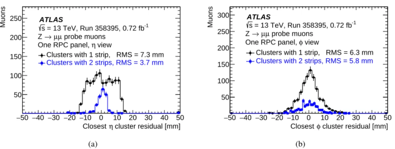
As shown in Figure5, a muon passing through an RPC module typically generates one or two hits. A cluster is defined as a set of hits in contiguous strips, with hit times that are separated by less than 12.5 ns. The size of the muon-induced clusters is an important parameter of RPC performance and is studied in Section4.2. Muon clusters are typically located close to the impact point of a muon track.

The cluster position residuals are defined as the difference between the cluster centre and the extrapolated impact point of a reconstructed muon track on the module surface. These residuals are shown in Figure6 for the representative RPC module for clusters with one or two strips. For clusters with one strip, the cluster centre is given by the strip centre and the width of the 𝜂 residual distribution is therefore determined by the strip width. This is because the 𝜂 coordinate of a muon track was measured using the MDT detector, which has much more precise 𝜂 position resolution than that of the RPC detector. For clusters with two strips, the cluster centre is defined as the midpoint between two strips. For these clusters the muon is more likely to

(12)

pass between the two strips and therefore the width of the 𝜂 residual distribution is smaller because of the slightly better estimate of the muon impact point compared to the clusters with a single hit. Muon tracks are more likely to pass close to the 𝜙 cluster centre because the 𝜙 coordinate of the muon tracks in the MS was measured using the RPC detector. Therefore, muon tracks are biased to be close to recorded 𝜙 hits, resulting in the peak near zero for the 𝜙 residual distributions. The 𝜙 residual distribution widths are similar for the clusters with one hit and with two hits because the muon track 𝜙 position uncertainty is dominated by the RPC hit position uncertainty.

cluster residual [mm] η Closest 50 − −40 −30 −20 −10 0 10 20 30 40 50 Muons 50 100 150 200 250 ATLAS -1 = 13 TeV, Run 358395, 0.72 fb s probe muons µ µ → Z view η One RPC panel,

Clusters with 1 strip, RMS = 7.3 mm Clusters with 2 strips, RMS = 3.7 mm

(a) cluster residual [mm] φ Closest 50 − −40 −30 −20 −10 0 10 20 30 40 50 Muons 50 100 150 200 250 300

Clusters with 1 strip, RMS = 6.3 mm Clusters with 2 strips, RMS = 5.8 mm

ATLAS -1 = 13 TeV, Run 358395, 0.72 fb s probe muons µ µ → Z view φ One RPC panel, (b)

Figure 6: Cluster residuals for one representative RPC module for (a) 𝜂 strips and (b) 𝜙 strips. The residuals were computed by subtracting the expected muon position from the centre of the cluster. Clusters with one strip and with two strips are shown separately. The RMS values are computed using entries with residuals between ±20 mm. No time requirements are used to select the individual RPC hits. For clusters made of two strips, the hit times are required to be within 12.5 ns of each other.

4.2 RPC detector response

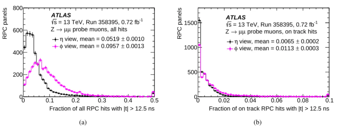
As discussed in Section 4.1, a majority of the hits recorded in a module containing the muon impact point are expected to be closely associated in time with the arrival time of that muon. RPC hit times are calibrated in order to equalise the RPC timing response for ultra-relativistic particles produced at the interaction point. A small number of out-of-time hits, defined as hits with time |𝑡 | > 12.5 ns, are also recorded, primarily due to noise and delayed signals, with a small contribution from imperfect RPC timing calibration. Figure7(a)shows the fractions of out-of-time hits for all RPC modules. These fractions were computed for each module using only those events that include a muon candidate predicted to pass through that module. The larger mean out-of-time fraction for 𝜙 hits is due to the differences between 𝜂 and 𝜙 panels described in Section2.2. The mean out-of-time fraction is reduced to about 1% when only the hits lying on the extrapolated muon track are included in the computation, as shown in Figure7(b). This result demonstrates that only a small fraction of the out-of-time muon hits originate from imperfect RPC timing calibrations.

The passage of a muon through an RPC module can produce several hits and form a cluster. Two quantities are used to study cluster properties: the cluster hit multiplicity and the cluster size. The cluster hit multiplicity is an integer distribution, with one entry corresponding to one muon candidate, where a given multiplicity bin is filled with the number of hits recorded in one event for a muon candidate passing through

(13)

Fraction of all RPC hits with |t| > 12.5 ns 0 0.1 0.2 0.3 0.4 0.5 RPC panels 0 200 400 600 800 ATLAS -1 = 13 TeV, Run 358395, 0.72 fb s

probe muons, all hits µ µ → Z 0.0010 ± view, mean = 0.0519 η 0.0013 ± view, mean = 0.0957 φ (a)

Fraction of on track RPC hits with |t| > 12.5 ns

0 0.02 0.04 0.06 0.08 0.1 RPC panels 0 500 1000 1500 ATLAS -1 = 13 TeV, Run 358395, 0.72 fb s

probe muons, on track hits µ µ → Z 0.0002 ± view, mean = 0.0065 η 0.0003 ± view, mean = 0.0113 φ (b)

Figure 7: Fraction of RPC hits with a time |𝑡 | > 12.5 ns, for (a) all hits and (b) only for hits belonging to strips with an expected muon hit. Only active RPC modules were used for these plots.

a given panel. Distributions for individual panels are added up to produce the cluster hit multiplicity distribution averaged over a collection of panels or over the entire detector. These distributions can be computed using muon candidates recorded in one run or in the entire dataset. The cluster size is defined as the mean value of the cluster hit multiplicity distribution for one panel.

The cluster hit multiplicity distribution is averaged over all RPC panels and shown in Figure8(a), computed using the full 2018 dataset. The average RPC cluster is approximately 1.5 strips wide, with the average taken separately over 𝜂 and 𝜙 panels and using all active RPC modules. The average 𝜂 panel has a cluster multiplicity which is slightly smaller than that of the average 𝜙 panel, due to the differences in the construction and readout as discussed in Section 2.2. Figure 8(b)shows the average cluster size distributions for all active RPC modules, which is computed as the mean of the cluster hit multiplicity distribution for each 𝜂 and 𝜙 panel. There are some 𝜂 panels that have larger-than-typical cluster sizes, seen as the tail of the 𝜂 distribution in Figure8(b).

RPC cluster multiplicity in response to muons [strips]

0 5 10 Fraction of muons 0 0.1 0.2 0.3 0.4 0.5 0.6 0.7 0.8 0.9 1 ATLAS -1 = 13 TeV, Data 2018, 60.8 fb s probe muons µ µ → Z

Combined cluster multiplicity over all RPC modules view, mean = 1.430 η view, mean = 1.452 φ (a)

Mean RPC module cluster size [strips]

1 2 3 4 Modules 0 500 1000 1500 ATLAS -1 = 13 TeV, Data 2018, 60.8 fb s probe muons µ µ → Z All RPC modules view, mean = 1.450 η view, mean = 1.431 φ (b)

Figure 8: (a) RPC cluster hit multiplicity distribution and (b) RPC cluster size distribution, both averaged over all modules, in response to the passage of a muon through a module, with 𝜂 and 𝜙 panels shown separately.

(14)

The cluster hit multiplicity distribution averaged over the entire RPC detector is given in Table1. Muons produce clusters with two or more hits in 30% and 36% of events for the 𝜂 and 𝜙 panels, respectively. Larger clusters containing four or more hits are produced in 2.7% and 1.6% of events for the 𝜂 and 𝜙 panels, respectively. Variations in the cluster hit multiplicity are due to the differences between 𝜂 and 𝜙 panels described in Section2.2and to small differences in strip widths.

Table 1: Cluster hit multiplicity distribution in response to a passage of a muon, shown separately for 𝜂 and 𝜙 panels. These multiplicity distributions are summed over all active RPC modules, separately for 𝜂 and 𝜙 panels. The statistical uncertainty for all table entries is smaller than 0.1%.

Cluster hit multiplicity 1 2 3 4 5 > 5 𝜂_panels _70.5% _21.0% _5.9% _1.6% _0.6% _0.5% 𝜙_panels _64.1% _29.6% _4.6% _1.0% _0.3% _0.3%

RPC cluster multiplicity in response to muons [strips]

0 5 10 Fraction of muons 0 0.2 0.4 0.6 0.8 1 1.2 1.4 ATLAS -1 = 13 TeV, Run 358395, 0.72 fb s probe muons µ µ → Z = 1.0 V thr V view, η φ view, V_thr = 1.0 V > 1.0 V thr V view, η > 1.0 V thr V view, φ

Combined cluster multiplicity over all selected RPC modules

(a)

Mean RPC module cluster size [strips]

1 2 3 4 Modules 500 1000 1500 2000 ATLAS -1 = 13 TeV, Run 358395, 0.72 fb s probe muons µ µ → All RPC modules, Z = 1.0 V thr V view, η φ view, V_thr = 1.0 V > 1.0 V thr V view, η > 1.0 V thr V view, φ (b)

Figure 9: (a) Cluster hit multiplicity and (b) cluster size distributions for all selected modules shown separately for 𝜂 and 𝜙 panels using nominal (𝑉thr= 1.0 V) and higher than nominal (𝑉thr >1.0 V) FE thresholds.

To illustrate the effect of the FE thresholds on the RPC cluster size, the cluster hit multiplicity distribution and cluster size were measured separately for panels with nominal FE thresholds and for panels with FE thresholds higher than their nominal values. One typical ATLAS run was analysed for this study. In this run, the majority of the panels utilised the default FE threshold setting of 𝑉thr = 1.0 V. A small fraction

of the panels utilised higher-than-nominal FE thresholds that varied in the range from 𝑉thr = 1.1 V to

𝑉

thr= 1.5 V in steps of 0.1 V. These results are shown in Figure9separately for the 𝜂 and 𝜙 panels. As

expected, higher FE thresholds result in smaller cluster hit multiplicity and smaller cluster sizes.

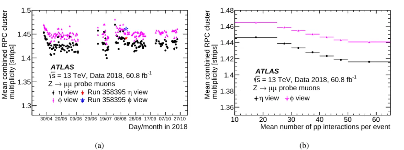
The average cluster hit multiplicity was monitored as a function of time, as shown in Figure10(a)where each entry corresponds to one ATLAS run. The small variations among runs are due to changes in the FE thresholds and changes in the detector conditions, such as automatic adjustments of the applied voltage. Overall, the mean RPC cluster multiplicity was stable in 2018 to within a few percent. The small decrease in the cluster multiplicity in late April and early May was due to operating the RPCs at nominal voltage with collisions following the winter LHC shutdown when the RPC voltage was off. The small increase in August was due to adjustments of the FE thresholds, leading to the slightly larger detector efficiency described in Section4.3.

(15)

Day/month in 2018 30/04 20/05 09/06 29/06 19/07 08/08 28/08 17/09 07/10 27/10

multiplicity [strips]

Mean combined RPC cluster

1.3 1.35 1.4 1.45 1.5 ATLAS -1 = 13 TeV, Data 2018, 60.8 fb s probe muons µ µ → Z view η Run 358395 η view view φ Run 358395 φ view (a)

Mean number of pp interactions per event

10 20 30 40 50 60

multiplicity [strips]

Mean combined RPC cluster

1.36 1.38 1.4 1.42 1.44 1.46 1.48 ATLAS -1 = 13 TeV, Data 2018, 60.8 fb s probe muons µ µ → Z view η φ view (b)

Figure 10: Mean of the RPC detector cluster hit multiplicity distribution plotted (a) as a function of time and (b) as a function of average number of proton–proton collisions per event. Mean values for 𝜂 and 𝜙 panels are shown separately. The blue and red stars refer to the representative run used in most of the performance studies shown in this paper.

interactions per event. An instantaneous luminosity of 2 × 1034cm−2s−1corresponds on average to about 56 collisions per event. A reduction of approximately 1% to 2% between the first and last bins was observed. This small reduction is due to dead time imposed by the readout system and to offline reconstruction in each individual strip, in addition to a small chamber inefficiency at higher detector occupancy [36,37]. If a strip records a hit due to a background event, then a later muon hit within the dead-time window will be discarded, thereby introducing a small inefficiency in that channel. These background hits would decrease both the mean cluster size and also the muon detection efficiency, as shown in Section4.3.

4.3 RPC detector performance

The RPC efficiency for muon-induced signals is shown in Figure11(a)for all RPC modules without known defects using data from one representative ATLAS run. The efficiency is computed using signal hits, defined in Section4.1. The efficiency for 𝜂 and 𝜙 panels belonging to the same module is computed independently by requiring at least one hit in 𝜂 or 𝜙 strips, respectively. The module (gas gap) efficiency is computed by requiring at least one hit either in 𝜂 or 𝜙 strips belonging to the same module. The gap efficiency corresponds to the intrinsic RPC efficiency to detect a muon-induced avalanche. The 𝜂/𝜙 panel efficiency includes the efficiency for the FE electronics to register the avalanche signal, which is estimated from the difference between the module efficiency and 𝜂/𝜙 panel efficiency to be approximately 97%. The RPC detector efficiency is plotted as a function of time in Figure11(b), which shows the 𝜂/𝜙 panel efficiency and gas gap efficiency. The mean detector efficiency in each ATLAS run is computed by averaging over all active RPC modules with efficiency greater than 50%, which represent about 90% of the total number of modules. A small increase in the average efficiency of about 0.3% in August 2018 was due to adjustments of FE thresholds. No significant ageing effects have been observed during 2018 while the ATLAS detector recorded approximately 60.8 fb−1of proton–proton collision data.

The module efficiency is shown in Figure12for all modules in the first and second layers of the RPC1 doublet layer. The red bins indicate modules with low efficiency or modules with the operating voltage off due to gas leaks. Inefficient modules had only a small impact on the muon trigger efficiency because

(16)

Efficiency 0.5 0.6 0.7 0.8 0.9 1 Gaps, panels/0.01 200 400 600 800 1000 1200 panels, mean = 0.910 η panels, mean = 0.914 φ

Gas gaps, mean = 0.948

ATLAS -1 = 13 TeV, Run 358395, 0.72 fb s probe muons µ µ → Z |t| < 12.5 ns, |d| < 30 mm (a) Day/month in 2018 30/04 20/05 09/06 29/06 19/07 08/08 28/08 17/09 07/10 27/10

Mean RPC detector efficiency

0.82 0.84 0.86 0.88 0.9 0.92 0.94 0.96 ATLAS -1 = 13 TeV, Data 2018, 60.8 fb s

Mean of all RPC modules probe muons µ µ → Z |t| < 12.5 ns, |d| < 30 mm view η φ view gap (b)

Figure 11: (a) Distribution of the muon detection efficiency for all active RPC modules. (b) Muon detection efficiency for 𝜂 panels, 𝜙 panels and gaps averaged over all active RPC modules plotted as a function of time.

muons producing a single hit in the two layers can still satisfy the trigger logic requirements, as discussed in Section5.1. index η 8 − −7−6−5−4−3−2−10 1 2 3 4 5 6 7 8 sector φ L1 S2 L3 S4 L5 S6 L7 S8 L9 S10L11 FG12 L13 FG14 L15 S16 _∈gap 0 0.2 0.4 0.6 0.8 1 -1 = 13 TeV, 0.72 fb s , Run 358395, ATLAS

probe muons, RPC1, gas gap 1 µ µ → Z (a) index η 8 − −7−6−5−4−3−2−10 1 2 3 4 5 6 7 8 sector φ L1 S2 L3 S4 L5 S6 L7 S8 L9 S10L11 FG12 L13 FG14 L15 S16 _∈gap 0 0.2 0.4 0.6 0.8 1 -1 = 13 TeV, 0.72 fb s , Run 358395, ATLAS

probe muons, RPC1, gas gap 2 µ

µ → Z

(b)

Figure 12: Muon detection efficiency in the 𝜂–𝜙 plane for all modules in (a) the first layer and (b) the second layer of the RPC1 doublet layer. Modules within one station are represented using half-integer values of 𝜂 index and 𝜙 sector. Empty bins correspond to logical combinations of indices that do not represent installed RPCs.

The muon detection efficiency is shown in Figure13as a function of the mean number of proton–proton interactions per event. The detector efficiency is reduced by approximately 1% over the range considered for the reasons discussed in Section4.2. The dependence of the detector efficiency on detector occupancy is investigated further in Section6.4.

One potential bias in measuring the efficiency of 𝜙 panels can arise from the offline reconstruction of muon candidates, which uses RPCs to measure the 𝜙 coordinates of muon tracks in the MS. The RPC detector provides up to six 𝜂 and 𝜙 position measurements for each muon track. Therefore, the impact of a single RPC detector layer on the muon detection efficiency is expected to be negligible. This hypothesis was first checked by extrapolating ID tracks to the RPC detector surfaces. No detectable biases were observed for

(17)

Mean number of pp interactions per event

10 20 30 40 50 60

Mean RPC detector efficiency

0.895 0.9 0.905 0.91 0.915 0.92 0.925 0.93 ATLAS -1 = 13 TeV, Data 2018, 60.8 fb s probe muons µ µ → Z |t| < 12.5 ns, |d| < 30 mm view η φ view

Figure 13: Muon detection efficiency for 𝜂 and 𝜙 panels, averaged over all active RPC modules, plotted as a function of average number of proton–proton collisions per event.

the measurements reported in this section when using this alternative extrapolation algorithm. This effect was also checked by comparing the efficiencies of the 𝜂 panel and 𝜙 panel belonging to the same RPC module. The average difference between the 𝜂 and 𝜙 efficiencies is consistent with zero, confirming that no significant bias was introduced by using RPCs for reconstructing 𝜙 positions of muon tracks in the MS.

4.4 Time resolution of RPC detector and readout system

The RPC technology was chosen by the ATLAS experiment for the L1 muon barrel trigger because of its fast response, good time and position resolution, and relatively low cost [19]. Before the construction of the ATLAS detector, the RPC time resolution was measured using full-size prototype units of the ATLAS RPCs equipped with the final version of the FE electronics [38]. The time resolution was measured to be around 1.1 ns without an irradiation source and 1.4 ns with a gamma irradiation source enabled [38]. The time resolution of the installed RPC detectors was measured using muons produced in proton–proton collisions recorded in 2011 at a centre-of-mass energy of 7 TeV. A time resolution value of around 2 ns was obtained [39]. This higher value, compared to the results from test-beam facilities, was due to combined effects of the RPC intrinsic resolution and the readout system resolution.

In this section, the intrinsic time resolution of the RPC detector and the time resolution of RPC electronics are evaluated separately using newly developed procedures for the analysis of the RPC timing response to probe muons produced in the decays of 𝑍 bosons, with the selection criteria detailed in Section3. These results aim to quantify the RPC intrinsic time resolution for detecting a signal induced by an ionising particle, excluding effects related to the resolution of its absolute arrival time. The intrinsic RPC time resolution depends on fluctuations in the location of the first ionisation event along the muon path through the RPC gas gap and on the statistical fluctuations inherent in the subsequent avalanche amplification process [40]. The electronics time resolution component includes several sources, such as the 320 MHz sampling frequency and the associated jitter [22]. The total time resolution (𝜎total) of an RPC is defined as:

𝜎2 total= 𝜎 2 intrinsic+ 𝜎 2 electronics (1)

where 𝜎intrinsicis the component corresponding to the intrinsic RPC time resolution and 𝜎electronicsis the

(18)

The total RPC time resolution was estimated using time differences between detector signals generated by the same muon passing through two parallel single RPC layers belonging to the same module. These two layers are separated by a distance of approximately 20 mm. The time difference was computed using hits produced in the two parallel strips (either a pair of 𝜂 strips or a pair of 𝜙 strips) that are closest to the muon track in each of the two detector layers. A relativistic muon travelling nearly at the speed of light will produce a time-of-flight difference of about 0.07 ns when travelling perpendicular to the two detector layers. Since the contribution from the muon time-of-flight component is negligible, the time differences between signals produced in the two layers are dominated by the total RPC time resolution.

The time-difference distributions were obtained for all geometrically possible combinations of 𝜂 strip pairs and 𝜙 strip pairs in each doublet layer of the RPC detector. The same timing circuit was used to measure these two signals so no differences are introduced due to clock synchronisation. Only distributions with at least 100 entries were selected for the analysis in order to remove strips with low efficiency. The width of the time-difference distribution was determined from a binned maximum-likelihood fit of a Gaussian function to the observed distribution of time differences. An example fit is shown in Figure14(a)for a pair of 𝜂 strips from the two parallel layers of one RPC chamber. The Kolmogorov–Smirnov (KS) test was performed to assess the goodness of fit. To perform this test, a new histogram was generated with the number of entries in each bin equal to the area of the Gaussian curve in that bin divided by the bin width. Only strip pair distributions with a KS probability greater than 0.1 and with at least three non-empty bins were retained for the final analysis. These selection criteria have a combined efficiency of about 98%.

10 − −5 0 5 10 [ns] η layer 1 - t η layer 0 RPC t 0 100 200 300 400 Muons/3.125 ns ATLAS -1 = 13 TeV, 60.8 fb s 0.12 ns ± Fitted mean = 0.26 0.09 ns ± = 1.92 fit, total σ Fitted width = Data Gaussian fit Expected entries from fit

(a) 0 2 4 6 8 10 [ns] fit, total σ 0 2000 4000 6000 8000 10000

RPC readout strip pairs/0.1 ns

ATLAS -1 = 13 TeV, 60.8 fb s fit, total σ Fitted width = view, mean = 2.06 ns η view, mean = 2.21 ns φ (b)

Figure 14: (a) Time-difference distribution between signals generated by the same muon in a single pair of 𝜂 strips, matched with the muon track, in two parallel RPC detector layers. The bin width corresponds to the 3.125 ns sampling time. (b) Distribution of the total time differences for the all selected RPC strip pairs.

The best-fit Gaussian widths for all selected 𝜂 strip pairs and 𝜙 strip pairs are shown in Figure14(b)for the full RPC system. The mean width of the time differences is approximately 2.1 ns and 2.2 ns for 𝜂 and 𝜙 strips, respectively. The small difference between the 𝜂 and 𝜙 strips is due to the different cluster size distributions for 𝜂 and 𝜙 panels, which is discussed in Section4.2. When the time differences were measured using only those muons that produce clusters with a single hit in both layers, no difference between 𝜂 and 𝜙 strips was observed for the time difference widths.

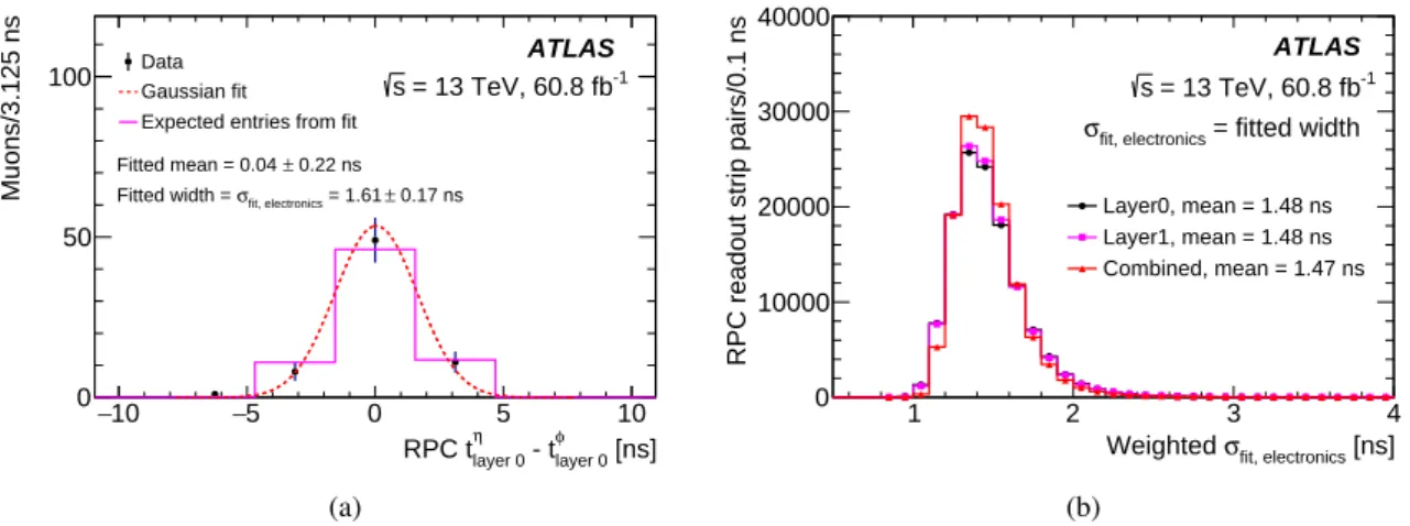
The electronic component of the time resolution was estimated by taking the difference between time measurements of simultaneous 𝜂 and 𝜙 hits from the same avalanche event induced by a muon passing

(19)

10 − −5 0 5 10 [ns] φ layer 0 - t η layer 0 RPC t 0 50 100 Muons/3.125 ns ATLAS -1 = 13 TeV, 60.8 fb s 0.22 ns ± Fitted mean = 0.04 0.17 ns ± = 1.61 fit, electronics σ Fitted width = Data Gaussian fit Expected entries from fit

(a) 1 2 3 4 [ns] fit, electronics σ Weighted 0 10000 20000 30000 40000

ATLAS -1 = 13 TeV, 60.8 fb s = fitted width fit, electronics σ Layer0, mean = 1.48 ns Layer1, mean = 1.48 ns Combined, mean = 1.47 ns (b)

Figure 15: (a) Time-difference distribution between signals generated by the same muon in a single pair of 𝜂 and 𝜙 strips, matched with the muon track, belonging to one detector layer. (b) Distribution of the electronic component of the time resolution.

through a single detector layer. The intrinsic RPC resolution cancels out in this measurement because the same avalanche event is observed by a pair of 𝜂 and 𝜙 strips. Two different timing circuits were used to measure these two signals but since their clocks are synchronised to the same LHC reference clock, any differences in clock synchronisation would produce a shift of the mean of the time-difference distribution but leave its width unchanged.

The time-difference distribution was computed for each pair of orthogonal 𝜂 and 𝜙 strips observing the same avalanche event in the common gas volume. Delays due to different strip and cable lengths result in a constant offset of the mean value of this time-difference distribution. The width of this time-difference distribution is then proportional to the electronics time resolution. A binned maximum-likelihood fit to a Gaussian function was performed for each time-difference distribution. Only distributions with at least 20 entries were selected in order to remove strip pairs with low efficiency. An example fit is shown in Figure15(a). The KS test was performed to assess the goodness of fit. Only strip pair distributions with a KS probability greater than 0.4 and with at least three non-empty bins were retained for the final analysis, with the later criterion removing the majority of strip pairs. These selection criteria have a combined efficiency of about 75%.

All possible combinations of 𝜂 and 𝜙 strip pairs were considered in each layer of each module for the full RPC system. For each 𝜂 (𝜙) strip, several combinations with orthogonal 𝜙 (𝜂) strips can be made. The electronics time resolution component associated with each single strip is therefore estimated as the statistically weighted average among all possible combinations with the orthogonal strips, where each individual measurement was weighted by the inverse of the square of the uncertainty in the fitted value of the Gaussian width parameter. Figure15(b)shows the distribution of the best-fit Gaussian widths of the time-difference distributions for the full RPC system. The results for two layers for each module were combined for the estimate of the intrinsic time resolution component using the same weighting procedure, since both layers were used in the total time resolution measurements.

Finally, the intrinsic component of the time resolution was estimated using Eq. (1). The resulting distributions are shown in Figure16for all selected 𝜂 and 𝜙 strip pairs. The mean values of the distributions should be divided by

√

(20)

0 2 4 6 8 10 [ns] 2 fit, electronics σ - 2 fit, total σ 0 2000 4000 6000 8000

ATLAS -1 = 13 TeV, 60.8 fb s view, mean = 1.44 ns η view, mean = 1.64 ns φ

Figure 16: Distribution of the intrinsic component of the time resolution for 𝜂 and 𝜙 panels.

the resulting intrinsic time resolution is consistent with the previous measurements obtained at test-beam facilities.

5 Performance of L1 muon barrel trigger

This section reports measurements of the L1 muon barrel trigger performance obtained using proton–proton collision data. Section5.1studies the performance of individual trigger towers. Section 5.2presents measurements of the L1 muon barrel trigger efficiency as a function of several quantities. The measurements in these two sections were performed using events containing a 𝑍 boson decay into a pair of muons. Section5.3presents measurements of the L1 muon trigger’s event selection rate as a function of the instantaneous luminosity. Finally, Section5.4studies the composition of the events selected by the L1 muon barrel trigger.

5.1 Trigger roads

Processing of signals (hits) produced by the RPC FE electronics is first performed by the on-detector electronics contained in the processor box (PAD) [22]. Each PAD contains four coincidence matrices, with each matrix implemented in one application-specific integrated circuit, referred to as CMA. These custom-designed circuits perform digital signal shaping, set a programmable dead time, mask channels and perform trigger logic operations. The CMA trigger logic aligns the FE signals in time, checks the time coincidence of RPC hits, and applies the geometrical matching criteria for selecting one of the three programmable 𝑝T thresholds. Two types of PADs are deployed: one is responsible for the low-𝑝Ttrigger

and another is responsible for the high-𝑝T trigger. In each PAD, two CMAs collect the signals from the

𝜂_{view strips and another two CMAs collect the signals from the 𝜙 view strips. Each RPC PAD covers} an 𝜂 × 𝜙 detector region of approximately 0.2 × 0.2, with the overlap of one 𝜙 CMA and one 𝜂 CMA corresponding to a single RoI of approximately 0.1 × 0.1. Two PADs, one for the low-𝑝T trigger and one

for the high-𝑝Ttrigger, make one trigger tower. A set of six, seven or eight trigger towers, placed along the

𝑧_{-axis at a fixed 𝜙 position, makes one trigger sector. There are in total 432 trigger towers, divided in 64} azimuthal trigger sectors, with 32 sectors on each ATLAS side.

(21)

CMAs identify muon candidates and measure their momentum by searching for geometrical matching of RPC hits inside programmable windows, called trigger roads, defined using the detector strips, as illustrated in Figure 3 of Ref. [41]. A muon candidate satisfies the L1 barrel trigger logic conditions if it generates RPC hits inside the trigger roads for a matching pair of 𝜂 and 𝜙 CMAs. The low-𝑝T(high-𝑝T) trigger

checks for coincident RPC signals between the pivot RPC2 and RPC1 (RPC3) doublet layers within the corresponding trigger road. The low-𝑝T(high-𝑝T) trigger also requires signals in three out of four (one out

of two) RPC detector layers, in both the 𝜂 and 𝜙 views. The trigger roads were defined to contain 95% of positively and negatively charged muons, simulated using the ATLAS simulation infrastructure [42] with a fixed 𝑝Tvalue equal to the trigger 𝑝Tthreshold. Trigger roads encode the RPC detector layout, magnetic

field configuration, and geometric relationships among strips in the different layers, as seen by a muon travelling from the interaction region.

Table 2: List of the hit selection criteria used to evaluate the performance of each individual CMA.

Type CMA type Selection criteria Muon kinematics Low 𝑝T 𝑝T ≥ 10 GeV, |𝜂| ≤ 1.05

High 𝑝T 𝑝T ≥ 20 GeV, |𝜂| ≤ 1.05

Time | 𝑡pivot layer channel− 𝑡confirm layer channel| ≤ 12.5 ns

Layer Low 𝑝T 𝑁pivot layers with hits+ 𝑁confirm layers with hits≥ 3

High 𝑝T 𝑁pivot layers with hits ≥ 1, 𝑁confirm layers with hits≥ 1

Hit multiplicity Low 𝑝T 𝑁hits in pivot layer ≤ 4, 𝑁hits in confirm layer ≤ 4

High 𝑝T 𝑁hits in pivot layer ≤ 2, 𝑁hits in confirm layer ≤ 4

The performance of each individual CMA was evaluated using probe muons produced in decays of the 𝑍 bosons. Probe muons were matched with the four closest CMAs by requiring the angular Δ𝑅 distance between the muon track and the centre of the CMA to be less than 0.15. The MU10 (MU20) trigger roads were evaluated using offline muon candidates with 𝑝T > 10 (20) GeV. Signals in the confirm layer were

required to be within the 25 ns time window centred at the pivot signal time, thereby requiring the selected signals to belong to the same bunch crossing. To reduce contributions from background events due to random coincidences, at least three out of four layers of RPC1 and RPC2 were required to contain signals in the selected low-𝑝T CMA. Similarly, at least one of the two layers of RPC3 was required to contain

signals in the selected high-𝑝TCMA. These two selection criteria approximate similar conditions applied

by the on-detector PAD electronics [22]. Finally, events with more than four signals in one detector layer were removed to reduce the number of combinations between the pivot and confirm layers. These selection criteria are summarised in Table2.

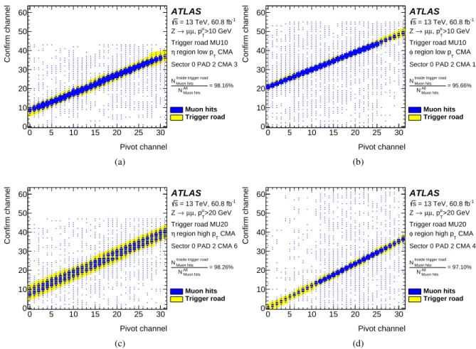
Figure 17shows the selected RPC hits in the pivot and confirm layers for four representative CMAs belonging to the same PAD: low- and high-𝑝TCMAs in both the 𝜂 and 𝜙 views. For each hit in the pivot

layer, all possible combinations with the selected hits in the confirm layer are reported. The trigger roads used for 2018 data-taking are shown in yellow. As expected, the majority of hits are produced by the probe muons and are contained within the trigger roads.

The fractions of the selected RPC hit pairs inside the trigger roads (referred to as trigger road hit fractions) were computed for all CMAs in order to study the trigger road performance using the actual detector.

(22)

0 5 10 15 20 25 30 Pivot channel 0 10 20 30 40 50 60 Confirm channel ATLAS -1 = 13 TeV, 60.8 fb s >10 GeV µ T , p µ µ → Z

Trigger road MU10 CMA T region low p η

Sector 0 PAD 2 CMA 3

= 98.16% All

Muon hits N Inside trigger road Muon hits N Muon hits Trigger road (a) 0 5 10 15 20 25 30 Pivot channel 0 10 20 30 40 50 60 Confirm channel ATLAS -1 = 13 TeV, 60.8 fb s >10 GeV µ T , p µ µ → Z

Trigger road MU10 CMA T region low p φ

= 95.66% All

Muon hits N Inside trigger road Muon hits N Muon hits Trigger road (b) 0 5 10 15 20 25 30 Pivot channel 0 10 20 30 40 50 60 Confirm channel ATLAS -1 = 13 TeV, 60.8 fb s >20 GeV µ T , p µ µ → Z

Trigger road MU20 CMA T region high p η

= 98.26% All

Muon hits N Inside trigger road Muon hits N Muon hits Trigger road (c) 0 5 10 15 20 25 30 Pivot channel 0 10 20 30 40 50 60 Confirm channel ATLAS -1 = 13 TeV, 60.8 fb s >20 GeV µ T , p µ µ → Z

Trigger road MU20 CMA T region high p φ

= 97.10% All

Muon hits N Inside trigger road Muon hits N

Muon hits Trigger road

(d)

Figure 17: L1 muon barrel trigger roads for four example CMAs: (a) MU10 low-𝑝T𝜂CMA, (b) MU10 low-𝑝T𝜙 CMA, (c) MU20 high-𝑝T𝜂CMA, (d) MU20 high-𝑝T𝜙CMA.

Figures18(a)and18(b)show the number of probe muons passing through each CMA and the trigger road hit fractions for each CMA, respectively. Typically, several hundred probe muons pass through each CMA, providing sufficient precision to study the performance of the trigger roads.

Figure19shows the distributions of the trigger road hit fractions for the MU10 and MU20 triggers for all CMAs. In events with probe muons passing through the CMA, more than 95% of the selected pivot and confirm hit pairs are contained within the trigger road. The trigger road hit fractions are larger than 95% for the majority of CMAs, indicating good performance of the MU10 and MU20 triggers. These fractions are slightly larger for the 𝜂 CMAs than for the 𝜙 CMAs because the trigger roads were defined to contain 95% of muons with 𝑝T= 20 GeV while the majority of the probe muons have 𝑝Tbetween 30 and 50 GeV.

Therefore, probe muon trajectories in the bending 𝜂 view have a slighter higher probability to fall within the trigger road than in the non-bending 𝜙 view. Approximately 2% of 𝜂 CMAs and 4% of 𝜙 CMAs have trigger road hit fractions below 90%. These lower fractions are due to residual differences between the actual and simulated detector geometries.

(23)

0 10 20 30 40 50 60 Sector number 0 10 20 30 40 50 60

PAD number x 10 + CMA number

0 500 1000 1500 2000 2500 3000 3500 4000

pivot-confirm pair of trigger road

Average muon hits in single

occupancy for MU10/MU20 trigger roads L1 muon barrel trigger, average muon

-1 = 13 TeV, 60.8 fb s ATLAS (a) 0 10 20 30 40 50 60 Sector number 0 10 20 30 40 50 60

PAD number x 10 + CMA number

0 10 20 30 40 50 60 70 80 90 100

Fraction of muon hits inside trigger road [%]

L1 muon barrel trigger, MU10/MU20 trigger road -1 = 13 TeV, 60.8 fb s ATLAS (b)

Figure 18: (a) Average number of the probe muons passing through each CMA and (b) fraction of the selected RPC hits inside the trigger road for each CMA. The horizontal axis corresponds to the trigger sector number. The vertical axis shows the PAD number multiplied by 10 plus the CMA number. Low-𝑝TCMA numbers range from 0 to 3 and high-𝑝TCMA numbers range from 4 to 7. The trigger roads employed for this study correspond to the MU10 and MU20 triggers for the low-𝑝Tand high-𝑝TCMAs, respectively.

50 55 60 65 70 75 80 85 90 95 100

Muon hits inside trigger road (%) 1 10 2 10 Number of CMA region CMAs η region CMAs φ ATLAS -1 = 13 TeV, 60.8 fb s >10 GeV µ T , p µ µ → Z

Trigger road MU10 CMAs

T

Low p

(a)

50 55 60 65 70 75 80 85 90 95 100

Muon hits inside trigger road (%) 1 10 2 10 Number of CMA region CMAs η region CMAs φ ATLAS -1 = 13 TeV, 60.8 fb s >20 GeV µ T , p µ µ → Z

Trigger road MU20 CMAs

T

High p

(b)

Figure 19: Distributions of the fraction of selected RPC hits inside the trigger road for the (a) MU10 and (b) MU20 triggers, shown separately for 𝜂 and 𝜙 CMAs.

5.2 Trigger efficiency and timing

The efficiency of the L1 muon barrel trigger to detect a probe muon was evaluated as a function of several parameters. Figure20shows the trigger efficiency as a function of probe muon 𝜂 and 𝜙 for the MU10 and MU20 triggers. Only muons with 𝑝T >25 GeV were used for these measurements; this removes the

dependence of the trigger efficiency on the muon 𝑝T. Regular features in the trigger efficiency distributions

correspond to the ATLAS detector support structures and service elements. The drop in the trigger efficiency at 𝜂 ∼ 0 in Figure20(a)is due to the presence of detector services, such as gas pipes, water pipes, cryogenic lines, and cables, which cause the region |𝜂| < 0.1 to be only sparsely instrumented with RPCs. Other, smaller efficiency drops, mainly at |𝜂| ∼ 0.4 and |𝜂| ∼ 0.8, are due to the presence of the