Search for new phenomena in high-mass final states with a photon and a jet from $pp$ collisions at $\sqrt{s}$ = 13 TeV with the ATLAS detector

EUROPEAN ORGANISATION FOR NUCLEAR RESEARCH (CERN)

Submitted to: EPJC CERN-EP-2017-148

2nd October 2017

Search for new phenomena in high-mass final states

with a photon and a jet from pp collisions at

√

s

=

13 TeV with the ATLAS detector

The ATLAS Collaboration

A search is performed for new phenomena in events having a photon with high transverse momentum and a jet collected in 36.7 fb−1 of proton–proton collisions at a centre-of-mass energy of √s= 13 TeV recorded with the ATLAS detector at the Large Hadron Collider. The invariant mass distribution of the leading photon and jet is examined to look for the reson-ant production of new particles or the presence of new high-mass states beyond the Stand-ard Model. No significant deviation from the background-only hypothesis is observed and cross-section limits for generic Gaussian-shaped resonances are extracted. Excited quarks hypothesized in quark compositeness models and high-mass states predicted in quantum black hole models with extra dimensions are also examined in the analysis. The observed data exclude, at 95% confidence level, the mass range below 5.3 TeV for excited quarks and 7.1 TeV (4.4 TeV) for quantum black holes in the Arkani-Hamed–Dimopoulos–Dvali (Randall–Sundrum) model with six (one) extra dimensions.

c

2017 CERN for the benefit of the ATLAS Collaboration.

Reproduction of this article or parts of it is allowed as specified in the CC-BY-4.0 license.

1 Introduction

This paper reports a search for new phenomena in events with a photon and a jet produced from proton– proton (pp) collisions at √s= 13 TeV, collected with the ATLAS detector at the Large Hadron Collider (LHC). Prompt photons in association with jets are copiously produced at the LHC, mainly through quark–gluon scattering (qg → qγ). The γ + jet(s) final state provides a sensitive probe for a class of phenomena beyond the Standard Model (SM) that could manifest themselves in the high invariant mass (mγ j) region of the γ+ jet system. The search is performed by looking for localized excesses of events in the mγ j distribution with respect to the SM prediction. Two classes of benchmark signal models are considered.

The first class of benchmark models is based on a generic Gaussian-shaped mass distribution with differ-ent values of its mean and standard deviation. This provides a generic interpretation for the presence of signals with different Gaussian widths, ranging from a resonance with a width similar to the reconstruc-ted mγ j resolution of ∼ 2% to wide resonances with a width up to 15%. The second class of benchmark models is based on signals beyond the SM that are implemented in Monte Carlo (MC) simulation and ap-pear as broad peaks in the mγ j spectrum. This paper considers two scenarios for physics beyond the SM: quarks as composite particles and extra spatial dimensions. In the first case, if quarks are composed of more fundamental constituents bound together by some unknown interaction, new effects should appear depending on the value of the compositeness scaleΛ. In particular, if Λ is sufficiently smaller than the centre-of-mass energy, excited quark (q∗) states may be produced in high-energy pp collisions at the LHC [1–3]. The q∗production at the LHC could result in a resonant peak at the mass of the q∗(mq∗) in the m_{γ j}

distribution if the q∗ can decay into a photon and a quark (qg → q∗ → qγ). In the present search, only the SM gauge interactions are considered for q∗production. In the second scenario, the existence of extra spatial dimensions (EDs) is assumed to provide a solution to the hierarchy problem [4–6]. Certain types of ED models predict the fundamental Planck scale M∗in the 4+ n dimensions (n being the number of extra spatial dimensions) to be at the TeV scale, and thus accessible in pp collisions at √s= 13 TeV at the LHC. In such a TeV-scale M∗scenario of the extra dimensions, quantum black holes (QBHs) may be pro-duced at the LHC as a continuum above the threshold mass (Mth) and then decay into a small number of

final-state particles including photon–quark/gluon pairs before they are able to thermalize [7–10]. In this case a broad resonance-like structure could be observed just above Mthon top of the SM mγ jdistribution.

The Mth value for QBH production is taken to be equal to M∗while the maximum allowed QBH mass

is set to either 3M∗or the LHC pp centre-of-mass energy of 13 TeV, whichever is smaller. The upper bound on the mass ensures that the QBH production is far from the “thermal” regime, where the classical description of the black hole and its decay into high-multiplicity final states should be used. In this paper, the extra-dimensions model proposed by Arkani-Hamed, Dimopoulous and Dvali (ADD) [11] with n= 6 flat EDs and the one by Randall and Sundrum (RS1) [12] with n= 1 warped ED are considered.

The ATLAS and CMS experiments at the LHC have performed searches for excited quarks in the γ+ jet final state using pp collision data recorded at √s = 7 TeV [13], 8 TeV [14, 15] and 13 TeV [16]. In the ATLAS searches, limits for generic Gaussian-shaped resonances were obtained at 7, 8 and 13 TeV while a limit for QBHs in the ADD model (n = 6) was first obtained at 8 TeV. The ATLAS search at 13 TeV with data taken in 2015 was further extended to constrain QBHs in the RS1 model (n= 1). No significant excess of events was observed in any of these searches, and the lower mass limits of 4.4 TeV for the q∗and 6.2 (3.8) TeV for QBHs in the ADD (RS1) model were set, currently representing the most stringent limits for the decay into a photon and a jet. For a Gaussian-shaped resonance a cross-section

upper limit of 0.8 (1.0) fb at √s= 13 TeV was obtained, for example, for a mass of 5 TeV and a width of 2% (15%).

The dijet resonance searches at ATLAS [17,18] and CMS [19] using pp collisions at √s= 13 TeV also set limits on the production cross-sections of excited quarks and QBHs. The search in the γ+ jet final state presented here complements the dijet results and provides an independent check for the presence of these signals in different decay channels.

This paper presents the search based on the full 2015 and 2016 data set recorded with the ATLAS detector, corresponding to 36.7 fb−1of pp collisions at √s= 13 TeV. The analysis strategy is unchanged from the one reported in Ref. [16], focusing on the region where the γ+ jet system has a high invariant mass. The paper is organized as follows. In Section 2 a brief description of the ATLAS detector is given. Section3summarizes the data and simulation samples used in this study. The event selection is discussed in Section4. The signal and background modelling are presented in Section5together with the signal search and limit-setting strategies. Finally the results are discussed in Section6and the conclusions are given in Section7.

2 ATLAS detector

The ATLAS detector at the LHC is a multi-purpose, forward-backward symmetric detector1with almost full solid angle coverage, and is described in detail elsewhere [20, 21]. Most relevant for this analysis are the inner detector (ID) and the calorimeter system composed of electromagnetic (EM) and hadronic calorimeters. The ID consists of a silicon pixel detector, a silicon microstrip tracker and a transition ra-diation tracker, all immersed in a 2 T axial magnetic field, and provides charged-particle tracking in the range |η| < 2.5. The electromagnetic calorimeter is a lead/liquid-argon (LAr) sampling calorimeter with accordion geometry. The calorimeter is divided into a barrel section covering |η| < 1.475 and two endcap sections covering 1.375 < |η| < 3.2. For |η| < 2.5 it is divided into three layers in depth, which are finely segmented in η and φ. In the region |η| < 1.8, an additional thin LAr presampler layer is used to correct for fluctuations in the energy losses in the material upstream of the calorimeters. The hadronic calorimeter is a sampling calorimeter composed of steel/scintillator tiles in the central region (|η| < 1.7), while cop-per/LAr modules are used in the endcap (1.5 < |η| < 3.2) regions. The forward region (3.1 < |η| < 4.9) is instrumented with copper/LAr and tungsten/LAr calorimeter modules optimized for electromagnetic and hadronic measurements, respectively. Surrounding the calorimeters is a muon spectrometer that includes three air-core superconducting toroidal magnets and multiple types of tracking chambers, providing pre-cision tracking for muons within |η| < 2.7 and trigger capability within |η| < 2.4.

A dedicated two-level trigger system is used for the online event selection [22]. Events are selected using a first-level trigger implemented in custom electronics, which reduces the event rate to a design value of 100 kHz using a subset of the detector information. This is followed by a software-based trigger that reduces the accepted event rate to 1 kHz on average by refining the first-level trigger selection.

1_{ATLAS uses a right-handed coordinate system with its origin at the nominal interaction point (IP) in the centre of the detector}

and the z-axis along the beam pipe. The x-axis points from the IP to the centre of the LHC ring, and the y-axis points upwards. Cylindrical coordinates (r, φ) are used in the transverse plane, φ being the azimuthal angle around the z-axis. The pseudorapidity is defined in terms of the polar angle θ as η= − ln tan(θ/2). Angular distance is measured in units of ∆R ≡ p(∆η)2_{+ (∆φ)}2_.

3 Data and Monte Carlo simulations

The data sample used in this analysis was collected from pp collisions in the 2015–2016 LHC run at a centre-of-mass energy of 13 TeV, and corresponds to an integrated luminosity of 36.7 ± 1.2 fb−1. The uncertainty was derived, following a methodology similar to that detailed in Ref. [23], from a preliminary calibration of the luminosity scale using x–y beam-separation scans performed in August 2015 and May 2016. The data are required to satisfy a number of quality criteria ensuring that the relevant detectors were operational while the data were recorded.

Monte Carlo samples of simulated events are used to study the background modelling for the dominant γ+jet processes, to optimize the selection criteria and to evaluate the acceptance and selection efficiencies for the signals considered in the search. Events from SM processes containing a photon with associated jets were simulated using the Sherpa 2.1.1 [24] event generator, requiring a photon transverse energy E_Tγ above 70 GeV at the generator level. The matrix elements were calculated with up to four final state partons at leading order (LO) in quantum chromodynamics (QCD) and merged with the parton shower [25] using the ME+PS@LO prescription [26]. The CT10 [27] parton distribution function (PDF) set was used in conjunction with dedicated parton shower tuning developed by the Sherpa authors. A second sample of SM γ+ jet events was generated using the LO Pythia 8.186 [28] event generator with the LO NNPDF 2.3 PDFs and the A14 tuning of the underlying-event parameters [29]. The Pythia simulation includes leading-order γ+ jet events from both the direct processes (the hard subprocesses qg → qγ and q ¯q → gγ) and bremsstrahlung photons in QCD dijet events. To estimate the systematic uncertainty associated with the background modelling, a large sample of events was generated with the next-to-leading-order (NLO) Jetphox v1.3.1_2 [30] program. Events were generated at parton level for both the direct and fragmentation photon contributions using the NLO photon fragmentation functions [31] and the NLO NNPDF 2.3 [32] PDFs, and setting the renormalization, factorization and fragmentation scales to the photon E_Tγ. Jets of partons are reconstructed using the anti-kt algorithm [33, 34] with a radius

parameter of R= 0.4. The generated photon is required to be isolated by ensuring that the total transverse energy of partons inside a cone of size∆R = 0.4 around the photon is smaller than 7.07 GeV + 0.03 × E_Tγ, equivalent2to the photon selection for the data described in Section4.

Samples of excited quark events were produced using Pythia 8.186 with the LO NNPDF 2.3 PDFs and the A14 set of tuned parameters for the underlying event. The Standard Model gauge interactions and the magnetic-transition type couplings [1–3] to gauge bosons were considered in the production processes of the excited states of the first-generation quarks (u∗, d∗) with degenerate masses. The compositeness scaleΛ was taken to be equal to the mass mq∗ of the excited quark, and the coefficients f_s, f and f0 of

magnetic-transition type couplings to the respective SU(3), SU(2) and U(1) gauge bosons were chosen to be unity. The q∗samples were generated with mq∗ values between 0.5 and 6.0 TeV in steps of 0.5 TeV.

The QBH samples were generated using the QBH 2.02 [35] event generator with the CTEQ6L1 [36] PDF set and Pythia 8.186 for the parton shower and underlying event tuned with the A14 parameter set. The Mth values were chosen to vary between 3.0 (1.0) and 9.0 (7.0) TeV in steps of 0.5 TeV for the QBH

signals in the ADD (RS1) model. All the qg, ¯qg, gg and q ¯q processes were included in the QBH signal production while only final states with a photon and a quark/gluon were considered for the decay. All six quark flavours were included together with their anti-quark counterparts in both the production and decay processes.

2_{The parton-level isolation requirement takes into account the correlation between reconstruction-level isolation energies and}

particle-level isolation energies, as a proxy for the parton-level isolation, as evaluated using γ+ jet events simulated by Pythia 8.186.

Apart from the sample generated with Jetphox which is a parton-level calculator, all the simulated samples include the effects of multiple pp interactions in the same and neighbouring bunch crossings (pile-up) and were processed through the ATLAS detector simulation [37] based on Geant4 [38]. Pile-up effects were emulated by overlaying simulated minimum-bias events from Pythia 8.186, generated with the A2 tune [39] for the underlying event and the MSTW2008LO PDF set [40]. The number of overlaid minimum-bias events was adjusted to match the observed data. All the MC samples except for the Jetphox sample were reconstructed with the same software as that used for collision data.

4 Event selection

Photons are reconstructed from clusters of energy deposits in the EM calorimeter as described in Ref. [41]. A photon candidate is classified depending on whether the EM cluster is associated with a conversion track candidate reconstructed in the ID. If no ID track is matched, the candidate is considered as an un-converted photon. If the EM cluster is matched to either a conversion vertex formed from two tracks constrained to originate from a massless particle or a single track with its first hit after the innermost layer of the pixel detector, the candidate is considered to be a converted photon. Both the converted and unconverted photon candidates are used in the analysis. The energy of each photon candidate is cor-rected using MC simulation and data as described in Ref. [42]. The EM energy clusters are calibrated separately for converted and unconverted photons, based on their properties including the longitudinal shower development. The energy scale and resolution of the photon candidates after the MC-based cal-ibration are further adjusted based on a correction derived using Z → e+e− events from data and MC simulation, respectively. Photon candidates are required to have E_Tγ > 25 GeV and |ηγ|< 2.37 and satisfy the “tight” identification criteria defined in Ref. [41]. Photons are identified based on the profile of the energy deposits in the first two layers of the EM calorimeter and the energy leakage into the hadronic calorimeter. To further reduce the contamination from π0 → γγ or other neutral hadrons decaying into photons, the photon candidates are required to be isolated from other energy deposits in an event. The calorimeter isolation variable ET, iso is defined as the sum of the ET of all positive-energy topological

clusters [43] reconstructed within a cone of∆R = 0.4 around the photon direction excluding the energy deposits in an area of size∆η × ∆φ = 0.125 × 0.175 centred on the photon cluster. The photon energy expected outside the excluded area is subtracted from the isolation energy while the contributions from pile-up and the underlying event are subtracted event by event [44]. The photon candidates are required to have E_{T, iso}γ = ET, iso− 0.022 × E_Tγless than 2.45 GeV. This Eγ_T-dependent selection requirement is used

to guarantee an efficiency greater than 90% for signal photons in the Eγ_T range relevant for this analysis. The efficiency for the signal photon selection varies from (90 ± 1)% to (83 ± 1)% for signal events with masses from 1 to 6 TeV. The dependency on the signal mass is mainly from the efficiency of the tight identification requirement while the isolation selection efficiency is approximately (99 ± 1)% over the full mass range.

Jets are reconstructed from topological clusters calibrated at the electromagnetic scale using the anti-kt

algorithm with a radius parameter R= 0.4. The jets are calibrated to the hadronic energy scale by applying corrections derived from MC simulation and in situ measurements of relative jet response obtained from Z+jets, γ+jets and multijet events at √s= 13 TeV [45–47]. Jets from pile-up interactions are suppressed by applying the jet vertex tagger [48], using information about tracks associated with the hard-scatter and pile-up vertices, to jets with pjet_T < 60 GeV and |ηjet| < 2.4. In order to remove jets due to calorimeter noise or non-collision backgrounds, events containing at least one jet failing to satisfy the loose quality

criteria defined in Ref. [49] are discarded. Jets passing all the requirements and with pjet_T > 20 GeV and |ηjet_{| < 4.5 are considered in the rest of the analysis. Since a photon is also reconstructed as a jet, jet}

candidates in a cone of∆R = 0.4 around a photon are not considered.

This analysis selects events based on a single-photon trigger requiring at least one photon candidate with Eγ_T > 140 GeV which satisfies at least loose identification conditions [41] based on the shower shape in the second sampling layer of the EM calorimeter and the energy leakage into the hadronic calorimeter. Selected events are required to contain at least one primary vertex with two or more tracks with pT > 400 MeV. The kinematic requirements for the highest-ET photon in the events are tightened

to E_Tγ > 150 GeV and |ηγ| < 1.37. The E_Tγ requirement is used to select events with nearly full trigger efficiency while the ηγ _{requirement is imposed to enhance the signal-to-background ratio. Moreover, an}

event is rejected if there is any jet with pjet_T > 30 GeV within ∆R < 0.8 around the photon. Finally, the highest-pTjet in the event is required to have pjet_T > 60 GeV and the pseudorapidity difference between the

photon and the jet (∆ηγ j ≡ |ηγ−ηjet|) must be less than 1.6 to enhance signals over the γ+ jet background, which typically has a large∆ηγ j value. The γ+ jet system is formed from the highest-ET photon and

the highest-pTjet in the event. After applying all the selection requirements, 6.34 × 105events with an

invariant mass (mγ j) of the selected γ+ jet system greater than 500 GeV remain in the data sample.

5 Statistical analysis

The data are examined for the presence of a significant deviation from the SM prediction using a test statistic based on a profile likelihood ratio [50]. Limits on the visible cross-section for generic Gaussian-shaped signals and limits on the cross-section times branching ratio for specific benchmark models are computed using the CLS prescription [51]. The details of the signal and background modelling used

for the likelihood function construction are discussed in Sections5.1 and 5.2 while a summary of the statistical procedures used to establish the presence of a signal or set limits on the production cross-sections for new phenomena is given in Section5.3.

5.1 Signal modelling

The signal model is built starting from the probability density function (pdf), fsig(mγ j), of the mγ j

distribu-tion at the reconstrucdistribu-tion level. For a Gaussian-shaped resonance with mass mG, the mγ j pdf is modelled

by a normalized Gaussian distribution with the mean located at mγ j = mG. The standard deviation of the

Gaussian distribution is chosen to be 2%, 7% or 15% of mG, where 2% approximately corresponds to the

effect of the detector resolution on the reconstruction of the photon–jet invariant mass. For the q∗ and QBH signals, the mγ j pdfs are created from the normalized reconstructed mγ jdistributions after applying

the selection requirements described in Section4using the simulated MC events, and a kernel density estimation technique [52] is applied to smooth the distributions. The signal pdfs for intermediate mass points at which signal events were not generated are obtained from the simulated signal samples by using a moment-morphing method [53]. The signal template for the q∗and QBH signals is then constructed as fsig(mγ j) × (σ · B · A · ε) × Lint, where the fsigis scaled by the product of the cross-section times branching

ratio to a photon and a quark or gluon (σ · B), acceptance (A), selection efficiency (ε) and the integrated luminosity (Lint) for the data sample. The product of the acceptance times efficiency (A · ε) is found to be

about 50% for all the q∗and QBH models, varying only by a few percent with mq∗ or M_th. This

spline. The signal template for the Gaussian-shaped resonance is taken to be the mγ jpdf. For the q∗and

QBH signals, limits are set on σ · B after correcting for the acceptance and efficiency A · ε of the selection criteria.

Experimental uncertainties in the signal yield arise from uncertainties in the luminosity (±3.2%), photon identification efficiency (±2%), trigger efficiency (±1%) and pile-up dependence (±1%). The impact of the uncertainties in the photon isolation efficiency, photon and jet energy scales and resolutions is negligible. A 1% uncertainty in the signal yield is included to account for the statistical error in the acceptance and selection efficiency estimates due to the limited size of the MC signal samples. The impact of the PDF uncertainties on the signal acceptance is found to be negligible compared to the other uncertainties. The photon and jet energy resolution uncertainties (±2% of the mass) are accounted for as a variation of the width for the Gaussian-shaped signals. The impact of the resolution uncertainty on intrinsically large width signals is found to be negligible and thus not included in the signal models for the q∗and QBH. The typical difference between the peaks of the reconstructed and generator-level mγ j

distributions for the excited-quark signals is well below 1%.

A summary of systematic uncertainties in the signal yield and shape included in the statistical analysis is given in Table1.

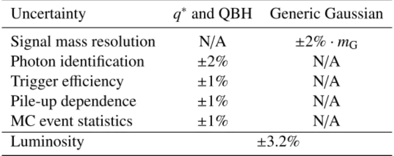
Table 1: Summary of systematic uncertainties in the signal event yield and shape included in the fit model. The signal mass resolution uncertainty affects the generic Gaussian signal shape, while the other uncertainties affect the event yield.

Uncertainty q∗and QBH Generic Gaussian

Signal mass resolution N/A ±2% · mG

Photon identification ±2% N/A

Trigger efficiency ±1% N/A

Pile-up dependence ±1% N/A

MC event statistics ±1% N/A

Luminosity ±3.2%

In order to facilitate the re-interpretation of the present results in alternative physics models, the fidu-cial acceptance and efficiency for events with the invariant mass of the γ + jet system around mq∗ or

Mth (referred to as “on-shell” events hereafter) are also provided. The chosen mγ j ranges are 0.6mq∗ <

mγ j < 1.2mq∗ for the q∗signal and 0.8M_th < m_{γ j} < 3.0M_th for the QBH signal. The fiducial region at

particle level, as summarized in Table2, is chosen to be close to the one used in the event selection at reconstruction level.

The fiducial acceptance Af, defined as the fraction of generated on-shell signal events falling into the

fiducial region, increases from 56% to 63% with increasing signal mass Mth from 1.0 to 6.5 (9.0) TeV

for the QBH in the RS1 (ADD) model. The Afvalue for the q∗model varies very similarly to that for the

RS1 QBH signal. The rise in the fiducial acceptance as a function of Mth (mq∗) is driven mainly by the

increase of the efficiency for the photon η requirement since the photons tend to be more central as Mth

(mq∗) becomes larger.

The fiducial selection efficiency εf is defined as the ratio of the number of on-shell events in the

particle-level fiducial region passing the selection at the reconstruction particle-level, including photon identification, isolation and jet quality criteria, to the number of generated on-shell events in the particle-level fiducial

Table 2: Requirements on the photon and jet at particle level to define the fiducial region and on the detector-level quantities for the selection efficiency.

Particle-level selection for fiducial region Photon : Eγ_T > 150 GeV, |ηγ|< 1.37

Jet : pjet_T > 60 GeV, |ηjet|< 4.5 Photon–Jet η separation : |∆ηγ j|< 1.6

No jet with pjet_T > 30 GeV within ∆R < 0.8 around the photon Detector-level selection for selection efficiency

Tight photon identification Photon isolation

Jet identification including quality and pile-up rejection requirements

region. The migration of generated on-shell events outside the particle-level fiducial region into the selected sample at the reconstruction level is found to be negligible. The fiducial selection efficiency decreases from 88% (86%) to 82% (80%) within the same Mthranges as above for the RS1 (ADD) QBH

model and is not highly dependent on the kinematics of the assumed signal production processes. The εffor the q∗model behaves very similarly to that for the RS1 QBH model. The reduction in the fiducial

selection efficiency is caused mainly by the inefficiency of the shower shape requirements used in the photon identification for high-ETphotons. The fiducial acceptance and selection efficiencies for the three

benchmark signal models are shown in Figure1as functions of mq∗or M_th.

) [TeV] th , M q* Signal mass (m 0 1 2 3 4 5 6 7 8 9 10 Acceptance 0.5 0.52 0.54 0.56 0.58 0.6 0.62 0.64 0.66 QBH (ADD) QBH (RS1) q* Simulation ATLAS =13 TeV s +jet γ (a) ) [TeV] th , M q* Signal mass (m 0 1 2 3 4 5 6 7 8 9 10 Efficiency 0.78 0.8 0.82 0.84 0.86 0.88 0.9 QBH (ADD) QBH (RS1) q* Simulation ATLAS =13 TeV s +jet γ (b)

Figure 1:(a)Fiducial acceptance and(b)selection efficiencies for the three signal models considered in the analysis

as a function of the excited-quark mass mq∗or the QBH threshold mass M_th. The fiducial region definition is detailed

in Table2. The description of the selection criteria can be found in the text.

5.2 Background modelling

The mγ jdistribution of the background is modelled using a functional form. A family of functions, similar to the ones used in the previous searches for γ+ jet [13,14,16] and γγ resonances [54] as well as dijet

resonances [17] is considered:

f_bg(x)= N(1 − x)pxPki=0ai(log x)i, ₍₁₎

where x is defined as mγ j/√s, p and aiare free parameters, and N is a normalization factor. The number

of free parameters describing the normalized mass distribution is thus k+ 2 with a fixed N, where k is the stopping point of the summation in Eq. (1). The normalization N as well as the shape parameters p and ai are simultaneously determined by the final fit of the signal plus background model to data. The

goodness of a given functional form in describing the background is quantified based on the potential bias introduced in the fitted number of signal events. To quantify this bias the functional form under test is used to perform a signal+ background fit to a large sample of background events built from the Jetphox prediction. The large Jetphox event sample is used for this purpose as the shape of the background prediction can be extracted with sufficiently small statistical uncertainty.

The parton-level Jetphox calculations do not account for effects from hadronization, the underlying event and the detector resolution. Therefore, the nominal Jetphox prediction is corrected by calculating the ratio of reconstructed jet pTto parton pTin the Sherpa γ + jet sample and applying the parameterized ratio to

the Jetphox parton pT. In addition, an mγ j-dependent correction is applied to the Jetphox prediction to

account for the contribution from multijet events where one of the jets is misidentified as a photon (fake photon events). This correction is estimated from data as the inverse of the purity, defined as the fraction of real γ+jet events in the selected sample. The purity is measured in bins of mγ jby exploiting the difference

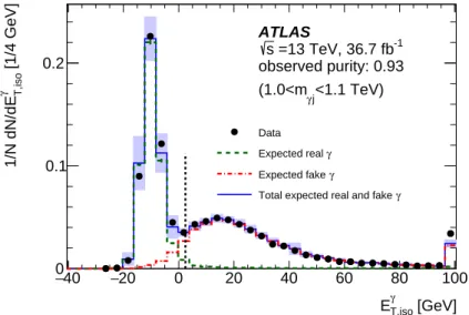
between the shapes of the Eγ_{T, iso}distributions of real photons and jets faking photons; the latter typically have a large E_{T, iso}γ value due to nearby particles produced in the jet fragmentation. The purity is estimated by performing a two-component template fit to the Eγ_{T, iso} distribution in bins of mγ j. The templates of real- and fake-photon isolation distributions are obtained from MC (Sherpa) simulation and from data control samples, respectively. The Eγ_{T, iso} variable for real photons from Sherpa simulation is corrected to account for the observed mis-modelling in the description of isolation profiles between data and MC events in a separate control sample. The template for fake photons is derived in a data sample where the photon candidate fails to satisfy the tight identification criteria but fulfils a looser set of identification criteria. Details about the correction to the real-photon template and the derivation of the fake-photon template are given in Ref. [55]. To reduce the bias in the Eγ_{T, iso} shape due to different kinematics, both the real- and fake-photon templates are obtained by applying the same set of kinematic requirements used in the main analysis. As an example, Figure2 shows the Eγ_{T, iso} distribution of events within the range 1.0 < mγ j < 1.1 TeV, superimposed on the best-fit result. This procedure is repeated in every bin of the

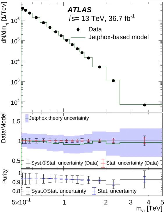
mγ j distribution and the resulting estimate of the purity is shown as a function of mγ j in Figure 3. The uncertainty in the measured purity includes both the statistical and systematic uncertainties. The latter are estimated by recomputing the purity using different data control samples for the fake-photon template or alternative templates for real photons obtained from Pythia simulation or removing the data-to-MC corrections applied to Eγ_{T, iso}in the Sherpa sample and by symmetrizing the variations. The variation from different data control samples for the fake-photon template has the largest effect on the purity (4% at 1.0 < mγ j < 1.1 TeV). The measured purity is approximately constant at 93% over the mγ j range above 500 GeV, indicating that the fake-photon contribution does not depend significantly on mγ j. Figure3

shows the mγ jdistribution in data compared to the corrected Jetphox γ + jet prediction normalized to data in the mγ j > 500 GeV region.

Theoretical uncertainties in the Jetphox prediction are computed by considering the variations induced by ±1σ of the NNPDF 2.3 PDF uncertainties, by switching between the nominal NNPDF 2.3 and CT10

or MSTW2008 PDFs, by the variation of the value of the strong coupling constant by ±0.002 around the nominal value of 0.118 and by the variation of the renormalization, factorization and fragmentation scales between half and twice the photon transverse momentum. The differences between data and the corrected Jetphox prediction shown in Figure3are well within the uncertainties associated with the perturbative QCD prediction. [GeV] γ T,iso E 40 − −20 0 20 40 60 80 100 [1/4 GeV] γ T,iso 1/N dN/dE 0 0.1 0.2 ATLAS -1 =13 TeV, 36.7 fb s observed purity: 0.93 <1.1 TeV) j γ (1.0<m Data γ Expected real γ Expected fake γ

Total expected real and fake

Figure 2: Distribution of Eγ_{T, iso}= ET, iso− 0.022 × Eγ_Tfor the photon candidates in events with 1.0 < mγ j< 1.1 TeV,

and the comparison with the result of the template fits. Real- and fake-photon components determined by the fit are shown by the green dashed and red dot-dashed histograms, respectively, and the sum of the two components is shown as the solid blue histogram. The blue band shows the systematic uncertainties in the real- plus fake-photon template. The last bin of the distribution includes overflow events. The vertical dashed line corresponds to the isolation requirement used in the analysis. The photon purity determined from the fit for the selected sample in the 1.0 < mγ j< 1.1 TeV mass range is 93%.

The number of signal events extracted by the signal + background fit to the pure background model described above is called the spurious signal [56] and it is used to select the optimal functional form and the mγ j range of the fit. In order to account for the assumption that the corrected Jetphox prediction

itself is a good representation of the data, the fit is repeated on modified samples obtained by changing the nominal shape to account for several effects: firstly, the nominal distribution is corrected to follow the envelope of the changes induced by ±1σ variations of the NNPDF 2.3 PDF uncertainty, the variations between the nominal NNPDF 2.3 and CT10 or MSTW2008 PDFs, the variation of the value of the strong coupling constant by ±0.002 around the nominal value of 0.118 and the variation of the renormalization, factorization and fragmentation scales between half and twice the photon transverse momentum; secondly the corrections for the hadronization, underlying event and detector effects are removed; and finally the corrections for the photon purity are changed within their estimated uncertainty. The largest absolute fitted signal from all variations of the nominal background sample discussed above is taken to be the spurious signal.

The spurious signal is evaluated at a number of hypothetical masses over a large search range. It is required to be less than 40% of the background’s statistical uncertainty, as quantified by the statistical uncertainty of the fitted spurious signal, anywhere in the investigated search range. In this way the impact of the systematic uncertainties due to background modelling on the analysis sensitivity is expected to be subdominant with respect to the statistical uncertainty. Functional forms that cannot meet this requirement

[1/TeV]

dN/dm

10

10

10

10

10

Data

Jetphox-based model

ATLAS

= 13 TeV, 36.7 fb

s

Data/Model

0.5

1

1.5

Stat. uncertainty (Data)

⊕

Syst. Stat. uncertainty (Data)

[TeV]

m

10

×

5

1

2

3

4

5

Purity

0.8

0.9

1

Stat. uncertainty

⊕

Syst.

Stat. uncertainty

Figure 3: Distribution of the invariant mass of the γ+ jet system as measured in the γ + jet data (dots), compared

with the Jetphox (green histogram) γ + jet predictions. The Jetphox distribution is obtained after correcting the

parton-level spectrum for showering, hadronization and detector resolution effects as described in the text. The

distributions are divided by the bin width and the Jetphox spectrum is normalized to the data in the mγ jrange above

500 GeV. The ratio of the data to Jetphox prediction as a function of mγ j is shown in the middle panel (green

histogram): the theoretical uncertainty is shown as a shaded band. The statistical uncertainty from the data sample and the sum of the statistical uncertainty plus the systematic uncertainty from the background subtraction are shown

as inner and outer bars respectively. The measured γ+ jet purity as a function of mγ jis presented in the bottom

panel (black histogram): the statistical uncertainty of the purity measurement is reported as the inner error bar while the total uncertainty is shown as the outer error bar.

are rejected. For different signal models, the functional form and fit range are determined separately. All considered functions with k up to two (four parameters) are found to fulfil the spurious-signal requirement when fitting in the range 1.1 < mγ j< 6.0 TeV for the q∗signal and 1.5 (2.5) < mγ j < 6.0 (8.0) TeV for the

RS1 (ADD) QBH signal. To further consolidate the choice of nominal background functional form, an F-test [57] is performed to determine if the change in the χ2value obtained by fitting the Jetphox sample with an additional parameter is significant. The test indicates that the k= 0 (1) functional form with two (three) parameters can describe the present data sufficiently well over the entire fit range for the QBH (q∗) signal search, and there is no improvement by adding more parameters to the background fit function. Given the fit range determined by the spurious signal test, the search is performed for the q∗(RS1 and ADD QBH) signal within the mγ j range above 1.5 (2.0 and 3.0) TeV, to account for the width of the ex-pected signal. The estimated spurious signal for the selected functional form is converted into a spurious-signal cross-section (σspur), which is included as the uncertainty due to background modelling in the

statistical analysis. The spurious-signal cross-section, and the ratio of the spurious-signal cross-section to its uncertainty (δσspur) and to the signal cross-section (σmodel) for the three benchmark models under

in-vestigation are given in Table3in the different search ranges. While both σspurand σspur/δσspurdecrease

with the hypothesized signal mass, the ratio σspur/σmodelincreases with mq∗or M_th, becoming as large as

15% in the case of excited quarks with mq∗ = 6 TeV.

Table 3: Spurious-signal cross-sections (σspur), and the ratio of the spurious-signal cross-sections to their

uncertain-ties (δσspur) and to the signal cross-sections (σmodel) for the three benchmark models. The values of these quantities

are given at the boundaries of the search range reported in the first row.

q∗ RS1 QBH ADD QBH

Search boundaries [TeV] 1.5 6.0 2.0 6.0 3.0 8.0

σspur[fb] 3.9 1.1 × 10−2 4.0 6.6 × 10−4 8.7 × 10−2 5.0 × 10−5

σspur/ δσspur[%] 37 14 39 8 20 3

σspur/σmodel[%] 0.16 15 1.0 7.5 0.0017 0.037

A similar test is performed to determine the functional form and fit ranges for the Gaussian-shaped signal with a 15% width. The test indicates that the same functional form and fit range as those used for the q∗ signal are optimal for a wide-width Gaussian signal. The same functional form and mass range is used for all the Gaussian signals.

5.3 Statistical tests

A profile-likelihood-ratio test statistic is used to quantify the compatibility of the data and the SM back-ground prediction, and to set limits on the presence of possible signal contributions in the mγ jdistribution. The likelihood function L is built from a Poisson probability for the numbers of observed events, n, and expected events, N, in the selected sample:

L= Pois(n|N(θ)) ×        n Y i=1 f(mi_{γ j}, θ)       × G(θ),

where N(θ) is the expected number of candidates, f (mi_{γ j}, θ) is the value of the probability density function of the invariant mass distribution evaluated for each candidate event i and θ are nuisance parameters. The G(θ) term collects the set of constraints on the nuisance parameters associated with the systematic

uncertainties in the signal yield, in the spurious signal and in the resolution (only for Gaussian signals) and it is represented by normal distributions centred at zero and with unit variance.

The pdf of the mγ jdistribution is given as the normalized sum of the signal and background pdfs: f(mi_{γ j}, θ) = 1

N[Nsig(θyield) fsig(m

i

γ j)+ Nbgfbg(miγ j, θbkg)],

where fsig and fbgare the normalized signal and background mγ j distributions described in the previous

sections. The θyieldare nuisance parameters associated with the signal yield uncertainties (constrained)

while θbkgare the nuisance parameters of the background shape (unconstrained). The expected number

of events N is given by the sum of the expected numbers of signal events (Nsig) and background events

(Nbg). The Nsigterm can be expressed as

Nsig(θyield)= N_sigmodel+ N_sigspur= (σmodel· B · A ·ε · F(δε, θε)+ σspur·θspur) × Lint× F(δL, θL),

where σspurand θspurare the spurious-signal cross-section described in Section5.2and its nuisance

para-meter while Lintand F(δL, θL) are the integrated luminosity and its uncertainty. Apart from the spurious

signal, systematic uncertainties with an estimated size δX are incorporated into the likelihood by

mul-tiplying the relevant parameter of the statistical model by a factor F(δX, θX) = eδXθX. The parameter of

interest in the fit to Gaussian-shaped resonances is the visible cross-section σmodel· B · A ·ε while that in

the fit to q∗and QBH signals is σmodel· B. For the latter case, the additional nuisance parameters for the

signal efficiency uncertainties F(δε, θε) are included.

The significance of a possible deviation from the SM prediction is estimated by computing the p0value,

defined as the probability of the background-only model to produce an excess at least as large as the one observed in data. Upper limits are set at 95% confidence level (CL) with a modified frequentist CLS

method on the visible cross-section (σmodel· B · A ·ε) for the Gaussian-shaped resonances or on the signal

cross-section times branching ratio (σmodel· B) for the q∗and QBH signals by identifying the value for

which the CLS value is equal to 0.05.

6 Results

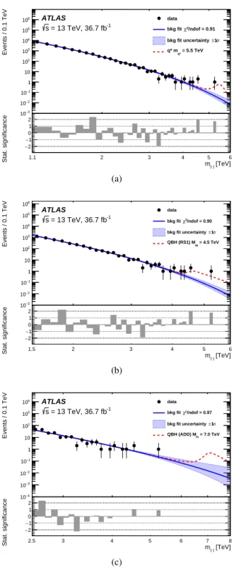
The photon–jet invariant mass distributions obtained from the selected data are shown in Figure4, to-gether with the background-only fits using the model described in Section5.2and expected distributions from the signal models under test. No significant deviation from the background prediction is observed in any of the distributions. The most significant excess is observed at 1.8 TeV with the assumption of the 2%-width Gaussian model for a local significance of 2.1 standard deviations.

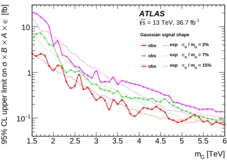
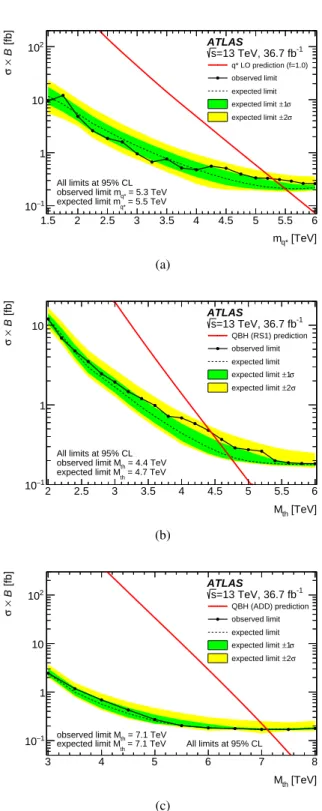
Limits are placed at 95% CL on the visible cross-section in the case of generic Gaussian-shaped reson-ances and on the production cross-section times branching ratio to a photon and a quark or gluon for the excited-quark and QBH signals. The results are shown in Figure5for the Gaussian signals with the width varying between 2% and 15%, and in Figure6for the benchmark signal models. The Gaussian signals are excluded for visible cross-sections above 0.25–1.1 fb (0.08–0.2 fb), depending on the width, at a mass m_Gof 3 TeV (5 TeV). In the case of the benchmark signal models considered in this analysis, the presence of a signal with a mass below 5.3 TeV, 4.4 TeV and 7.1 TeV for the excited quarks, RS1 and ADD QBHs, can be excluded at 95% CL. The limits improve on those in Ref. [16] by about 0.9 TeV, 0.6 TeV and 0.9 TeV for the excited quarks, RS1 and ADD QBHs, respectively.

[TeV] j γ m 2 3 4 5 6 Stat. significance 2 − 1 −0 1 2 1.1 Events / 0.1 TeV 3 − 10 2 − 10 1 − 10 1 10 2 10 3 10 4 10 5 10 6 10 ATLAS -1 = 13 TeV, 36.7 fb s data /ndof = 0.91 2 χ bkg fit σ 1 ± bkg fit uncertainty = 5.5 TeV q* q* m (a) [TeV] j γ m 2 3 4 5 6 Stat. significance 2 −−1 0 1 2 1.5 Events / 0.1 TeV 3 − 10 2 − 10 1 − 10 1 10 2 10 3 10 4 10 5 10 6 10 ATLAS -1 = 13 TeV, 36.7 fb s data /ndof = 0.90 2 χ bkg fit σ 1 ± bkg fit uncertainty = 4.5 TeV th QBH (RS1) M (b) [TeV] j γ m 3 4 5 6 7 8 Stat. significance 2 − 1 −0 1 2 2.5 Events / 0.1 TeV 4 − 10 3 − 10 2 − 10 1 − 10 1 10 2 10 3 10 4 10 ATLAS -1 = 13 TeV, 36.7 fb s data /ndof = 0.97 2 χ bkg fit σ 1 ± bkg fit uncertainty = 7.0 TeV th QBH (ADD) M (c)

Figure 4: Distributions of the invariant mass of the γ+ jet system of the observed events (dots) in 36.7 fb−1of data

at√s= 13 TeV and fits to the data (solid lines) under the background-only hypothesis for searches in the(a)excited

quarks,(b)QBH (RS1) with n= 1 and(c)QBH (ADD) with n= 6 models. The ±1σ uncertainty in the background

prediction originating from the uncertainties in the fit function parameter values is shown as a shaded band around

the fit. The predicted signal distributions (dashed lines) for the q∗model with mq∗= 5.5 TeV and the QBH model

with Mth= 4.5 (7.0) TeV based on RS1 (ADD) are shown on top of the background predictions. The bottom panels

[TeV] G m 1.5 2 2.5 3 3.5 4 4.5 5 5.5 6 [fb] ∈ × A × B × σ 95% CL upper limit on 1 − 10 1 10

Gaussian signal shape

obs = 2% G / m G σ exp obs = 7% G / m G σ exp obs = 15% G / m G σ exp ATLAS -1 = 13 TeV, 36.7 fb s

Figure 5: Observed (solid lines) and expected (dotted lines) 95% CL upper limits on the visible cross-sections σ · B · A · ε in 36.7 fb−1

of data at √s= 13 TeV as a function of the mass mGof the Gaussian resonances with three

different Gaussian widths between 2% and 15%. The calculation is performed using ensemble tests at mass points

[TeV] q* m 1.5 2 2.5 3 3.5 4 4.5 5 5.5 6 [fb] B × σ 1 − 10 1 10 2 10 ATLAS -1 =13 TeV, 36.7 fb s q* LO prediction (f=1.0) observed limit expected limit σ 1 ± expected limit σ 2 ± expected limit = 5.3 TeV q* observed limit m = 5.5 TeV q* expected limit m All limits at 95% CL (a) [TeV] th M 2 2.5 3 3.5 4 4.5 5 5.5 6 [fb] B × σ 1 − 10 1 10 ATLAS -1 =13 TeV, 36.7 fb s QBH (RS1) prediction observed limit expected limit σ 1 ± expected limit σ 2 ± expected limit = 4.4 TeV th observed limit M = 4.7 TeV th expected limit M All limits at 95% CL (b) [TeV] th M 3 4 5 6 7 8 [fb] B × σ 1 − 10 1 10 2 10 ATLAS -1 =13 TeV, 36.7 fb s QBH (ADD) prediction observed limit expected limit σ 1 ± expected limit σ 2 ± expected limit = 7.1 TeV th observed limit M = 7.1 TeV th

expected limit M All limits at 95% CL

(c)

Figure 6: Observed 95% CL upper limits (solid line with dots) on the production cross-section times branching ratio

σ· B to a photon and a quark or gluon in 36.7 fb−1_{of data at} √_{s= 13 TeV for the(a)excited-quarks,(b)QBH (RS1)}

with n= 1 and(c)QBH (ADD) with n= 6 models. The limits are placed as a function of mq∗for the excited quarks

and Mthfor the QBH signals. The calculation is performed using ensemble tests at mass points separated by 200

(500) GeV for the RS1 (ADD) model over the search range. For the q∗_{model the step size is 250 GeV up to 5 TeV}

and then 200 GeV up to 6 TeV. The limits expected if a signal is absent (dashed lines) are shown together with the ±1σ and ±2σ intervals represented by the green and yellow bands, respectively. The theoretical predictions of σ · B for the respective benchmark signals are shown by the red solid lines.

7 Conclusion

A search is performed for new phenomena in events having a photon with high transverse momentum and a jet collected in 36.7 fb−1of pp collision data at a centre-of-mass energy of √s= 13 TeV recorded with the ATLAS detector at the LHC. The invariant mass distribution of the γ+ jet system above 1.1 TeV is used in the search for localized excesses of events. No significant deviation is found. Limits are set on the visible cross-section for generic Gaussian-shaped resonances and on the production cross-section times branching ratio for signals predicted in models of excited quarks or quantum black holes. The data exclude, at 95% CL, the mass range below 5.3 TeV for the excited quarks and 7.1 (4.4) TeV for the quantum black holes with six (one) extra dimensions in the Arkani-Hamed–Dimopoulos–Dvali (Randall– Sundrum) model. These limits supersede the previous ATLAS exclusion limits for excited quarks and quantum black holes in the γ+ jet final state.

Acknowledgements

We thank CERN for the very successful operation of the LHC, as well as the support staff from our institutions without whom ATLAS could not be operated efficiently.

We acknowledge the support of ANPCyT, Argentina; YerPhI, Armenia; ARC, Australia; BMWFW and FWF, Austria; ANAS, Azerbaijan; SSTC, Belarus; CNPq and FAPESP, Brazil; NSERC, NRC and CFI, Canada; CERN; CONICYT, Chile; CAS, MOST and NSFC, China; COLCIENCIAS, Colombia; MSMT CR, MPO CR and VSC CR, Czech Republic; DNRF and DNSRC, Denmark; IN2P3-CNRS, CEA-DSM/IRFU, France; SRNSF, Georgia; BMBF, HGF, and MPG, Germany; GSRT, Greece; RGC, Hong Kong SAR, China; ISF, I-CORE and Benoziyo Center, Israel; INFN, Italy; MEXT and JSPS, Ja-pan; CNRST, Morocco; NWO, Netherlands; RCN, Norway; MNiSW and NCN, Poland; FCT, Portugal; MNE/IFA, Romania; MES of Russia and NRC KI, Russian Federation; JINR; MESTD, Serbia; MSSR, Slovakia; ARRS and MIZŠ, Slovenia; DST/NRF, South Africa; MINECO, Spain; SRC and Wallen-berg Foundation, Sweden; SERI, SNSF and Cantons of Bern and Geneva, Switzerland; MOST, Taiwan; TAEK, Turkey; STFC, United Kingdom; DOE and NSF, United States of America. In addition, indi-vidual groups and members have received support from BCKDF, the Canada Council, CANARIE, CRC, Compute Canada, FQRNT, and the Ontario Innovation Trust, Canada; EPLANET, ERC, ERDF, FP7, Horizon 2020 and Marie Skłodowska-Curie Actions, European Union; Investissements d’Avenir Labex and Idex, ANR, Région Auvergne and Fondation Partager le Savoir, France; DFG and AvH Foundation, Germany; Herakleitos, Thales and Aristeia programmes co-financed by EU-ESF and the Greek NSRF; BSF, GIF and Minerva, Israel; BRF, Norway; CERCA Programme Generalitat de Catalunya, Generalitat Valenciana, Spain; the Royal Society and Leverhulme Trust, United Kingdom.

The crucial computing support from all WLCG partners is acknowledged gratefully, in particular from CERN, the ATLAS Tier-1 facilities at TRIUMF (Canada), NDGF (Denmark, Norway, Sweden), CC-IN2P3 (France), KIT/GridKA (Germany), INFN-CNAF (Italy), NL-T1 (Netherlands), PIC (Spain), ASGC (Taiwan), RAL (UK) and BNL (USA), the Tier-2 facilities worldwide and large non-WLCG resource pro-viders. Major contributors of computing resources are listed in Ref. [58].

References

[1] U. Baur, I. Hinchliffe and D. Zeppenfeld, Excited Quark Production at Hadron Colliders,

Int. J. Mod. Phys. A 2 (1987) 1285.

[2] U. Baur, M. Spira and P. M. Zerwas, Excited-quark and -lepton production at hadron colliders,

Phys. Rev. D 42 (1990) 815.

[3] S. Bhattacharya, S. S. Chauhan, B. C. Choudhary and D. Choudhury, Quark excitations through the prism of direct photon plus jet at the LHC,

Phys. Rev. D 80 (2009) 015014, arXiv:0901.3927 [hep-ph]. [4] S. Weinberg, Gauge Hierarchies,Phys. Lett. B 82 (1979) 387.

[5] M. J. G. Veltman, The Infrared - Ultraviolet Connection, Acta Phys. Polon. B 12 (1981) 437. [6] C.H. Llewellyn Smith, G. G. Ross, The Real Gauge Hierarchy Problem,

Phys. Lett. B 105 (1981) 38.

[7] S. Dimopoulos and G. L. Landsberg, Black holes at the Large Hadron Collider,

Phys. Rev. Lett. 87 (2001) 161602, arXiv:hep-ph/0106295. [8] S. B. Giddings and S. D. Thomas,

High energy colliders as black hole factories: The end of short distance physics,

Phys. Rev. D 65 (2002) 056010, arXiv:hep-ph/0106219.

[9] D. M. Gingrich, Quantum black holes with charge, colour, and spin at the LHC,

J. Phys. G 37 (2010) 105008, arXiv:0912.0826 [hep-ph].

[10] X. Calmet, W. Gong and S. D. Hsu, Colorful quantum black holes at the LHC,

Phys. Lett. B 668 (2008) 20, arXiv:0806.4605 [hep-ph]. [11] N. Arkani-Hamed, S. Dimopoulos and G. Dvali,

The Hierarchy problem and new dimensions at a millimeter,Phys. Lett. B 429 (1998) 263, arXiv:hep-ph/9803315.

[12] L. Randall and R. Sundrum, A Large mass hierarchy from a small extra dimension,

Phys. Rev. Lett. 83 (1999) 3370, arXiv:hep-ph/9905221.

[13] ATLAS Collaboration, Search for Production of Resonant States in the Photon-Jet Mass Distribution Using pp Collisions at at √s= 7 TeV Collected by the ATLAS Detector,

Phys. Rev. Lett. 108 (2012) 211802, arXiv:1112.3580 [hep-ex].

[14] ATLAS Collaboration, Search for new phenomena in photon+jet events collected in

proton–proton collisions at √s= 8 TeV with the ATLAS detector,Phys. Lett. B 728 (2014) 562, arXiv:1309.3230 [hep-ex].

[15] CMS Collaboration,

Search for excited quarks in theγ+jet final state in proton–proton collisions at √s= 8 TeV,

Phys. Lett. B 738 (2014) 274, arXiv:1406.5171 [hep-ex].

[16] ATLAS Collaboration, Search for new phenomena with photon+jet events in proton–proton collisions at √s= 13 TeV with the ATLAS detector,JHEP 03 (2016) 041,

arXiv:1512.05910 [hep-ex].

[17] ATLAS Collaboration, Search for New Phenomena in Dijet Mass and Angular Distributions from pp Collisions at √s= 13 TeV with the ATLAS Detector,Phys. Lett. B 754 (2016) 302,

[18] ATLAS Collaboration, Search for new phenomena in dijet events using 37 fb−1of pp collision data collected at √s= 13 TeV with the ATLAS detector, (2017), arXiv:1703.09127 [hep-ex]. [19] CMS Collaboration, Search for dijet resonances in proton–proton collisions at √s= 13 TeV and

constraints on dark matter and other models,Phys. Lett. B 769 (2017) 520, arXiv:1611.03568 [hep-ex].

[20] ATLAS Collaboration, The ATLAS Experiment at the CERN Large Hadron Collider,

JINST 3 (2008) S08003.

[21] ATLAS Collaboration, ATLAS Insertable B-Layer Technical Design Report, ATLAS-TDR-19, 2010, url:https://cds.cern.ch/record/1291633,

ATLAS Insertable B-Layer Technical Design Report Addendum, ATLAS-TDR-19-ADD-1, 2012,

URL:https://cds.cern.ch/record/1451888.

[22] ATLAS Collaboration, Performance of the ATLAS Trigger System in 2015,

Eur. Phys. J. C 77 (2017) 317, arXiv:1611.09661 [hep-ex]. [23] ATLAS Collaboration,

Luminosity determination in pp collisions at √s= 8 TeV using the ATLAS detector at the LHC,

Eur. Phys. J. C 76 (2016) 653, arXiv:1608.03953 [hep-ex]. [24] T. Gleisberg, S. Höche, F. Krauss, M. Schönherr, S. Schumann et al.,

Event generation with SHERPA 1.1,JHEP 02 (2009) 007, arXiv:0811.4622 [hep-ph]. [25] S. Schumann and F. Krauss,

A Parton shower algorithm based on Catani-Seymour dipole factorisation,JHEP 03 (2008) 038, arXiv:0709.1027 [hep-ph].

[26] S. Höche, F. Krauss, S. Schumann and F. Siegert, QCD matrix elements and truncated showers,

JHEP 05 (2009) 053, arXiv:0903.1219 [hep-ph].

[27] H.-L. Lai et al., New parton distributions for collider physics,Phys. Rev. D 82 (2010) 074024, arXiv:1007.2241 [hep-ph].

[28] T. Sjöstrand et al., An introduction to PYTHIA 8.2,Comput. Phys. Commun. 191 (2015) 159, arXiv:1410.3012 [hep-ph].

[29] ATLAS Collaboration, ATLAS Pythia 8 tunes to 7 TeV data, ATL-PHYS-PUB-2014-021, 2014,

url:https://cds.cern.ch/record/1966419.

[30] S. Catani, M. Fontannaz, J. P. Guillet and E. Pilon,

Cross-section of isolated prompt photons in hadron hadron collisions,JHEP 05 (2002) 028, arXiv:hep-ph/0204023.

[31] L. Bourhis, M. Fontannaz, J. Guillet and M. Werlen,

Next-to-leading order determination of fragmentation functions,Eur. Phys. J. C 19 (2001) 89, arXiv:hep-ph/0009101.

[32] R. D. Ball et al., Parton distributions with LHC data,Nucl. Phys. B 867 (2013) 244, arXiv:1207.1303 [hep-ph].

[33] M. Cacciari, G. P. Salam and G. Soyez, The anti-ktjet clustering algorithm,JHEP 04 (2008) 063,

arXiv:0802.1189 [hep-ph].

[34] M. Cacciari, G. P. Salam and G. Soyez, FastJet User Manual,Eur. Phys. J. C 72 (2012) 1896, arXiv:1111.6097 [hep-ph].

[35] D. M. Gingrich,

Monte Carlo event generator for black hole production and decay in proton-proton collisions,

Comput. Phys. Commun. 181 (2010) 1917, arXiv:0911.5370 [hep-ph]. [36] J. Pumplin et al.,

New generation of parton distributions with uncertainties from global QCD analysis,

JHEP 07 (2002) 012, arXiv:hep-ph/0201195.

[37] ATLAS Collaboration, The ATLAS Simulation Infrastructure,Eur. Phys. J. C 70 (2010) 823, arXiv:1005.4568 [hep-ex].

[38] S. Agostinelli et al., GEANT4–a simulation toolkit,Nucl. Instrum. Meth. A 506 (2003) 250. [39] ATLAS Collaboration, Summary of ATLAS Pythia 8 tunes, ATL-PHYS-PUB-2012-003, 2012,

url:https://cds.cern.ch/record/1474107.

[40] A. D. Martin, W. J. Stirling, R. S. Thorne and G. Watt, Parton distributions for the LHC,

Eur. Phys. J. C 63 (2009) 189, arXiv:0901.0002 [hep-ph].

[41] ATLAS Collaboration, Measurement of the photon identification efficiencies with the ATLAS detector using LHC Run-1 data,Eur. Phys. J. C 76 (2016) 666, arXiv:1606.01813 [hep-ex]. [42] ATLAS Collaboration,

Electron and photon energy calibration with the ATLAS detector using LHC Run 1 data,

Eur. Phys. J. C 74 (2014) 3071, arXiv:1407.5063 [hep-ex]. [43] ATLAS Collaboration,

Topological cell clustering in the ATLAS calorimeters and its performance in LHC Run 1,

Eur. Phys. J. C 77 (2017) 490, arXiv:1603.02934 [hep-ex].

[44] ATLAS Collaboration, Measurement of the inclusive isolated prompt photon cross section in pp collisions at √s= 7 TeV with the ATLAS detector,Phys. Rev. D 83 (2011) 052005,

arXiv:1012.4389 [hep-ex].

[45] ATLAS Collaboration, Performance of pile-up mitigation techniques for jets in pp collisions at_√ s= 8 TeV using the ATLAS detector,Eur. Phys. J. C 76 (2016) 581,

arXiv:1510.03823 [hep-ex].

[46] ATLAS Collaboration, Jet energy scale measurements and their systematic uncertainties in proton–proton collisions at √s= 13 TeV with the ATLAS detector, (2017),

arXiv:1703.09665 [hep-ex].

[47] ATLAS Collaboration, Jet global sequential corrections with the ATLAS detector in proton–proton collisions at √s= 8 TeV, ATLAS-CONF-2015-002, 2015,

url:https://cds.cern.ch/record/2001682.

[48] ATLAS Collaboration, Tagging and suppression of pileup jets with the ATLAS detector, ATLAS-CONF-2014-018, 2014, url:https://cds.cern.ch/record/1700870. [49] ATLAS Collaboration,

Selection of jets produced in13 TeV proton–proton collisions with the ATLAS detector, ATLAS-CONF-2015-029, 2015, url:https://cds.cern.ch/record/2037702. [50] G. Cowan, K. Cranmer, E. Gross and O. Vitells,

Asymptotic formulae for likelihood-based tests of new physics,Eur. Phys. J. C 71 (2011) 1554, arXiv:1007.1727 [physics.data-an], Erratum:Eur. Phys. J. C 73 (2013) 2501.

[52] K. S. Cranmer, Kernel estimation in high-energy physics,

Comput. Phys. Commun. 136 (2001) 198, arXiv:hep-ex/0011057.

[53] M. Baak, S. Gadatsch, R. Harrington and W. Verkerke, Interpolation between multi-dimensional histograms using a new non-linear moment morphing method,

Nucl. Instrum. Meth. A 771 (2015) 39, arXiv:1410.7388 [physics.data-an]. [54] ATLAS Collaboration,

Search for resonances in diphoton events at √s=13 TeV with the ATLAS detector,

JHEP 09 (2016) 001, arXiv:1606.03833 [hep-ex].

[55] ATLAS Collaboration, High-E_√ T isolated-photon plus jets production in pp collisions at

s= 8 TeV with the ATLAS detector,Nucl. Phys. B 918 (2017) 257, arXiv:1611.06586 [hep-ex].

[56] ATLAS Collaboration, Observation of a new particle in the search for the Standard Model Higgs boson with the ATLAS detector at the LHC,Phys. Lett. B 716 (2012) 1,

arXiv:1207.7214 [hep-ex].

[57] R. A. Fisher, On the Interpretation of χ2from Contingency Tables, and the Calculation of P,

J. Royal Statistical Society 85 (1922) 87.

[58] ATLAS Collaboration, ATLAS Computing Acknowledgements 2016–2017,

The ATLAS Collaboration

M. Aaboud137d, G. Aad88, B. Abbott115, O. Abdinov12,∗, B. Abeloos119, S.H. Abidi161,

O.S. AbouZeid139, N.L. Abraham151, H. Abramowicz155, H. Abreu154, R. Abreu118, Y. Abulaiti148a,148b, B.S. Acharya167a,167b,a, S. Adachi157, L. Adamczyk41a, J. Adelman110, M. Adersberger102, T. Adye133, A.A. Affolder139_{, Y. Afik}154_{, T. Agatonovic-Jovin}14_{, C. Agheorghiesei}28c_{, J.A. Aguilar-Saavedra}128a,128f_,

S.P. Ahlen24, F. Ahmadov68,b, G. Aielli135a,135b, S. Akatsuka71, H. Akerstedt148a,148b, T.P.A. Åkesson84, E. Akilli52, A.V. Akimov98, G.L. Alberghi22a,22b, J. Albert172, P. Albicocco50, M.J. Alconada Verzini74, S.C. Alderweireldt108, M. Aleksa32, I.N. Aleksandrov68, C. Alexa28b, G. Alexander155,

T. Alexopoulos10, M. Alhroob115, B. Ali130, M. Aliev76a,76b, G. Alimonti94a, J. Alison33, S.P. Alkire38, B.M.M. Allbrooke151_{, B.W. Allen}118_{, P.P. Allport}19_{, A. Aloisio}106a,106b_{, A. Alonso}39_{, F. Alonso}74_,

C. Alpigiani140, A.A. Alshehri56, M.I. Alstaty88, B. Alvarez Gonzalez32, D. Álvarez Piqueras170, M.G. Alviggi106a,106b, B.T. Amadio16, Y. Amaral Coutinho26a, C. Amelung25, D. Amidei92, S.P. Amor Dos Santos128a,128c_{, S. Amoroso}32_{, G. Amundsen}25_{, C. Anastopoulos}141_{, L.S. Ancu}52_,

N. Andari19, T. Andeen11, C.F. Anders60b, J.K. Anders77, K.J. Anderson33, A. Andreazza94a,94b, V. Andrei60a, S. Angelidakis37, I. Angelozzi109, A. Angerami38, A.V. Anisenkov111,c, N. Anjos13, A. Annovi126a,126b, C. Antel60a, M. Antonelli50, A. Antonov100,∗, D.J. Antrim166, F. Anulli134a, M. Aoki69, L. Aperio Bella32, G. Arabidze93, Y. Arai69, J.P. Araque128a, V. Araujo Ferraz26a, A.T.H. Arce48, R.E. Ardell80, F.A. Arduh74, J-F. Arguin97, S. Argyropoulos66, M. Arik20a, A.J. Armbruster32, L.J. Armitage79, O. Arnaez161, H. Arnold51, M. Arratia30, O. Arslan23,

A. Artamonov99,∗, G. Artoni122, S. Artz86, S. Asai157, N. Asbah45, A. Ashkenazi155, L. Asquith151, K. Assamagan27, R. Astalos146a, M. Atkinson169, N.B. Atlay143, K. Augsten130, G. Avolio32, B. Axen16, M.K. Ayoub35a, G. Azuelos97,d, A.E. Baas60a, M.J. Baca19, H. Bachacou138, K. Bachas76a,76b,

M. Backes122, P. Bagnaia134a,134b, M. Bahmani42, H. Bahrasemani144, J.T. Baines133, M. Bajic39, O.K. Baker179, P.J. Bakker109, E.M. Baldin111,c, P. Balek175, F. Balli138, W.K. Balunas124, E. Banas42, A. Bandyopadhyay23, Sw. Banerjee176,e, A.A.E. Bannoura178, L. Barak155, E.L. Barberio91,

D. Barberis53a,53b, M. Barbero88, T. Barillari103, M-S Barisits32, J.T. Barkeloo118, T. Barklow145, N. Barlow30, S.L. Barnes36c, B.M. Barnett133, R.M. Barnett16, Z. Barnovska-Blenessy36a, A. Baroncelli136a, G. Barone25, A.J. Barr122, L. Barranco Navarro170, F. Barreiro85,

J. Barreiro Guimarães da Costa35a, R. Bartoldus145, A.E. Barton75, P. Bartos146a, A. Basalaev125, A. Bassalat119, f, R.L. Bates56, S.J. Batista161, J.R. Batley30, M. Battaglia139, M. Bauce134a,134b, F. Bauer138, H.S. Bawa145,g, J.B. Beacham113, M.D. Beattie75, T. Beau83, P.H. Beauchemin165, P. Bechtle23, H.P. Beck18,h, H.C. Beck57, K. Becker122, M. Becker86, C. Becot112, A.J. Beddall20e, A. Beddall20b, V.A. Bednyakov68, M. Bedognetti109, C.P. Bee150, T.A. Beermann32, M. Begalli26a, M. Begel27, J.K. Behr45, A.S. Bell81, G. Bella155, L. Bellagamba22a, A. Bellerive31, M. Bellomo154, K. Belotskiy100, O. Beltramello32, N.L. Belyaev100, O. Benary155,∗, D. Benchekroun137a, M. Bender102, N. Benekos10, Y. Benhammou155, E. Benhar Noccioli179, J. Benitez66, D.P. Benjamin48, M. Benoit52, J.R. Bensinger25, S. Bentvelsen109, L. Beresford122, M. Beretta50, D. Berge109,

E. Bergeaas Kuutmann168, N. Berger5, J. Beringer16, S. Berlendis58, N.R. Bernard89, G. Bernardi83, C. Bernius145, F.U. Bernlochner23, T. Berry80, P. Berta86, C. Bertella35a, G. Bertoli148a,148b,

I.A. Bertram75, C. Bertsche45, D. Bertsche115, G.J. Besjes39, O. Bessidskaia Bylund148a,148b,

M. Bessner45, N. Besson138, A. Bethani87, S. Bethke103, A.J. Bevan79, J. Beyer103, R.M. Bianchi127, O. Biebel102, D. Biedermann17, R. Bielski87, K. Bierwagen86, N.V. Biesuz126a,126b, M. Biglietti136a, T.R.V. Billoud97, H. Bilokon50, M. Bindi57, A. Bingul20b, C. Bini134a,134b, S. Biondi22a,22b, T. Bisanz57, C. Bittrich47, D.M. Bjergaard48, J.E. Black145, K.M. Black24, R.E. Blair6, T. Blazek146a, I. Bloch45, C. Blocker25, A. Blue56, W. Blum86,∗, U. Blumenschein79, S. Blunier34a, G.J. Bobbink109,

V.S. Bobrovnikov111,c_{, S.S. Bocchetta}84_{, A. Bocci}48_{, C. Bock}102_{, M. Boehler}51_{, D. Boerner}178_,

D. Bogavac102, A.G. Bogdanchikov111, C. Bohm148a, V. Boisvert80, P. Bokan168,i, T. Bold41a, A.S. Boldyrev101, A.E. Bolz60b, M. Bomben83, M. Bona79, M. Boonekamp138, A. Borisov132,

G. Borissov75, J. Bortfeldt32, D. Bortoletto122, V. Bortolotto62a,62b,62c, D. Boscherini22a, M. Bosman13, J.D. Bossio Sola29, J. Boudreau127, J. Bouffard2, E.V. Bouhova-Thacker75, D. Boumediene37,

C. Bourdarios119, S.K. Boutle56, A. Boveia113, J. Boyd32, I.R. Boyko68, A.J. Bozson80, J. Bracinik19, A. Brandt8, G. Brandt57, O. Brandt60a, F. Braren45, U. Bratzler158, B. Brau89, J.E. Brau118,

W.D. Breaden Madden56, K. Brendlinger45, A.J. Brennan91, L. Brenner109, R. Brenner168,

S. Bressler175, D.L. Briglin19, T.M. Bristow49, D. Britton56, D. Britzger45, F.M. Brochu30, I. Brock23, R. Brock93, G. Brooijmans38, T. Brooks80, W.K. Brooks34b, J. Brosamer16, E. Brost110,

J.H Broughton19, P.A. Bruckman de Renstrom42, D. Bruncko146b, A. Bruni22a, G. Bruni22a, L.S. Bruni109, S. Bruno135a,135b, BH Brunt30, M. Bruschi22a, N. Bruscino127, P. Bryant33, L. Bryngemark45, T. Buanes15, Q. Buat144, P. Buchholz143, A.G. Buckley56, I.A. Budagov68,

F. Buehrer51, M.K. Bugge121, O. Bulekov100, D. Bullock8, T.J. Burch110, S. Burdin77, C.D. Burgard51, A.M. Burger5, B. Burghgrave110, K. Burka42, S. Burke133, I. Burmeister46, J.T.P. Burr122, E. Busato37, D. Büscher51, V. Büscher86, P. Bussey56, J.M. Butler24, C.M. Buttar56, J.M. Butterworth81, P. Butti32, W. Buttinger27, A. Buzatu153, A.R. Buzykaev111,c, S. Cabrera Urbán170, D. Caforio130, H. Cai169, V.M. Cairo40a,40b, O. Cakir4a, N. Calace52, P. Calafiura16, A. Calandri88, G. Calderini83, P. Calfayan64, G. Callea40a,40b, L.P. Caloba26a, S. Calvente Lopez85, D. Calvet37, S. Calvet37, T.P. Calvet88,

R. Camacho Toro33, S. Camarda32, P. Camarri135a,135b, D. Cameron121, R. Caminal Armadans169, C. Camincher58, S. Campana32, M. Campanelli81, A. Camplani94a,94b, A. Campoverde143,

V. Canale106a,106b, M. Cano Bret36c, J. Cantero116, T. Cao155, M.D.M. Capeans Garrido32, I. Caprini28b, M. Caprini28b, M. Capua40a,40b, R.M. Carbone38, R. Cardarelli135a, F. Cardillo51, I. Carli131, T. Carli32, G. Carlino106a, B.T. Carlson127, L. Carminati94a,94b, R.M.D. Carney148a,148b, S. Caron108, E. Carquin34b, S. Carrá94a,94b, G.D. Carrillo-Montoya32, D. Casadei19, M.P. Casado13, j, M. Casolino13, D.W. Casper166, R. Castelijn109, V. Castillo Gimenez170, N.F. Castro128a,k, A. Catinaccio32, J.R. Catmore121, A. Cattai32, J. Caudron23, V. Cavaliere169, E. Cavallaro13, D. Cavalli94a, M. Cavalli-Sforza13, V. Cavasinni126a,126b, E. Celebi20d, F. Ceradini136a,136b, L. Cerda Alberich170, A.S. Cerqueira26b, A. Cerri151,

L. Cerrito135a,135b, F. Cerutti16, A. Cervelli22a,22b, S.A. Cetin20d, A. Chafaq137a, D. Chakraborty110, S.K. Chan59, W.S. Chan109, Y.L. Chan62a, P. Chang169, J.D. Chapman30, D.G. Charlton19, C.C. Chau31, C.A. Chavez Barajas151, S. Che113, S. Cheatham167a,167c, A. Chegwidden93, S. Chekanov6,

S.V. Chekulaev163a, G.A. Chelkov68,l, M.A. Chelstowska32, C. Chen36a, C. Chen67, H. Chen27, J. Chen36a, S. Chen35b, S. Chen157, X. Chen35c,m, Y. Chen70, H.C. Cheng92, H.J. Cheng35a, A. Cheplakov68, E. Cheremushkina132, R. Cherkaoui El Moursli137e, E. Cheu7, K. Cheung63, L. Chevalier138_{, V. Chiarella}50_{, G. Chiarelli}126a,126b_{, G. Chiodini}76a_{, A.S. Chisholm}32_{, A. Chitan}28b_,

Y.H. Chiu172, M.V. Chizhov68, K. Choi64, A.R. Chomont37, S. Chouridou156, Y.S. Chow62a,

V. Christodoulou81, M.C. Chu62a, J. Chudoba129, A.J. Chuinard90, J.J. Chwastowski42, L. Chytka117, A.K. Ciftci4a, D. Cinca46, V. Cindro78, I.A. Cioara23, A. Ciocio16, F. Cirotto106a,106b, Z.H. Citron175, M. Citterio94a, M. Ciubancan28b, A. Clark52, B.L. Clark59, M.R. Clark38, P.J. Clark49, R.N. Clarke16, C. Clement148a,148b, Y. Coadou88, M. Cobal167a,167c, A. Coccaro52, J. Cochran67, L. Colasurdo108, B. Cole38, A.P. Colijn109, J. Collot58, T. Colombo166, P. Conde Muiño128a,128b, E. Coniavitis51, S.H. Connell147b, I.A. Connelly87, S. Constantinescu28b, G. Conti32, F. Conventi106a,n, M. Cooke16, A.M. Cooper-Sarkar122, F. Cormier171, K.J.R. Cormier161, M. Corradi134a,134b, F. Corriveau90,o,

A. Cortes-Gonzalez32, G. Costa94a, M.J. Costa170, D. Costanzo141, G. Cottin30, G. Cowan80, B.E. Cox87, K. Cranmer112, S.J. Crawley56, R.A. Creager124, G. Cree31, S. Crépé-Renaudin58, F. Crescioli83,

W.A. Cribbs148a,148b, M. Cristinziani23, V. Croft112, G. Crosetti40a,40b, A. Cueto85,