Transportation infrastructures in a low carbon world: An evaluation of investment needs and their determinants

HAL Id: hal-02131954

https://hal.archives-ouvertes.fr/hal-02131954

HAL is a multi-disciplinary open access archive for the deposit and dissemination of sci-entific research documents, whether they are pub-lished or not. The documents may come from teaching and research institutions in France or abroad, or from public or private research centers.

L’archive ouverte pluridisciplinaire HAL, est destinée au dépôt et à la diffusion de documents scientifiques de niveau recherche, publiés ou non, émanant des établissements d’enseignement et de recherche français ou étrangers, des laboratoires publics ou privés.

Transportation infrastructures in a low carbon world:

An evaluation of investment needs and their

determinants

Vivien Fisch-Romito, Céline Guivarch

To cite this version:

Vivien Fisch-Romito, Céline Guivarch. Transportation infrastructures in a low carbon world: An evaluation of investment needs and their determinants. Transportation Research Part D: Transport and Environment, Elsevier, 2019, 72, pp.203-219. �10.1016/j.trd.2019.04.014�. �hal-02131954�

1

Transportation infrastructures in a low carbon

world: an evaluation of investment needs and

their determinants

Vivien Fisch-Romito

_{and Céline Guivarch}

1_{CIRED, 45 bis avenue de la Belle Gabrielle, Nogent-sur-Marne Cedex 94736, France} 2_{École des Ponts—ParisTech, 6-8 Avenue Blaise Pascal, Cité Descartes, Champs sur}

Marne, 77455 Marne la Vallée Cedex 2, France

Abstract

Transportation infrastructures will either lock in transportation patterns in CO2 high-emitting modes or foster low-carbon pathways. At the same time, increases in future mobility demand require the rapid development of new infrastructures. Here we quantify investment needs for transportation infrastructures over time to achieve both development and climate objectives. We compared investment needs between world regions and analyzed their main determinants. To do so, we built socio-economic scenarios with the Imaclim-R integrated assessment model, combining alternatives for model parameters that determine mobility patterns. We then estimated the levels of investment that are consistent with the passenger and freight transportation trends in the different scenarios with and without climate policy. Finally, we used a global sensitivity analysis to identify the determinants of investments in low-carbon scenarios. We find that the expenditure needed for transportation infrastructure is lower in low-carbon pathways than in baseline scenarios. This result holds true at both the global and regional scales and is robust to the uncertainties considered. This o ve rall d ecrease is brought abo u t in particu lar by a red uctio n in tr anspor t activity. Rail utilization rates and road construction costs are determining factors for investment in all regions. Modal shift from road to rail can be a lever to reduce investment needs only if combined with

2

action on rail infrastructure occupancy. To obtain a comprehensive assessment of the costs related to the transport sector in a low-carbon world, additional investments not considered in this study related to energy efficiency or alternative fuels use should be integrated.

Keywords— transportation infrastructures; investment needs; low-carbon pathways; modeling

1 Introduction

Transportation is one of the fastest growing GHG emitting sectors, having undergone the highest growth in greenhouse gas emissions since 1970 (Sims et al., 2014), reaching 7.5 GtCO2

eq in 2014 (IEA, 2017a). In 2015, global transportation activity accounted for 26% of final energy use and 65% of oil consumption (IEA, 2017b). Significant reductions in emissions from the transportation sector will therefore be needed to keep global temperature rise below 2◦_C.

Transportation mode choices and the resulting emissions are influenced by transportation infrastructures. Infrastructure planning can be a lever for a shift to low-carbon modes not only in developed countries (Henao et al., 2015) but also in emerging countries (Tiwari et al., 2016). Conversely, transportation infrastructures can cause lock-in on high carbon emissions because of their very long lifespans (Guivarch & Hallegatte, 2011). Transportation infrastructure planning is therefore an essential aspect of any strategy to reduce greenhouse gas emissions.

At the same time, transportation activity will rise over the coming decades, especially in developing countries as demographic and economic growth drive increasing per capita mobility (Schäfer, 2009). In the next four decades, global passenger and freight travel is expected to double over 2010 levels (Dulac, 2013). This future increase in mobility demand requires a rapid build-up of new infrastructure and an upgrade to existing stock.

3

Latin America (Perrotti & Sánchez, 2011) or the USA (OECD, 2017) have already experienced shortfalls in this area in recent decades. The impact of climate policies on infrastructure investment is essentially ambiguous and could exacerbate the investment gap in some countries or release tension in others. With regard to rail infrastructure, for instance, investment needs would, on the one hand, be stimulated by a modal shift in freight transportation from road to rail. On the other hand, investment needs could be driven down by decreasing demand for coal transportation (Kennedy & Corfee-Morlot, 2013).

Therefore, transportation infrastructure stands at the intersection between climate and development imperatives, and the question of the investment needs for transportation infrastructure to achieve transitions to low-carbon modes while pursuing development goals worldwide is part of the broader question of the finance needed to achieve climate and sustainable development objectives. This article seeks to contribute to this discussion by quantifying the investment needed for transportation infrastructure that promotes low-carbon pathways and analyzing how it differs (or resembles) the investment needed for high-carbon pathways.

Several analyses have already been carried out on the issue of global investment in transportation infrastructure. OECD (2006) forecasted investment needs in rail and road capital stock between 2005 and 2030 using the econometric relationship between infrastructure capital stock and per capita GDP. OECD (2012) updated the figures on rail and extends the analysis to other infrastructures, such as ports and airports. Dobbs et al. (2013) estimated transportation-specific spending (road, rail, airports, and harbors) through two different approaches, respectively based on historical spending on transportation infrastructures, and on the historical value of infrastructure stock compared with GDP. However, all these studies have in common the fact that they do not take climate policies into account in their assessments and have a short time horizon compared with the timeframe for the implementation of climate policies. Dulac (2013)

4

compared the land transportation infrastructure required to support transportation activity projections built with the IEA Mobility Model (MoMo) for a baseline scenario and for a low-carbon scenario – the IEA ‘4DS’ and ‘2DS’ scenarios (IEA, 2012). IEA (2016) updated the figures with new assumptions on costs and calculations and a more fine-grained disaggregation of passenger rail infrastructure into high-speed, intercity, and metro/urban rail.

The issue of investment needs for low-carbon pathways has also been addressed using integrated assessment models (IAM), which have the advantage of taking into account the major interactions between energy, land-use, economic, and climate systems, but the assessments undertaken through this approach focus mainly on the energy sector (Bosetti et al., 2009; Carraro et al., 2012 ; Tavoni et al., 2015; ; McCollum et al., 2018). Most of the models do not take investment in transportation infrastructures into account in their global estimation of costs (Creutzig et al., 2015), although the amounts of investment involved are of the same order of magnitude or higher than total investments in the energy sector. The only contribution is from Broin & Guivarch (2017), where the authors incorporated the costs of the construction and maintenance of transportation infrastructure into an IAM and compare a baseline scenario with a low-carbon scenario. The authors showed that the investment required is lower if climate policies implemented for low, medium, and high income countries.

Few studies have focused on specific regions, such as Perrotti & Sánchez (2011) for Latin America and Bhattacharyay (2010) for Asia. These studies are limited to estimates of investment needs only for scenarios with no climate policies, and for short-term time horizons. Moreover, the approaches are too different to allow a rigorous comparison of results between regions.

In our paper, we followed a two-step modelling approach. In the first step, we developped a set of socioeconomic scenarios using an integrated assessment model, Imaclim-R. From this set of scenarios, we extracted the trends in future transportation activity as well as modal share for

5

both passengers and freight. In the second step, we evaluated the investment needs corresponding to the transportation activity scenarios built in the first. By contrast with the methodology followed by Broin & Guivarch (2017), the two-step approach with Imaclim-R allows us to take the freight sector into account in the evaluation as an important driver of investment, and to disaggregate the transportation sector at a more granular scale. In our study, we did not include the investments associated with alternative fuel charging and delivery infrastructures or energy efficiency in order to be complementary to existing studies about the energy sector investments (see Mc Collum et al, 2018 for instance where those categories of infrastructures are included).

Our study goes beyond the existing literature in a number of respects. First, to facilitate comparison between regions and with historical values, we used the same framework to analyze the global and regional scales, and provide figures for investment needs relative to GDP in addition to estimates in absolute terms. Second, because there are many uncertain factors that might affect both future transportation activity and investment needs, such as changes in household motorization levels and structures, or building costs, we took a “what if…” approach to this quantification, based on the construction and analysis of a number of scenarios. Rather than following a single projection, as in most previous studies, we therefore explored the uncertainties involved, assess possible ranges of results, and highlight those that are robust. Third, we conducted a global sensitivity analysis to identify the influence of uncertain factors on investment needs, so that our approach addresses the question of what pushes those needs along low-carbon pathways. The main factors of uncertainty that determine the assessment of investment needs can be interpreted as possible policy levers to avoid directions likely to lead to stress over infrastructures investments.

The rest of this article is structured as follows: Section 2 describes our methodology, Section 3 presents our results, and Section 4 provides a summary and conclusion.

6

2 Methodology

Our methodology proceeds in two steps. In the first, we constructed a set of socioeconomic scenarios from which we extracted the results in terms of trends in future transportation activity as well as mode shares for both passengers and freight. Subsection 2.1 describes Imaclim-R, the integrated assessment model used, as well as the combinations of model parameters considered in constructing all the scenarios. In the second step, we evaluated the investment needs corresponding to the transportation activity scenarios built in the first step. Subsection 2.2 details the modelling approach used in this step. In the results section, we analyzed the range of results obtained from these two steps. We used a global sensitivity analysis to identify the main factors of uncertainty affecting the results. Subsection 2.3 details the method we use for the global sensitivity analysis.

2.1 Constructing a set of socio-economic scenarios to explore

the determinants of transportation pathways

To explore a range of future transportation pathways, we constructed a set of socioeconomic scenarios using the Imaclim-R model (Waisman et al., 2013). This is a sector and multi-region model of the world economy. It models the interwoven development of technical systems, energy demand behavior, and economic growth. It has a hybrid and recursive dynamic architecture that combines a Computable General Equilibrium (CGE) framework with bottom-up sectoral modules. Compared to other hybrid integrated assessment models, its specificity is to represent second-best mechanisms, including market imperfections, partial use of production factors, and imperfect expectations. The main exogenous assumptions are demography and labor productivity growth, the learning rates that reduce the

7

cost of technologies (electric vehicles, renewable power generation, carbon capture and storage…) and their maximum potentials, fossil fuel reserves, the parameters of the functions representing energy efficiency in end-uses, the parameters of the functions representing energy-demand behaviors and lifestyles (motorization rate, residential space...). A detailed

description of the model is available at

http://themasites.pbl.nl/models/advance/index.php/Model_Documentation_-_IMACLIM. The Imaclim-R model includes a representation of passenger and freight transportation. Passenger transportation is disaggregated into four modes: non-motorized, private vehicles, land transit, and air transportation. Freight transportation is disaggregated into three modes: land transportation (including both road and rail), maritime transportation, and air transportation. Imaclim-R represents both the technological and behavioral determinants of transportation trends.

Changes in passenger transportation volumes and modal shares result from households maximizing current utility under two constraints – a standard budget constraint and a time budget constraint. The four transportation modes are differentiated by their respective costs and speed. Access to the automobile mode in household choices is determined by the motorization rate, which is related to disposable income per capita in each region, with a variable income elasticity that is a function of income levels. This representation captures two stylized facts about passenger transportation: (1) the shift to faster (and more expensive) modes when household revenues increase, (2) the rebound effect of distances travelled following improvements in energy efficiency. Energy efficiency and the use of alternative fuels in private vehicles are determined by the turnover in vehicle stocks and household decisions on new vehicle purchases: standard vehicles (i.e. those that only consume liquid fuels), plug-in hybrid electric vehicles (i.e. those that consume both electricity and liquid fuels), and electric vehicles (i.e. those that only consume electricity). Technologies are differentiated by their unit

8

fuel consumption and their capital costs (which decrease endogenously through the learning-by-doing process).

Production possibilities in all sectors are described using a Leontief function with fixed intensity of labor, energy, and other intermediate inputs in the short term (but with a flexible rate of use of installed production capacities). Thus, at a given point in time, the intensity of production in each of the three freight transportation modes (air, water, and land) is measured by the input–output coefficients. The input–output coefficients implicitly capture the spatial organization of the production process (in terms of production unit specialization/concentration) and the constraints imposed on distribution (in terms of distance to the markets and just-in-time processes). Both mechanisms drive the modal breakdown and intensity of freight transportation. Energy efficiency for freight transportation is not represented through explicit vehicle technologies but is implicitly captured through the evolution of the input–output coefficients of the energy requirements for the production of final transportation goods for each mode (water, air, and land transportation). The coefficients are responsive to energy price variations, which means that they can capture the incentive for technical progress in relation to market conditions.

Further details about the representation of the transportation sector and an analysis of typical results for this sector and its interaction with the rest of the economy can be found in Waisman et al. (2013). A comparison of results for passenger transportation from eleven global IAMs, including Imaclim-R, is described in Edelenbosch et al. (2017).

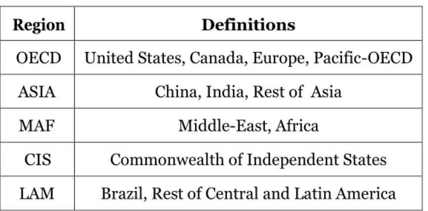
Imaclim-R is disaggregated into 12 regions (United-States, Canada, Europe, Pacific-OECD, Commonwealth of Independent States, China, India, Brazil, Middle-East, Africa, Rest of Asia, Rest of Central and Latin America). The results in this report were aggregated at the global level, or into 5 regions: OECD, CIS, MAF, ASIA and LAM. The definitions of the regions are summarized in Table 1.

9

Region Definitions

OECD United States, Canada, Europe, Pacific-OECD ASIA China, India, Rest of Asia

MAF Middle-East, Africa

CIS Commonwealth of Independent States LAM Brazil, Rest of Central and Latin America

Table 1: Description of regions used for the analysis

We used a method previously developed in (Rozenberg et al., 2014) to explore the multi-dimensional space affected by uncertain model input. In a first step, we identified the parameters that could in principle have an impact on results in terms of passenger and freight transportation pathways. The identified parameters were then gathered into parameter sets, seven in total, as presented in Table 2. For each parameter set, two or three alternatives were constructed, with contrasting parameter values. Two groups were chosen in order to relate to the Shared Socioeconomic Pathways (SSP) framework (O’Neill et al., 2017). They match the model parameters used to reproduce the different SSP, as in Marangoni et al. (2017). The transportation-specific parameters were collected into four groups using the ASIF decomposition (Schipper et al., 1999 ), depending on their a priori impact on (1) the Activity or volume of transport activity, (2) the Structure of transportation, i.e. changes in modal share, (3) the Intensity, i.e. the energy efficiency of transport modes, (4) the Fuels, i.e. the use of alternative fuels in the transportation sector. It should be noted transport-specific parameters do not directly prescribe the ASIF factors of transport sector emissions, the latter being also influenced by other determinants such as economic growth or energy prices.

10 Supplementary Material.

Sets of parameters Alternatives Parameters set

names Demography and productivity SSP1, SSP2 and

SSP3 Growth drivers

Determinants of mitigation challenges (fossil fuel reserves and markets, energy demand, low carbon technologies, except in the transportation sector) SSP1 (low challenges) or SSP3 (high challenges) Mitigation challenges Tr an sp or ta tio n s ect or p ar am ete rs Determinants of activity (volume of passenger and freight transportation) Low or high transportation demand Transport activity drivers Determinants of

structure (mode shares) Individual mobility dominated trend or shared-mobility oriented trend Transport structure drivers Determinants of intensity (energy efficiency)

Low or high energy

efficiency Transport intensity drivers Determinants of fuels

(alternative fuels) Low or high availability of alternative fuels Transport fuel drivers

Table 2: Description of parameter alternatives

The combinations of these parameter alternatives produced 96 baseline scenarios, i.e. scenarios in which no climate policy was implemented. In addition, in each of these 96 “future worlds”, we implemented two types of mitigation policies, making a total of 288 scenarios in all. Both types of mitigation policies were represented through a constraint on the global CO2 emission

11

policy cases, ‘High mitigation ambitions’1 _{and ‘Low mitigation ambitions’}2 _{differ in the}

stringency of the emissions constraint. In the rest of this text, the two mitigation scenarios will be referred to respectively as HMA and LMA.We considered results over the 2015-2080 timeframe because some mitigation scenarios appeared to be “not feasible” 3 _{beyond 2080.To}

be able to consider the whole set of scenarios, therefore, we restricted our analysis to the period 2015-2080.

To disentangle the underlying dynamics that lead to direct CO2 reduction, we applied index decomposition analysis for two years (2030 and 2050) between each mitigation scenario and the corresponding baseline and averaged the results over all scenarios. The factors analysed are the activity (pkm/capita), the mode shares, the energy intensity (EJ/pkm) and the fuel mix (g/EJ). We used the additive LMDI-I methods which is recommended because of multiple desirable properties in the context of decomposition analysis (see Ang (2004) for a review of the different existing methods and their properties). The alternative assumptions explored to construct the set of scenarios were designed to cover a relevant portion of the uncertainty space: the SSP framework is used to cover socio-economic uncertainties relating to demography, growth, and challenges to mitigation, the ASIF framework to focus on transportation-specific dynamics. However, even though this approach creates a wide range of scenarios, only part of the total uncertainty space is explored and the future might in reality bring changes that diverge

1 _{The case of “High mitigation ambitions” corresponds to an emission pathway between RCP 2.6 (Vuuren et al.,} 2011) and RCP 4.5 (Thomson et al., 2011). Cumulative CO2 emissions from 1870 to 2100 add up to 3800GtCO2.

This is between (i) the 3300GTCO2 value associated with a 33% probability of not exceeding 2◦C and (ii) the

4200 GtCO2 value associated with a 66% probability of not exceeding 3◦C (Pachauri et al., 2014). We do not

consider the more stringent constraint of an emission pathway following RCP2.6, because with such constraint a large number of scenarios were “not feasible” (see footnote 3 below).

2 _{The case of “Low mitigation ambitions” corresponds to the RCP4.5 (Thomson et al., 2011) emission pathway.} Cumulative CO2 emissions from 1870 to 2100 add up to 4600 GtCCO2. Global temperature is projected to

increase by a range of 1.7-3.2◦C from 1870 to 2100 with a median value of 2.4◦C (Pachauri et al., 2014).

3_{We consider here that scenarios are “not feasible” in modelling terms when the endogenous carbon price} increase from one year to another required to match the emissions trajectory is higher than 20%. The scenarios that are “not feasible” are essentially scenarios with parameters corresponding to the high mitigation challenges alternative.

12

from all 96 scenarios in this study. In particular, major global geopolitical developments might influence international transportation in ways that do not match any of the SSPs. Similarly, the spread of disruptive technologies such as autonomous vehicles, could potentially shape transportation behaviors outside the boundaries considered in this study (Fagnant & Kockelman, 2015). As with any modelling study, the results depend on the model structure used and on which sets of parameters are chosen to vary and on the alternative values tested. Obviously, the impact of an uncertain driver on the results depends on the numerical assumptions chosen for each state of the driver. Furthermore, scenarios cannot be associated with some objective probabilities. We are in a case of uncertainty, not a case of risk where the objective probabilities of parameters are known (Grübler & Nakicenovic, 2001; Cooke, 2015). Therefore, the distribution of results cannot be interpreted as an objective distribution of outcome probabilities and would have to be interpreted as subjective, in the Bayesian sense. In the results section, the mean of the distribution of results is plotted to make the figures more readable, but this mean is to be interpreted as implying a (subjective) equiprobability of all scenarios.

The results of the socioeconomic scenarios in terms of transportation activity serve as input for the second step of the methodology, which quantifies the investment needs that are consistent with these transportation activity pathways. The next subsection describes the method and data used in this second step.

2.2 Quantifying the investment needs for transportation

infrastructure underpinning the transportation activity

scenarios

The second step of the methodology consists in an ex-post analysis of the transportation activity scenarios produced. It is used to evaluate the investment needs, i.e. investment that

13

would be consistent with the given transportation activity scenarios, with certain target infrastructure utilization rates and adequate infrastructure maintenance. This is not the same approach as predicting future investment, which may be too small or too large relative to the levels required, resulting either in congestion and a deterioration in infrastructure quality in the first case, or in infrastructure underutilization and sunk costs in the second case.

The following transportation modes were considered: private vehicles, buses, bus rapid transit (BRT), rail, high-speed rail (HSR), and air transport for passengers; trucks and train for freight. Sea and air freight were not considered because of lack of data. The method used to compute investment needs proceeds in four steps: (1) compute mode share scenarios if they are not explicit, or not at the required disaggregation level, in input scenarios; (2) calibrate existing transportation infrastructure; (3) calculate the new construction required to fit the mobility scenarios; (4) calculate associated costs for construction, upgrade, operation, and maintenance of transportation infrastructure. Steps 2 to 4 are partly based on an approach to modelling infrastructure expansion in relation to scenarios for increases in transportation activity presented by Dulac (2013), with modifications and extensions as presented in the following subsections. The quantification was aggregated at the level of 5 world regions (OECD, CIS, Africa and Middle-East, Asia and Latin America). The transportation activities supplied by the Imaclim-R results were thus aggregated for these 5 regions for use as input into the analysis. We also incorporated the uncertain factors that determine investment needs by introducing alternative assumptions into the main parameters that play an a priori role in the four steps described above.

2.2.1 Modal share scenarios for passengers and freight

14

disaggregated into three modes for passengers (car, air, and other land modes) and into three modes for freight (air, sea, and land transportation). We made further assumptions to produce a more granular disaggregation of modes corresponding to the different infrastructures considered. To do this, we calibrated the respective shares to their 2015 values (see Supplementary Material, Table 7) and we considered two alternative scenarios for changes over time. In the first case, we consider the splits to remain constant over time. In the second case, we assumed that they evolve (linearly) towards levels in 2050 that are based on existing scenarios that represent a modal shift towards rail and BRT:

• Bus rapid transit share reaches 5% of bus share (Dulac, 2013);

• Rail freight share is 50% greater than road freight (UIC, 2016b), i.e. rail accounts for 60% of land freight transportation and trucks for 40%;

• Rail passenger share reaches 40% of public transport (IEA, 2012).

In the reports cited, these target mode shares were given at global scale. We applied them in the different regions of our model, assuming convergence between all regions. Modal shares were assumed to remain constant after 2050.

2.2.2 Calibration of existing transportation infrastructure capacity

The different types of infrastructures considered and the associated units of measurement are summarized in Table 3. The values for transportation infrastructure capacities calibrated in 2015 for the 5 regions of our model are also presented.

Mode Unit of stocks ASIA CIS MA

F LAM OECD Road thousand lane.km 16,172 3108 2290 1489 24,000 BRT thousand trunk.km 1.24 0 0.30

9 1.8 2.05 Rail thousand track.km 187 159 57.1 84.5 663.7 High speed rail thousand track.km 36.43 0 0 0 24.77

15

Table 3: Calibration of infrastructure stock for the year 2015 from different databases4

Following Dulac (2013), five, three and two lanes were assigned respectively to highways, primary road networks, and other roads, when complete data on different types of road were available. Otherwise, five and two lanes were assigned respectively to highways and the rest of the road network. Technically, BRT infrastructure was considered to be roadway. However, BRT systems require their own investment and involve high-capacity buses running in separate lanes isolated from other road traffic. For rail infrastructure, both urban and non-urban rail were considered and aggregated, with the exception of high-speed rail infrastructure, which was considered separately. Airports were included in this study but were not considered as a stock but as a fixed cost per unit of air passenger travel, following Broin & Guivarch (2017).

2.2.3 New build needs underlying the mobility scenarios

First, we aggregated private vehicles, buses, and trucks to evaluate the rate of utilization of the road infrastructure. To do so, we converted the data in passenger.kilometer (pkm) and tons.kilometer (tkm) to vehicle.kilometers (vkm) using vehicle occupancy factors.5

Then, we defined a “desirable” infrastructure utilization rate and the speed at which it could be achieved from the current utilization rate. The current road utilization rate as reflected in data for distances travelled and infrastructure capacities varies greatly between world regions, from 150,000 vkm/paved lane.km for India to more than 1,000,000 vkm/paved lane.km for Latin America (Dulac, 2013). A first possible explanation for this heterogeneity is traffic structure.

4 _{UIC (2016a), UIC (2017) CIA (2017) and EMBARQ (2017) for ASIA, CIS and MAF; EMBARQ (2017) and BID} (2016) for LAM; UIC (2016a), UIC (2017) and IRF (2009) for OECD

5 _{The average payload for a truck is assumed to be 13 tons (IEA, 2009). The average passenger occupancy for} a bus used is 20 (Schipper et al., 2011). For car occupancy, we use trends in regional values from the Imaclim-R scenario inputs. The unit value of passenger car road occupancy, which is a unit that gives the vehicle equivalent in terms of cars, is assumed to be 2.5 for a truck and 2 for a bus, based on values from (Adnan, 2014)

16

In freight activity, for example, 79% of goods are transported by truck in Latin America (ITF, 2017), whereas 36% are transported by rail in India (Mc Kinsey, 2010). This mode structure has an influence on road occupancy. A second possible explanation is that the road quality defined as paved differs between countries (Schwab & Sala i Martin, 2016).

There is uncertainty about what utilization rate can be considered as “desirable”. Indeed, high road utilization rates are a source of congestion, which is associated with financial costs and welfare losses caused by (i) vehicle delays, (ii) greater capital depreciation, (iii) congestion-related accidents, and (iv) the negative impact of congestion on the location of economic activities in a town (Bilbao-Ubillos, 2008). We chose to consider the two different levels of 600,000 and 900,000 vkm/paved lane.km as desirable utilization rates. A target road utilization rate of 300,000 vkm/paved lane.km has also been tested. However, we assumed that the lowest utilization rates on international comparisons, such as those of India and China, would increase as a result of surges in mobility demand from private motorization. We therefore did not consider this value in our results. We also did not consider higher desirable utilization rates, such as current levels in Latin America. The region has experienced lack of investment in recent decades (Perrotti & Sánchez, 2011), so we do not see the current road utilization rate as a reasonable long-term target, but rather as an indicator of congestion or poor infrastructure quality.

The BRT trunk.km occupancy target was assumed to be 120,000 bus vkm per BRT km (Dulac, 2013) with roughly 100 people per bus. The BRT system also uses the road, but requires a separate lane, so there is no influence on road occupancy.

For rail transportation, passenger-kilometers and ton-kilometers were summed together in transport units following UIC (2016b), assuming that 1 ton-kilometer is equivalent to 1 passenger-kilometer in terms of occupancy. Current rail occupancy levels range from less than 350,000 pkm and tkm per track-km for Eastern Europe to more than 30 million pkm and tkm in

17

Mexico (Dulac, 2013). This big disparity in rail occupancy could arise from different factors: infrastructure stocks, operating strategies, etc. High and low values for rail utilization rates (30 and 5 million pkm-tkm/track-km) were tested in our model.

It is important to note that we use average infrastructure occupancy rates and that these values may mask some heterogeneity of use in the road network, particularly between urban and rural areas. For instance, an increase in the road occupancy rate induced by a growth in road traffic concentrating on part of the already saturated network could lead to new constructions and therefore additional costs not taken into account in our study. Similarly, an increase in traffic on lightly used road infrastructure would not lead to additional construction costs. We thus assumed, using the average rate, that these two effects offset each other at the regional level. The speed at which the “desirable” utilization rates may be reached from current utilization rates was assumed to be either 35 (target values reached in 2050) or 65 years (target values reached in 2080). The changes towards the target utilization rates were assumed to be linear. At each time step, the combination of the desirable utilization rate, the speed assumptions, and the utilization rate from the previous time step, determine the objective infrastructure occupancy targeted.

Finally, the ideal infrastructure stock is calculated in the model, at each time step, as the ratio between transportation activity and the infrastructure occupancy objective. The actual infrastructure stock from the previous time step is compared with the ideal infrastructure stock. In the case of under-utilization (infrastructure stock greater than ideal infrastructure stock), new construction is not necessary and the occupancy rate can increase. In the case of over-utilization (infrastructure stock smaller than ideal infrastructure stock), new construction is needed. The calculated need for new construction is then compared with the maximum density of infrastructure in the region and reduced if the maximum would be exceeded. The rail and road density limits applied are based on values from Dulac (2013) (see Supplementary

18 Material, Table 8).

For airports, the need for new construction is not calculated ‘physically’ because of lack of data on airport stock and the constraints on infrastructure capacity. It was assumed that passenger activity was the unique driving force for airport construction.

2.2.4 Costs associated with new construction, upgrade, reconstruction, and maintenance

The assumptions for the unit costs of infrastructure are taken mainly from Dulac (2013) and represent the yearly investments per unit of infrastructure capacity. Infrastructure costs in the different regions are summarized in Table 4.

For road investments, the costs are split into three categories: new build, up- grade/reconstruction, and operation and maintenance. Upgrade and reconstruction are less expensive than new construction because they involve work on existing infrastructure. It was assumed that road infrastructure requires reconstruction or upgrade every 20 years. For rail investment, only new construction costs and operation/maintenance were considered, following Dulac (2013) who suggested that rail is generally maintained through regular investment in operation and maintenance and is replaced in sections when track is no longer operable.

For BRT investments, reconstruction costs were assumed to account for half of BRT capital development costs. Infrastructure lifespan was also assumed to be 20 years.

Airport costs are divided into two categories, one for new construction and one for stock maintenance. The price for new construction used is per additional passenger.kilometer and the price for maintaining the stock is per total passenger.kilometers. Because of lack of data, we used values from OECD countries for all regions.

19

Cost category Mode Unit ASIA CIS MAF LAM OECD

New Build

road thousand usd/lane.km 1100 1000 1100 1200 1200 brt thousand usd/trunk.km 7000 7000 7000 7000 15000 hsr thousand usd/track.km 24000 24000 24000 24000 24000 rail thousand usd/track.km 4500 4000 4500 5000 5000

air usd/pkm 0.25 0.25 0.25 0.25 0.25 Upgrade and

Reconstruction

road share of new build cost 0.008 0.0075 0.009 0.008 0.009 brt share of new build cost 0.025 0.025 0.025 0.025 0.025

Operation and Maintenance

road share of new build cost 0.0075 0.0075 0.0075 0.0075 0.0075 brt share of new build cost 0.01 0.01 0.01 0.01 0.01 hsr share of new build cost 0.004 0.004 0.004 0.004 0.004 airports share of new build cost 0.01 0.01 0.01 0.01 0.01

Table 4: Costs of infrastructures – Sources: Broin & Guivarch (2017), Dulac (2013)

Three different assumptions for cost changes over time were considered in this study: constancy over time, increase of 50% in 2100 relative to 2015 levels, and decrease of 50% in 2100. Cost increases and decreases were assumed to be linear until 2100. An increase in infrastructure costs over time represents the case where, with infrastructure network development or over time, construction costs (including materials and labor) increase, or the marginal infrastructure becomes more complex and thus more costly. A decrease in infrastructure costs over time represents the case where progress through learning-by-doing is a dominant effect.

20

Uncertain factors Option 1 Option 2 Option 3 Parameter names

Transport mode shares Constant Modal shift Modal shift

Target road utilization rate (vkm/paved lane.km)

600,000 900,000 Road target

Target rail utilization rate (106 _{pkm+tkm/track.km)}

5 30 Rail target

Delays to reach target

utilization rates (years) 35 65 Delay

Change in unit cost for roads Increase by 50% Constant Decrease by 50% Road costs

Change in unit cost for rail Increase by 50% Constant Decrease by 50% Rail costs

Table 5: Summary of uncertain factors considered for investment analysis

To explore the uncertainty space, we combined all alternative options considered for the six un- certain factors, as summarized in Table 5. We therefore evaluated 144 quantifications of investment needs for each transportation activity scenario. Performing quantification for all 288 transportation activity scenarios arising from the previous step, we built a database of 144*288 (41,472) quantifications of investment need. The limitations of this method of building a set of scenarios are the same as those already described in the previous section. Furthermore, it should be noted that we consider all combinations of the investment analysis parameters together with all the socio-economic worlds included: the parameter sets are varied independently of each other. Doing so neglects possible cross-correlations between some of the sets and tends to produce a range of results that is too broad, because some combinations may not be internally consistent. However, removing combinations that appear less internally consistent may miss plausible surprising futures. We therefore considered the full set of scenarios produced in the analysis.

21

2.3 Global sensitivity analysis to identify the main

determinants of investment needs

In order to identify the main determinants of investment needs, we conducted a global sensitivity analysis. Our chosen output metrics for this analysis are total infrastructure costs and annual investment needs relative to GDP (averaged over time). The inputs are the parameters or group of parameters described in Tables 2 and 5. We chose not to use the so-called “One At a Time” sensitivity analysis design, where each input is varied while the others are fixed. Although widely used by modelers, its shortcomings have been extensively described in the statistical literature (Saltelli & Annoni, 2010). An alternative is the Standard Regression Coefficients Approach (SRC), used for instance by Pye et al. (2015) to conduct a sensitivity analysis for an energy system model. According to these authors, the advantages of this metric are the lack of complexity in their calculation and their independence of the units or scale of the inputs and outputs being analyzed. However, the SRC approach is ill-suited to our model, because it is based on a linear relationship between the output and the inputs (Iooss & Lemaître, 2015), while the R2 coefficient of determination allows us to invalidate the linear hypothesis with values obtained that are lower than 0.8 in our case.

We therefore chose an approach that is more complex, but does not require a linear hypothesis: the variance-based decomposition method proposed by Sobol (2001) and described in Saltelli et al. (2008). The main advantage of this method is that it is robust to both linear and non-monotonic relationships between model inputs and outputs (Iooss & Lemaître, 2015). The proportion of total variances is attributed to individual input as well as to interactions between those factors. First-order effect indices represent the output variance attributable to each input without considering interactions with other inputs. Total effect indices represent the total contribution to output variance by each input, including interactions with all other inputs. Calculations were done using the SALib package in Python (available at

22

github.com/SALib/SALib). We chose to display the results with radial convergence diagrams, which are drawn using R DataVisSpecialPlots (available at

https://github.com/calvinwhealton/DataVisSpecialPlots).

3 Results

3.1 Socio-economic scenarios and transportation pathways

The 96 baseline scenario results range from about 3100 GtCO2 to about 6300 GtCO2 in terms

of cumulative CO 2 emissions from fossil fuel combustion between 2001 and 2080 (Figure 1a).

Emission levels in 2050 range from 1.3 to 3 times 2010 levels. This range is comparable to the range covered by the baseline scenarios in the IPCC AR5 database, in which 2050 emissions range between 1.1 and 3.1 times 2010 levels. In the baseline scenarios, global GDP in 2080 ranges from 2 to 7.5 times its 2001 value (Figure 1b). This range of results is also comparable with the range covered by baseline scenarios in the IPCC AR5 database, where global per capita GDP in 2080 ranges from approximately 2.5 to 8 times its 2001 value.

The fossil CO 2 emissions from the baseline transportation scenarios range from 11.6-19.4 Gt

CO2 per year in 2050 (Figure 1c), which is comparable with the range of 11-18 Gt CO2 found by

Yeh et al. (2017). In contrast with global CO2 emissions trajectories that are arrived at for all

mitigation scenarios with the same ambition, emissions trajectories for the transportation sector differ between scenarios in the two groups of mitigation scenarios. Indeed, CO2 emission

mitigation efforts are not always the same from one economic sector to another, and depend on the combination of assumptions made on the values of groups of parameters. For instance, in cases where the parameters are such that low-carbon technologies in the power sector have limited potentials and higher costs, less mitigation is done in the power generation sector,

23

which requires more mitigation in other sectors in order to maintain the global constraint on total emissions.

Transportation activity for baseline scenarios reaches values in 2080 in a range from 2 to 4 times the 2001 value for passenger mobility and from 5 to 10 times the 2001 value for freight activity (Figures 1d and 1e). Global passenger mobility is expected to increase by 1.75-2.33 times from 2010 to 2050, rising from approximately 48 trillion pkm in 2010 to 84-115 trillion pkm in 2050, which is slightly smaller than the range of 1.9-3.3 covered by the baseline scenarios from Yeh et al. (2017). Transportation activity is reduced in 2080 in low and high mitigation ambition scenarios compared with baseline scenarios with a median decrease value of respectively 26.4% and 33.2% for passengers and 41.2% and 46.9% for freight. In figures 2a and 2b, activity reduction and low-carbon alternative fuels appear to be the main factors for CO2 reduction for both freight and passenger transportation. Their contributions are respectively greater than 25% in average for both passenger and freight in 2030 and 2050. The greater CO2 reduction in the HMA scenarios compared to the LMA scenarios is achieved mainly through a greater reduction in activity in the short term (2050) for freight and passenger and a higher contribution of energy efficiency in the long term (2080) for passenger transport. It should be noted that the contribution of modal shift may be underestimated given the high level of aggregation for public transportation and freight transport (that aggregate all terrestrial modes including road and rail) in Imaclim imposed by the data of energy accounting.

24

(a) CO2 emissions from fossil fuel combustion _{(b) GDP}

(c) CO2 emissions from the transport sector (d) Passenger transportation activity

(e) Freight transportation activity

Figure 1: Evolution over time of global socio-economic outputs from Imaclim scenarios; median (solid line) and max/min (dashed lines).

25

(a) Passenger (b) Freight

Figure 2 LMDI decomposition analysis of ASIF factors underlying CO2 emissions reduction in the

mitigation scenarios compared to baseline scenarios. The factors analysed are the activity (pkm/capita), the modes shares, the energy intensity (EJ/pkm) and the fuel mix (g/EJ).

3.2

Effects of low-carbon policy on investments

In the case of the baseline scenarios, we found global investment needs of between $1 trillion and $4 trillion per year on average, with a median value of $1.9 trillion per year. Those results are comparable with the $2.11 trillion value in Dulac (2013) (whose study also includes car parks, but not airports), and in Dobbs et al. (2013) of $1.35 trillion per year (including road, rail, and airports). Under low carbon policy, we obtained values (i) between $0.92 and $3.4 trillion per year with a median value of $1.7 trillion for LMA scenarios and (ii) between $0.87 and $3.4 trillion per year with a median value of $1.6 trillion for HMA scenarios. This range of results is comparable with the values of $1.8 trillion from Dulac (2013) and of $2.5 trillion from IEA (2016) obtained for rail and road infrastructures under a low-carbon scenario.

To have an order of magnitude for comparison, global Gross Fixed Capital Formation amounted to 18.7 trillion USD2016 in 2016, representing approximately 23% of world GDP. The main shares of investment are in road and rail infrastructures, with values between 42% and 95% and between 2% and 49% respectively. When considered relative to GDP, the annual

26

investment needs averaged over time are similar for baseline, LMA, and HMA scenarios with values between 0.7% and 2.5% of GDP.

For each combination of uncertain parameters, we computed the relative variation in investment needs between each mitigation scenario and the corresponding baseline (i.e. the baseline with the same combination of uncertain parameters), for each region and at the global scale (Figure 3a). We find that climate policies lead to a reduction in cumulative spending needs on transportation infrastructures and confirm the results from past studies (Dulac, 2013, Broin & Guivarch, 2017). In addition, we add that this effect is robust to the different assumptions on the uncertain parameters considered. The relative decrease in investment needs ranges from 2% to 25% for LMA scenarios, and from 5% to 33% for HMA scenarios. The reduction in investment needs comes mainly from reduced need for investment in roads, followed by rail and airports: the contributions of each represent respectively between 40% and 99%, between 0.3% and 45%, and between 0.5% and 15% of the total decrease. In the case of HMA scenarios, it translates into an annual decrease in investment needs of between $74 and 976 billion/year for road, between $4 and $206 billion/year for rail, and between $8 and 66 billion/year for airports (Figure 3b). Investments in high speed rail infrastructures increase in 67% of the scenarios with a maximum difference of $39 billion/year which is below the values of roads investments decreases.

This result – a decrease in investment needs under mitigation scenarios – is also valid at the regional scale for most of the scenarios but with different magnitudes (Figure 3a). Investments in MAF under ambitious mitigation policies are reduced by [35%-65%] whereas in OECD the variation is less than 10%. In a few cases for ASIA, investment needs are higher under climate policies with a maximum increase of 3%. Most (83%) of these cases are associated with the assumptions of an increase in rail costs over time, a high target road utilization rate, and low energy efficiency in the transportation sector.

27

(a) (b)

Figure 3: Comparison of cumulative investment needs between mitigation scenarios and their corresponding baselines (a) Relative difference in cumulative investment needs (a negative value indicates that the investment is lower in the mitigation scenario); (b) Contribution of each infrastructure type to total annual investment difference

The overall decrease in investment needs is brought about in particular by a reduction in transportation activity in a low carbon-world, according to Figures 1d and 1e. The largest decreases in investment needs come from road infrastructures. This decrease is amplified for ASIA, CIS, and MAF by a mode shift from personal vehicles to low-carbon modes (public transit and non-motorized modes) triggered by climate policies (see Table 9 in Supplementary Material). However, the associated mode shift induced by climate policies can partly offsets the effect of activity reduction and tends to increase overall investment (see figure 5 in the

Supplementary Material). .

We did not correlate here the climate policy scenario and the evolution of mode shares including a modal shift from road to rail for public transportation and freight (see section 2.2.1 for details). Indeed, modal shift can be sought for other reasons such as congestion. We

28

analyzed as well investments difference for HMA scenarios assuming a correlation between this modal shift and climate policy. We obtained that the results of investments decrease remains valid for most of the scenarios at the global scale and for all regions except OECD (see figure 2 in the supplementary material). Indeed, by triggering modal shift to rail, the implementation of climate policy tends to reduce investment needs at the global scale but to increase them in the OECD region which is a similar result to the one obtained in IEA (2016) for the Nordic region.

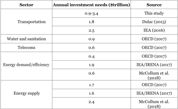
Sector Annual investment needs ($trillion) Source

Transportation

0.9-3.4 This study

1.8 Dulac (2013)

2.5 IEA (2016)

Water and sanitation 0.9 OECD (2017)

Telecoms 0.6 OECD (2017) Energy demand/efficiency 0.4 OECD (2017) 1.9 IEA/IRENA (2017) 0.6 McCollum et al. (2018) Energy supply 1.7 OECD (2017) 1.6 IEA/IRENA (2017) 2.4 McCollum et al. (2018)

Table 6: Comparison of transportation infrastructure investment needs with those of other sectors under a low- carbon scenario

It should be recalled that we did not take into account the additional investments associated with energy efficiency and the use of alternative fuels because they are already included in the existing studies about investments for energy infrastructures in low-carbon scenario. If

29

included, those costs may nuanced the overall results of lower investments in mitigation scenarios in the transportation sector.

30

Though the investment needs are lower in mitigation scenarios compared with baselines, they are significant by comparison with other sectors, notably telecommunications and water infrastructures, where the needs quantified in the literature are lower than our lowest value (Table 6). The needs in the transportation sector even appear to be of the same order of magnitude as the investment needed in the energy sector. A notable difference with the energy sector is that investment needs decrease for transportation infrastructure in low-carbon pathways compared with baselines, whereas they increase in the energy sector. Nonetheless, financing these low-carbon investment needs may remain a challenge (Granoff et al., 2016). In the next section, therefore, we analyze regional investment needs in low-carbon pathways in order to identify cases of high and low investment needs and their main determinants.

These differences between regions in the level of investment needs can be partly explained by regional characteristics of the transportation sector, summarized in Table 7. Transportation intensity of GDP varies between regions and reflects their economic structure, with freight intensity depending mainly on both per capita income and the service sector’s share of GDP (ITF, 2015). CIS has the specificity of combining a high initial rail utilization level and freight activity that mainly relies on rail infrastructures, with a mode share close to 90% (supplementary material, Table 7). Moreover, its freight intensity of GDP is more than twice the values of other regions. This combination leads to high investment needs, and a larger share allocated to rail infrastructures than in other regions (Figure 4b). Investment needs are high in MAF as well, but the factors explaining its transportation structure are different. The region has a high passenger intensity of GDP. Moreover, MAF combines high initial road occupancy and a road-oriented transportation system with road shares of 88% for land freight and 94% for passenger land transportation (see supplementary material Table 7). This combination leads to higher and more road-oriented investment needs (Figure 4b). High investment needs could have been expected in Latin America – the region with the highest initial

31

road utilization rate – but low land freight intensity offsets this effect. Results for OECD can be explained by relatively low values for both freight and passenger intensity of GDP.

(a) (b)

Figure 4: Comparison of investment needs between regions for HMA scenarios; (a) Distribution of annual investment needs relative to GDP (average on 2015-2080); (b) Allocation of investment between transportation modes.

ASIA CIS MAF LAM OECD

Road utilization rate in 2015 (thou- sand vkm/lane km)

200 300 900 1500 550

Rail utilization rate in 2015 (thou- sand pkm+tkm/track km)

20,000 25,000 10,000 6,000 6,000

Land freight intensity (mean) in 2030/2070 (tkm per US$2005)

0.71/0.65 1.68/1.72 0.71/0.64 0.47/0.3

8 0.18/0.16 Passenger intensity (mean) in

2030/2070 (pkm per US$2005)

1.36/1.09 0.88/0.7 1.47/0.95 1.08/0.68 0.45/0.27

Table 7: Transportation structure characteristics obtained in the model for the five regions considered in this study.

32

In order to analyze the uncertain factors determining the total variance (or total uncertainty) of results for each region, we conducted a global sensitivity analysis, following the Sobol method described in section 2.3. First, second-order and total-order indices for investment needs relative to GDP are summarized in Figure 5. Results for total cumulative investments as output are given in the supplementary material. We find that the target rail utilization rate and road costs are influential determinants for all regions. For ASIA, the three parameters that most influence the results are the changes in road costs, the mitigation challenges, and the growth drivers, with total index values of 29% [90% confidence interval of 2.5%], 30% [2%], and 17% [1%] respectively. The absence of black lines shows that the interactions between parameters are limited, the second-order indices being less than 5%. The target rail utilization rate is the main determinant in CIS with a total-order index of 73% [6%]. This result confirms the importance of rail investment in the total infrastructure expenditure needs for the region. Figures 5c and 5d show that the determinants are similar for LAM and MAF. Changes in road costs and target infrastructure utilization rates (rail and road) do most to determine the results for these two regions with values of 17% [1%], 34% [3%], and 31% [2%] for MAF, and 18% [2%], 27% [2%], and 20% [2%] for LAM. For the modal shift parameter, we quantify first/total order indices as 4% [3%]/13% [1%] for LAM and 4% [3%]/18% [2%] for MAF. The interactions between this parameter and the target rail utilization rate make the modal shift assumption influence total uncertainty more than would be apparent in a one-at-a-time sensitivity analysis (figures 5c and 5d). For the OECD region, the main determinants of investment are the changes in road costs, the target infrastructure utilization rates, the growth drivers, and transportation structure (figure 5e).

The groups of parameters varied in the Imaclim-R model to construct transportation activity pathways have limited influence on the investment needs evaluated ex-post, mainly because general equilibrium effects and interactions with other sectors are at play (e.g. macroeconomic

33

rebound effect in the case of improved fuel efficiency). Notable exceptions are the growth drivers (especially for ASIA, LAM and OECD regions), the mitigation challenge (for ASIA), and the transportation structure (for LAM and OECD). The demography and productivity assumptions used are such that they lead to higher GDP growth associated with relatively lower transportation intensity when the growth drivers are as in SSP1, compared with SSP2, and in SSP2 compared with SSP3. Investment needs for transportation infrastructure relative to GDP are therefore lower in scenarios with SSP1-like growth drivers and higher in scenarios with SSP3-like growth drivers. Higher mitigation challenges lead to a higher macroeconomic cost for reaching a given mitigation objective, hence lower GDP, so investment needs relative to GDP are therefore higher. This effect is particularly visible for ASIA, for which mitigation costs increase in the ‘high mitigation challenges’ cases. The assumption regarding transportation structure parameters leads to a slower increase in passenger.kilometers traveled in the case of a structure oriented towards shared mobility, therefore reducing the need for investment in for roads. This reduction has a sizeable effect on overall investment needs for Latin America (a region where road utilization rates at the beginning of the period were very high) and for OECD, but only when combined with low target road utilization rates for the region.

Road costs are an influential parameter in all regions. This result was to be expected because road investments account for the main proportion of investment needs (figure 4b). A change in the price of road infrastructure therefore leads to significant variation in total investment costs. Research and development policy focused on less expensive road construction technologies could be relevant for reducing the cost of investment.

The influence of the target rail utilization rate on all regions needs to be qualified to the extent that it is a result of the two alternative values chosen here for this parameter. The result is indeed influenced by the difference between the two values, the high target being 6 times greater than the low target. Moreover, the target of 5 million pkm+tkm/track.km is below the

34

initial rail utilization rates (Table 7) of all the regions and increases the importance of this parameter, because it implies the need for investment even in the absence of a rise in transportation activity. In a previous version of this study, we also analyzed scenarios with a lower target of 300 thousand vkm/lane.km for road occupancy. This value was low compared with 2015 road occupancy levels (Table 7), with the result that this parameter had a greater influence on the outcomes. The importance of target rail utilization rates for overall investment needs can be interpreted in two ways. A first possible interpretation is that aiming to decrease the rail infrastructure utilization rate may seem unrealistic in terms of investment needs. This is particularly the case for the CIS and MAF regions where investment needs are then higher than actual investments (as a share of GDP) observed in the past. A second interpretation is more policy-related and identifies an increase in rail utilization rates as a possible lever for reducing investment needs. For regions other than CIS and MAF, optimizing the rail network in order to achieve higher utilization could thus be an option to avoid high-cost pathways. Similarly, for the target road utilization rate parameter, our results highlight the fact that, since LAM and MAF had the highest levels in 2015, reducing utilization rates inevitably leads to a sharp increase in investment needs.

The big influence of modal shift from road to rail for public transit and freight, associated with a strong interaction between this parameter and the rail occupancy target in the LAM and MAF regions, can be explained by the results summarized in Table 8. For both regions, this mode shift has an opposite effect depending on the rail utilization rate target: it decreases annual investment needs in the cases of high target rail occupancy and increases investment needs otherwise. The magnitude of the effect also differs depending on the rail utilization target: the decrease is relatively small whereas the increase is larger (Table 8). Mode shift may be sought for other reasons than CO2 reduction (for instance, congestion relief, air quality improvement

35

needs only if combined with actions to increase rail infrastructure utilization rates. Otherwise, there is a risk that modal shift could lead to higher investment needs.

Scenarios considered MAF LAM

Low rail occupancy target + no modal shift 2.6% 1.8% Low rail occupancy target + modal shift 3.4% 2.4% High rail occupancy target + no modal shift 2.3% 1.6% High rail occupancy target + modal shift 2.2% 1.5%

36

(a) ASIA (b) CIS

(c) MAF (d) LAM

Figure 5: Sobol method global sensitivity analysis results for each region, for investment needs relative to GDP. Filled nodes represent the first-order indices and rings the total-order indices. Lines represent second-order indices arising from interactions between inputs. Width of lines indicates the second-order indices. Only the second-order indices greater than 5% of total variance are represented. For a description of the parameters, see the last columns of tables 2 and 5.

37

4 Conclusion

In this study, we quantified the needs for investment in transportation infrastructures between 2015 and 2080 along high and low carbon pathways, considering road, rail track, BRT lanes, high-speed rail, and airports, at the global level and for five world regions. We first constructed transportation activity trends using a set of socio-economic scenarios built using the Imaclim-R model, an integrated assessment model that explicitly represents the transportation sector, including its non-price determinants, and captures its principal interactions with the rest of the economy. We then performed an ex-post valuation of the annual investment needs consistent with these trends in transportation activity. We took uncertainty into account by combining alternative assumptions regarding influential parameters in both steps of our methodology. We confirm the finding of the few analyses carried out on the subject of investments in low-carbon transportation infrastructure, that global cumulative investment needs are reduced in low-carbon scenarios compared with high-carbon pathways. We additionally show that this result is robust to the different assumptions regarding uncertain parameters that influence transportation patterns and infrastructure expenditure. This result is also valid at the regional level, for the five regions we analyzed. The overall diminution in investment needs is brought about in particular by a reduction in transportation activity in a low-carbon world. The biggest decreases in investment needs are in road infrastructures.

In low-carbon pathways, investment needs relative to GDP differ between regions, with lower needs for OECD, high needs for CIS and MAF, and intermediate values for ASIA and LAM. The uncertainty ranges and the factors of uncertainty also differ between regions. The uncertainty ranges are larger for CIS and MAF, and lower for OECD. For those regions, the results for investment needs are particularly high by comparison with the historical values for investment in transportation infrastructures in most of the countries.

38

We took the analysis further by using a global sensitivity analysis to identify the main determinants of investment needs in the different regions studied. Target rail utilization rate and road construction costs determine investment needs in all the regions, but differ in the magnitude of their contributions to uncertainty. Other determinants of investment needs are region-specific, such as mitigation challenges for ASIA, transportation structure for OECD, and modal shift from road to rail for LAM and MAF. For these regions, we found a strong interaction between modal shift and the long-term rail target, the modal shift tending to lead to an increase or decrease in investment depending on the target rate of rail use.

We did not consider in this study additional investments related to energy efficiency or infrastructures for the use of alternative fuels. To obtain a comprehensive assessment of the costs related to the transport sector in a low-carbon world, these elements should be integrated. Inevitably, our results are conditional on the structures of the models we used, and on the alternative values we considered for the groups of uncertain parameters. They can therefore not be taken literally as definitive quantifications, and could be investigated further with alternative model structures or assumptions. In addition, the calibration for initial infrastructure occupancy levels is based on data collected from different sources, which potentially differ in their completeness and quality. If transportation activity is underestimated and/or infrastructure stocks overestimated in the data, we may underestimate the initial infrastructure utilization rates. This may be the case for ASIA, which in our data has very low initial road use. Conversely, utilization rates may be overestimated if transportation activity is overestimated and/or infrastructure stocks underestimated. For instance, this may be the case for LAM in our data. The lack of data for some regions or inconsistency between sources call for a serious effort to obtain open and comprehensive data on transportation infrastructures. In our methodology, we do not account for the feedback effect of infrastructure development costs on economic activity, because the investments consistent with transportation activity