HAL Id: hal-01374450
https://hal.archives-ouvertes.fr/hal-01374450
Submitted on 3 Oct 2016
HAL is a multi-disciplinary open access
archive for the deposit and dissemination of sci-entific research documents, whether they are pub-lished or not. The documents may come from teaching and research institutions in France or
L’archive ouverte pluridisciplinaire HAL, est destinée au dépôt et à la diffusion de documents scientifiques de niveau recherche, publiés ou non, émanant des établissements d’enseignement et de recherche français ou étrangers, des laboratoires
Positive and unlabeled learning in categorical data
Dino Ienco, Ruggero G. Pensa
To cite this version:
Dino Ienco, Ruggero G. Pensa. Positive and unlabeled learning in categorical data. Neurocomputing, Elsevier, 2016, 196 (july), pp.113 - 124. �10.1016/j.neucom.2016.01.089�. �hal-01374450�
Positive and unlabeled learning in categorical data
Dino Iencoa,c, Ruggero G. Pensa∗b
aIRSTEA Montpellier, UMR TETIS - F-34093 Montpellier, France Tel. +33(0)4.67.55.86.12 – Fax. +33(0)4.67.54.87.00
dino. ienco@ irstea. fr
bDept. of Computer Science, University of Torino - I-10149 Torino, Italy Tel. +39.011.670.6798 – Fax. +39.011.75.16.03
pensa@ di. unito. it
cLIRMM Montpellier, ADVANSE - F-34090 Montpellier, France
Abstract
In common binary classification scenarios, the presence of both positive and negative ex-amples in training data is needed to build an efficient classifier. Unfortunately, in many domains, this requirement is not satisfied and only one class of examples is available. To cope with this setting, classification algorithms have been introduced that learn from Posi-tive and Unlabeled (PU) data. Originally, these approaches were exploited in the context of document classification. Only few works address the PU problem for categorical datasets. Nevertheless, the available algorithms are mainly based on Naive Bayes classifiers. In this work we present a new distance based PU learning approach for categorical data: Pulce. Our framework takes advantage of the intrinsic relationships between attribute values and exceeds the independence assumption made by Naive Bayes. Pulce, in fact, leverages on the statistical properties of the data to learn a distance metric employed during the classification task. We extensively validate our approach over real world datasets and demonstrate that our strategy obtains statistically significant improvements w.r.t. state-of-the-art competi-tors.
Keywords: positive unlabeled learning, partially supervised learning, distance learning, categorical data
1. Introduction
In common binary classification tasks, learning algorithms assume the presence of both positive and negative examples. Sometimes this is a strong requirement that does not fit real application scenarios. In fact, the process of labeling data is a money- and time-consuming activity that needs high-level domain expertise. In some cases this operation is quick, but usually, definining reliable labels for each data example is a hard task. In the worst case, extracting examples from one or more classes is simply impossible [1]. As a consequence, only a small portion of a so-constituted training set is labeled. As a practical example of this
phenomenon, let us consider a company that aims at creating an archive of researchers’ home pages, using web-crawling techniques. Once downloaded, a web page should be classified to decide whether it is a researcher’s home page or not. In such a context, the concept of positive example is well defined (the researcher’s home page) while the idea of negative example is not well-established [2] because no real characterization of what is not a home page is supplied. The same problem occurs when trying to classify biological/medical data. Usually a biologist (or a doctor) can comfortably supply positive evidences of what she wants to identify but she is not able to provide negative examples. A known example of this scenario is the classification of vascular lesions starting from medical images [3], where labeling vascular lesions accurately could take more than one year, while it is relatively easy to recognize healthy individuals. In these scenarios, defining a method to exploit both positive and unlabeled examples could save precious material and human resources and the expert may focus her effort to only define what is good, skipping the ungrateful task of recognizing what is not good.
To deal with this setting, the Positive Unlabeled (PU) learning task has been introduced [4]. Roughly speaking, PU learning is a binary classification task where no negative ex-amples are available. Most research works in this area are devoted to the classification of unstructured datasets such as documents represented by bag-of-words, but similar scenarios may occur with categorical data as well. Imagine, for instance, a dataset representing census records on a population. An analyst can comfortably provide reliable positive examples of a targeted class of people (e.g., unmarried young professional interested in adventure sports), but identifying plausible counterexamples is not as easy. However, very few PU learning approaches are designed to work on attribute-relation data (such as categorical datasets). Unfortunately the techniques proposed in text classification are not directly applicable to the context of attribute-relation datasets. These approaches, in fact, employ metrics, such as the cosine distance, that are not well suited for categorical data where, in addition, there is no standard definition of distance [5]. This limitation makes it impossible to apply works on document classification to categorical data directly. The few works that deal with PU learning in attribute-relation domains are principally based on Naive Bayes classifiers. The major limitation of this kind of approaches is that algorithms based on Naive Bayes assume that attributes are mutually independent. To the best of our knowledge, no effort was de-voted to the implementation of other models or the extension of previously defined models from document analysis.
In this paper we introduce a new distance-based algorithm, named Positive Unlabeled Learning for Categorical datasEt (Pulce). Our work aims at filling the gap between the recent and well-established advances in document classification and the preliminary status of works existing for attribute-relation data. In particular, we address the problem of classifying data described by categorical attributes, which also includes the case of discretized numerical attributes, leading to a general framework for attribute-relation data. The core part of our approach is an original distance-based classification method which employs a distance metric learnt directly from data thanks to a technique recently presented by Ienco et al. [6]. Originally, this technique was designed to exploit attribute dependencies in an unsupervised (clustering) scenario. Its key intuition is that the distance between two values of a categorical
attribute Xi can be determined by the way in which they co-occur with the values of other
attributes in the dataset: if two values of Xi are similarly distributed w.r.t. other attributes
Xj (with i 6= j), the distance is low. The added value of this proximity definition is that
it takes into consideration the context of the categorical attribute, defined as the set of the other attributes that are relevant and non redundant for the determination of the categorical values. Relevancy and redundancy are determined by the symmetric uncertainty measure that is shown to be a good estimate of the correlation between attributes [7].
Our PU learning approach uses this metric to train two discriminative models: one for the positive class, the other for the negative one. These two models take intrinsically into account the existing attribute relationships, thus overcoming the major limitation given by the independence assumption explicitly made by Naive Bayes-based methods. We provide the empirical evidence of this property, showing that our method outperforms state-of-the-art competitors and assessing the statistical significance of the results. In a nutshell, our contributions can be summarized as follows:
• we introduce a distance learning approach to detect reliable negative examples in datasets described by categorical attributes;
• we leverage the same distance learning approach to build two distance models: one for the positive examples, one for the negative ones;
• we define a k-NN classifier to predict the positive/negative label of the unseen exam-ples: each example is assigned the class label of the distance model (positive/negative) it fits better.
• we compare our approach to other recent state-of-the-art PU classification methods and show a statistically significant improvement in terms of prediction rates.
The remainder of this paper is organized as follows: Section 2 briefly explores the state of the art in PU learning and other close research areas. The problem formulation, a brief overview of the distance learning algorithm, and the full description of the proposed method are supplied in Section 3. In Section 4 we provide our empirical study and analyze its statistical significance. Finally, Section 5 concludes.
2. Related Work
Positive Unlabeled learning was originally studied by De Comit´e et al. [4] who achieved the first theoretical results. The authors showed that under the PAC (Probably Approxi-mately Correct) learning model, the k-DNF (k-Disjunction Normal Form) approach is able to learn from positive and unlabeled examples. Following these preliminaries results, PU learning was first applied to text document classification [2]. In this work the authors design a method that uses 1-DNF rules to extract a set of reliable negative examples. Then, they use an approach based on support vector machines to learn a classification model over the set of positive and reliable negative examples. The proposed technique achieves the same performances as classical SVMs do for the web page classification task.
Other approaches dealing with PU classifiers in the context of text classification have been presented in more recent years [8, 9, 10]. Elkan et al. [8] introduce a method to assign weights to the examples belonging to the unlabeled set. The whole set of weighted unla-beled examples is then used to build the final SVM-based classifier. Also Xiao et al. [9] present an approach based on SVMs. The authors combine two techniques borrowed from information retrieval (Rocchio and Spy-EM) to extract a set of reliable negative examples. Then a weighting schema is applied on the remaining unlabeled examples. To exploit these three sources of information (positive, reliable negative and weighted unknown examples) the authors adapt standard SVMs. Finally, Zhou et al. [10] tackle the problem from a differ-ent point of view: they modify the standard Topic-Sensitive probabilistic Latdiffer-ent Semantic Analysis (pLSA) approach to perform classification with a small set of positive labeled ex-amples. The information carried by the positive class is used to constrain the unsupervised process usually adopted by pLSA. Because of that, the developed method is more similar to constrained clustering techniques rather than standard PU learning. In fact, no real learning algorithm is involved and the final result is not a classifier.
Recently, the scientific literature concerning PU learning systems has been enriched of some new theoretical results [11, 12] and new successful applications [13, 14]. Mordelet et al. [11] propose a new method for PU learning based on bagging techniques, while Wu et al. [12] propose a SVM-based solution to the problem of positive and unlabeled multi-instance learning. Li et al. [13] propose a collective classification approach from positive and unlabeled examples to identify fake reviews. In a completely different domain, Yang et al. [14] use a similar approach to identify causative genes to various human diseases.
Differently from document classification, the literature on PU learning for categorical data is not as rich. This is due to the fact that no consensus on how to evaluate distances in categorical data has been reached yet. In fact, while in document classification standard objective measures as cosine or euclidean distance are widely employed, this is not the case for categorical data, where distance measures are mainly based on extracted statistics depending on the specific dataset [5].
Calvo et al. [15] first attempted to deal with the PU learning setting in attribute-relation datasets. Their paper introduces four methods based on Naive Bayes for categorical data. In particular the authors modify classic and Tree Augmented Naive Bayes [16] approaches to work with positive and unlabeled examples. They supply two ways to estimate the prior probability of the negative class: the first one takes into consideration the whole set of unlabeled examples to derive this probability, while the second one considers a Beta distribution to model the uncertainty. These methods are substantially limited by two aspects: the strong (and often wrong) assumption of attribute independency adopted by Naive Bayes and the use of the whole set of unlabeled examples to estimate a model for the negative class. This work is extended by He et al. [17] to deal with uncertainty data. Another attempt aiming at bringing the PU learning problem outside text document classification has been presented by Zhao et al. [18]. Their work provides a formalization of PU learning for classifying graphs via an optimization strategy that tries to learn a good classifier and a good set of discriminant graph features from both positive and unlabeled examples. Though effective on graphs, unfortunately, this method can not be adapted to other data types. Very
recently, Shao et al. [19] proposed a novel PU learning approach called Laplacian Unit-Hyperplane Classifier (LUHC), which determines a decision unit-hyperplane by solving a quadratic programming problem. It exploits both geometrical and discriminant properties of the examples. The authors show that LUHC is superior to some classification approaches, including Naive Bayes in terms of prediction rates. In the experimental section, we compare our approach to Naive Bayes [15], Tree Augmented Naive Bayes [16] and LUHC [19].
Handling labeled and unlabeled data correctly is a challenging problem that attracts many contributions in an active field of research known as “partially supervised learning” [20]. Other examples of approaches in which machine learning deals with partially labeled data are those addressing the problem of semi-supervised anomaly detection [21], among which OSVM (One-Class SVM) is one of the most popular algorithms [22]. In this setting, a positive model is learnt over a set of positive (normal) examples to decide whether un unlabeled example is normal or abnormal by assigning either an explicit label or a score. The learning process is performed in a transductive way, i.e., the learnt model can not be used to label unseen test examples. The main difference between this class of approaches and the PU learning framework is that in the former no effort to learn a model for the negative class is done, while in the latter the goal is to label unseen examples that come that are not supplied at the same time of the training set.
Semi-supervised learning [23, 24, 25] and constrained clustering [? ? ] are also strictly related to the PU learning task, since they also deal with the problem of datasets containing small portions of labeled examples. However, in this case, existing labels are from all classes, and they are used to seed [26] or constrain [27] a standard clustering algorithm (like k-means), or to learn a distance metric for clustering [28]. These approaches differ from PU learning ones in that they are transductive and assume that all class labels are given, even though for a small portion of the training set only. Hence, all classes are represented by at least one example in in the training set, contrary to PU learning problems where the only represented class is the positive one. It is worth noting that distance metric learning is also an active field of research, especially in image processing and classification [29, 30, 31]. Instead, the most recent result in distance learning for categorical data is by Ring et al. [32]: it also leverages attribute context as the approach we use here. However, compared to [6], its performances are not statistically different.
In conclusion, even though much work has been devoted to document classification, and some effort exists for specific kinds of applications, very few researches address the problem of building reliable classifiers over positive and unlabeled examples in attribute-relation data. To the best of our knowledge, our work is the first one trying to cope with PU learning outside the document classification domain without any strong (and often wrong) attribute independency assumption.
3. A distance-based method for categorical data
In this section we introduce PU learning and describe Pulce, a new distance based PU learning schema for categorical data. After some general definitions, we briefly describe
Figure 1: The overall workflow of Pulce: detection of reliable negative examples from training data (1), definition of the positive and negative distance models (2) and k-NN classification leveraging positive and negative distance models (3).
the distance learning framework we adopt in our approach. Then, we provide the technical details of our distance-based PU learning algorithm.
We consider a dataset D = {P ∪ U } composed by a set P of positive examples and a set U of unlabeled examples all described by a set F = {X1, X2, . . . , Xm} of m categorical
attributes. The task of learning from both positive and unlabeled examples consists in ex-ploiting both labeled P and unlabeled U examples to learn a model allowing the assignment of a label to new, previously unseen, examples. The general process is performed in two steps:
1. detect a reliable set of negative examples RN ⊆ U ; 2. build a classifier over {P ∪ RN }.
The key intuition behind our approach is that, if we learn a distance based on positive examples only, negative examples will be differently distributed w.r.t. this metric. In other terms, negative examples would not fit the learnt distance model, and they will be easily detected and labeled as reliable negative examples. Following this preamble, we employ the distance learning framework for categorical data presented by Ienco et al. [6] to learn a distance model for the attributes in F on the sole set of positive example P . This distance model is used to weight each unlabeled example in U . A cut-off threshold is then automati-cally computed, and a set RN of reliable negative examples is generated. Then, two distance
ID Age Gender Profession Product Sales dep. 1 young M student mobile suburbia 2 senior F retired mobile suburbia 3 senior M retired mobile suburbia 4 young M student smartphone suburbia 5 senior F businessman smartphone center 6 adult M unemployed smartphone suburbia 7 adult F businessman tablet center 8 young M student tablet center 9 senior F retired tablet center 10 senior M retired tablet center
(a) Sales table
mobile smartphone tablet
student 1 1 1
unemployed 0 1 0 businessman 0 1 1 retired 2 0 2
(b) Product-Profession contingency table
mobile smartphone tablet
center 3 1 0
suburbia 0 2 4
(c) Product-Sales dep. contingency ta-ble
Figure 2: Sales: a sample dataset with categorical attributes (a) and two related contingency tables (b and c).
models are generated: the first (positive model) from P , the second (negative model) from RN . These two models are used by a distance-based classifier to decide whether a test instance is positive or negative. In particular, we adopt a modified version of k-NN that assigns the test example to the class whose distance model minimizes the sum of distances w.r.t. its k nearest neighbors. A workflow of the overall classification process is given in Figure 1.
In the following, we will first recall briefly the distance learning method adopted in our framework. Then, we describe the ranking strategy used to identify a reliable set of negative examples. Finally, we introduce the classification algorithm.
3.1. Computing the distance model
Here we briefly summarize DILCA (DIstance Learning for Categorical Attributes), a framework for computing distances between any pair of values of a categorical attribute. DILCA was introduced by Ienco et al. [6], but was limited to a clustering scenario.
To illustrate this framework, we consider the dataset described in figure 2(a), represent-ing the set Sales. It has five categorical attributes: Age{young, adult, senior}, Gender{M,F}, Profession{student,unemployed,businessman,retired}, Product{mobile,smartphone,tablet} and Sales department{center,suburbia}. The contingency tables in Figure 2(b) and Figure 2(c) show how the values of attribute Product are distributed w.r.t. the two attributes Profession and Sales department. From Figure 2(c), we observe that Product=tablet occurs only with Sales dep.=suburbia and Product=mobile occurs only with Sales dep.=center. Conversely, Product=smartphone is satisfied both when Sales dep.=center and Sales dep.=suburbia. From this distribution of data, we infer that, in this particular context, tablet is more sim-ilar to smartphone than to mobile because the probability to observe a sale in the same department is closer. However, if we take into account the co-occurrences of Product values
and Profession values (Figure 2(b)), we may notice that Product=mobile and Product=tablet are closer to each-other rather than to Product=smartphone, since they are bought by the same professional categories of customers to a similar extent.
This example shows that the distribution of the values in the contingency table may help to define a distance between the values of a categorical attribute, but also that the context matters. Let us now consider the set F = {X1, X2, . . . , Xm} of m categorical
attributes and dataset D in which the instances are defined over F . We denote by Y ∈ F the target attribute, which is a specific attribute in F that is the target of the method, i.e., the attribute on whose values we compute the distances. DILCA allows to compute a context-based distance between any pair of values (yi, yj) of the target attribute Y on the
basis of the similarity between the probability distributions of yi and yj given the context
attributes, called C(Y ) ⊆ F \ Y . For each context attribute Xi ∈ C(Y ) DILCA computes
the conditional probability for both the values yi and yj given the values xk ∈ Xi and then
it applies the Euclidean distance. The Euclidean distance is normalized by the total number of considered values: d(yi, yj) = s P X∈C(Y ) P xk∈X(P (yi|xk) − P (yj|xk)) 2 P X∈C(Y )|X| (1)
The selection of a good context is not trivial, particularly when data is high-dimensional. In order to select a relevant and non redundant set of features w.r.t. a target one, we adopt the FCBF method: a feature-selection approach originally presented by Yu and Liu [7] exploited in [6] as well. The FCBF algorithm has been shown to perform better than other approaches and its parameter-free nature avoids the tuning step generally needed by other similar approaches. It takes into account the relevance and the redundancy criteria between attributes. The correlation for both criteria is evaluated through the Symmetric Uncertainty measure (SU). SU is a normalized version of the Information Gain [33] and it ranges between 0 and 1. Given two variables X and Y , SU=1 indicates that the knowledge of the value of either Y or X completely predicts the value of the other variable; 0 indicates that Y and X are independent.
During the step of context selection, a set of context attributes C(Y ) for a given target attribute Y is selected. Informally, these attributes Xi ∈ C(Y ) should have a high value
of the Symmetric Uncertainty and are not redundant. SUY(Xi) denotes the Symmetric
Uncertainty between Xi and the target Y . DILCA first produces a ranking of the attribute
Xi in descending order w.r.t. SUY(Xi). This operation implements the relevance step.
Starting from the ranking, it compares each pairs of ranked attributes Xi and Xj. One
of them is considered redundant if the Symmetrical Uncertainty between them is higher than the Symmetrical Uncertainty that relates each of them to the target. In particular, Xj is removed if Xi is in higher position of the ranking and the SU that relates them is
higher than the SU that relates each of them to the target (SUXj(Xi) > SUY(Xi) and SUXj(Xi) > SUY(Xj)). This second part of the approach implements the redundancy step. The results of the whole procedure is the set of attributes that compose the context C(Y ).
where each MXi is the matrix containing the distances between any pair of values of attribute Xi, computed using Eq. 1.
3.2. Detecting reliable negative examples Algorithm 1: P ulce(P ,U ) MP ← DILCA(P ); τ ← |P |(|P |−1)2 P|P |−1 i=1 P|P | j=i+1dist(MP, pi, pj); RN ← {∅}; forall the u ∈ U do if (score(u, P, MP) > τ ) then RN ← RN ∪ u; end end MRN ← DILCA(RN ); return MP, MRN, RN ;
Here we present our solution to the problem of extracting a set of reliable negative examples from U . The whole procedure is sketched in Algorithm 1. As first step, we learn a distance model MP, using DILCA on P (see Section 3.1). MP summarizes the relationships
between attributes in P in such a way that new examples drawn from the same distribution will be closer to P than new examples drawn from a different distribution.
Using the model MP, for each example u ∈ U , we compute a score based on the average
distance between u and all examples p ∈ P . The score is computed as follows: score(u, P, MP) =
P
p∈Pdist(MP, u, p)
|P | (2)
where the function dist(MP, u, p) could be any distance function that uses only the distance
between two values of the same attribute. In our case we use the Euclidean distance: dist(MP, u, p) = s X MXi∈MP MXi(u[Xi], p[Xi]) 2 (3)
where u[Xi] and p[Xi] are the values the attribute Xi takes in examples u and p respectively,
so that MXi(u[Xi], p[Xi]) is the distance between values u[Xi] and p[Xi] of attribute Xi. Multiple different choices can be adopted for the selection of a reliable set of negative examples given this score. A first possibility is to rank all examples u ∈ U in decreasing order of score. Hence, examples from the negative class are likely to be on top of the ranking and the user may decide to label the first n examples as reliable negative. Instead, we provide a strategy to select a reliable set RN of negative examples automatically: we mark as reliable negative all examples u ∈ U such that the score(u, P, MP) is greater than a threshold τ ,
i.e., RN = {u ∈ U s.t. score(u, P, MP) > τ }. The problem now is how to tune correctly the
value of τ in order to detect reliable negative examples. Even though sophisticated strategies could be adopted, here we consider a simple solution: we employ the mean of all distances within the set P :
τ = 2 |P |(|P | − 1) |P |−1 X i=1 |P | X j=i+1 dist(MP, pi, pj) (4)
where |P | is the cardinality of the set P of positive examples. As we will show in Section 4.5, this simple choice is indeed satisfactory in our experiments. We will show that even important variations of the threshold around the average do not influence the final results significantly.
3.3. Classifying positive and reliable negative examples
We now dispose of the set P of positive examples and the set RN of reliable negative examples, and we are able to build a discriminative model to recognize and label new unseen examples. To perform our classification task we use a revised k-NN (k nearest neighbors) approach. In particular, the major difference with standard k nearest neighbors approaches consists in the adoption of two different distances, one for the positive class and one for the negative class. Each distance learnt by DILCA constitutes a way to summarize the attribute dependencies within each class. This enables Pulce to build a specific model for each class. Concerning the positive class, we use distance model MP. For the negative class, we learn a
distance model MRN by applying DILCA on the set RN of reliable negative examples. The
key intuition behind our classification method is the following: if a new, unseen example t comes from a specific class, the corresponding distance model should produce small distances with other examples from its class w.r.t. other distance models learnt from other classes. The classifier then considers the k examples from each class that are closest to t. Finally, for each class, it sums the distances between the unseen example t and its k nearest neighbors and assign it the class that minimizes this value. The advantage of learning two distance models is now clear. A classifier based on a unique model requires the definition of a threshold (or other more sophisticated strategies) to decide whether an example can be considered positive or negative. The use of a distance model for each class makes this complex step unnecessary. Notice that, as DILCA provides values that are bounded between 0 and 1, the two distances are comparable.
We formalize our nearest neighbors approach as follows. Given an unseen example t, we call N NP(t) = {nnP1(t), . . . , nnPk(t)} the set of k nearest neighbors of t in P under the
distance model MP, and N NRN(t) = {nnRN1 (t), . . . , nnRNk (t)} the set of k nearest neighbors
of t in RN under the distance model MRN. Then, the class of t is given by:
class(t) = argmin c∈{P,RN } k X i dist(Mc, nnci(t), t) (5)
Notice that k is the only parameter of the whole PU learning approach, as in many instance-based classifiers.
4. Experimental results
Table 1: Datasets characteristics with a 10-folds cross validation
Dataset Attributes % of Pos. N. of Pos. N. of Unlabeled Test Inst. audiology 69 30% 15 79 11 40% 20 74 11 50% 26 68 11 breast-cancer 9 30% 54 203 29 40% 72 185 29 50% 91 166 29 chess 36 30% 451 2425 320 40% 601 2275 320 50% 751 2125 320 credit-a 15 30% 92 529 69 40% 122 499 69 50% 153 468 69 dermatology 34 30% 30 136 19 40% 40 126 19 50% 50 116 19 heart-c 13 30% 45 228 30 40% 60 213 30 50% 75 198 30 hepatitis 19 30% 9 130 16 40% 12 127 16 50% 15 124 16 iris 4 30% 15 75 10 40% 20 70 10 50% 25 65 10 lymph 18 30% 17 111 14 40% 22 106 14 50% 28 100 14 madelon 500 30% 390 1950 260 40% 520 1820 260 50% 650 1690 260 mushroom 22 30% 1136 6176 812 40% 1515 5797 812 50% 1894 5418 812 nursery 8 30% 1166 6562 859 40% 1555 6173 859 50% 1944 5784 859 pima 8 30% 135 556 77 40% 180 511 77 50% 225 466 77 soybean 35 30% 25 140 18 40% 33 132 18 50% 42 123 18 spambase 57 30% 836 3305 460 40% 1115 3026 460 50% 1394 2747 460 vote 16 30% 72 319 44 40% 96 295 44 50% 120 271 44
In this section we provide an exhaustive set of experiments to show the effectiveness of our PU learning approach in categorical data. The experiments are performed over 48 samples
derived from 16 datasets, publicly available on the UCI machine learning repository1. For
each dataset we produce three different samples that differ from each other in the number of examples labeled as positive, respectively 30%, 40%, and 50% of the positive class. The remaining positive examples plus all the negative examples are considered as unlabeled instances. We assume the majority class as positive, the other one as negative. If the dataset does not describe a binary classification problem we select the two biggest classes (in the number of instances) to reduce the problem to a binary classification task. Finally, as further pre-processing, all numerical attributes are discretized into 10 bins with equal width. The details on all the 48 samples are presented in Table 1.
To evaluate the results of the different PU classifiers we use the F-Measure as performance indicator. The F-Measure [34] is defined as:
F-Measure = 2 · precision · recall precision + recall while the precision is equal to:
precision = T P T P + F P and the recall is equal to:
recall = T P T P + F N
where T P is the number of positive examples classified as positive, F P is the number of the negative examples classified as positive and F N is the number of positive examples classified as negative. The F-measure allows for a better evaluation in unbalanced datasets; for this reason we prefer using this metrics rather than accuracy. F-measure values are computed and averaged on a 10-fold cross-validation schema. Notice that, contrary to other partially supervised settings, such as anomaly detection, the purpose of PU learning is to build a binary classifier that should discriminate well both positive and negative examples. This explains why, similarly to Xiao et al. [9], we conduct our experiments as in a classical binary classification scenario, using F-Measure as performance indicator, rather than the AUC or other metrics commonly adopted in anomaly detection tasks.
The rest of this section is organized as follows: Section 4.1 reports the comparison with other state-of-the-art approaches; in Section 4.2 we measure the impact of the distance measure on classification results; the statistical significance of these results are shown in Section 4.3; in Section 4.4 we perform a deep study on the sensibility of our approach w.r.t. parameter k; finally, in Section 4.5, we study the impact that the cut-off threshold has on classification results.
Table 2: F-Measure results over the 48 samples with k = 1 (χ2
F = 38.8869)
pos. Dataset PNB PTAN APNB APTAN Pulce LUHC 30% audiology 0.68 0.66 0.70 0.66 0.74 0.14 40% audiology 0.75 0.71 0.74 0.66 0.82 0.50 50% audiology 0.80 0.78 0.80 0.71 0.89 0.70 30% breast-cancer 0.40 0.43 0.39 0.43 0.46 0.83 40% breast-cancer 0.42 0.43 0.40 0.45 0.47 0.83 50% breast-cancer 0.42 0.44 0.41 0.44 0.47 0.83 30% chess 0.58 0.59 0.64 0.64 0.70 0.69 40% chess 0.58 0.60 0.64 0.64 0.70 0.69 50% chess 0.58 0.60 0.64 0.64 0.66 0.69 30% credit-a 0.73 0.72 0.73 0.72 0.83 0.62 40% credit-a 0.73 0.72 0.72 0.72 0.83 0.62 50% credit-a 0.73 0.72 0.72 0.72 0.82 0.62 30% dermatology 0.57 0.57 0.57 0.56 0.97 0.75 40% dermatology 0.57 0.57 0.58 0.57 0.98 0.75 50% dermatology 0.59 0.57 0.60 0.58 0.99 0.75 30% heart-c 0.73 0.63 0.70 0.64 0.69 0.71 40% heart-c 0.77 0.63 0.78 0.70 0.74 0.71 50% heart-c 0.77 0.63 0.77 0.68 0.75 0.71 30% hepatitis 0.87 0.85 0.87 0.86 0.76 0.04 40% hepatitis 0.88 0.85 0.88 0.85 0.77 0.04 50% hepatitis 0.88 0.86 0.88 0.85 0.81 0.04 30% iris 0.66 0.65 0.64 0.64 0.83 0.67 40% iris 0.68 0.67 0.66 0.65 0.92 0.67 50% iris 0.70 0.68 0.68 0.68 0.97 0.67 30% lymph 0.84 0.79 0.85 0.84 0.81 0 40% lymph 0.84 0.79 0.83 0.81 0.74 0.60 50% lymph 0.86 0.81 0.87 0.82 0.85 0.60 30% madelon 0.67 0.67 0.67 0.67 0.67 0.67 40% madelon 0.67 0.67 0.67 0.67 0.67 0.67 50% madelon 0.67 0.67 0.67 0.67 0.67 0.67 30% mushroom 0.72 0.68 0.67 0.67 0.72 0.68 40% mushroom 0.75 0.73 0.67 0.68 0.76 0.68 50% mushroom 0.75 0.74 0.68 0.69 0.81 0.68 30% nursery 0.65 0.56 0.65 0.50 0.74 0.67 40% nursery 0.69 0.61 0.69 0.56 0.77 0.67 50% nursery 0.69 0.74 0.70 0.44 0.81 0.67 30% pima 0.49 0.50 0.50 0.50 0.51 0.79 40% pima 0.49 0.50 0.50 0.51 0.53 0.79 50% pima 0.49 0.50 0.51 0.52 0.50 0.79 30% soybean 0.81 0.80 0.86 0.81 0.76 0.67 40% soybean 0.86 0.84 0.86 0.83 0.79 0.67 50% soybean 0.92 0.88 0.92 0.86 0.82 0.67 30% spambase 0.57 0.57 0.57 0.57 0.64 0.75 40% spambase 0.57 0.57 0.57 0.57 0.66 0.75 50% spambase 0.57 0.57 0.57 0.57 0.66 0.75 30% vote 0.62 0.56 0.62 0.55 0.70 0.76 40% vote 0.71 0.58 0.71 0.54 0.79 0.76 50% vote 0.77 0.61 0.77 0.56 0.81 0.76 N. of wins 11 3 13 3 25 14 Avg. F-Meas. 0.68 0.65 0.68 0.65 0.74 0.63 Avg. ranking 3.21 4.24 3.33 4.32 2.28 3.61 4.1. Comparative results
We choose to compare Pulce with the approaches based on Naive Bayes proposed by Calvo et al. [15]: Positive Naive Bayes PNB, Average Positive Naive Bayes APNB (both
based on classic Naive Bayes), Positive TAN (PTAN) and Average Positive TAN (APTAN), two variants of the tree augmented Naive Bayes model [16]. The difference between PNB (resp. PTAN) and APNB (resp. APTAN) lies in the way the prior probability for the neg-ative class is estimated. For PNB and PTAN this probability is derived directly from the unlabeled set of examples while for APNB and APTAN the uncertainty is modeled by a Beta distribution. In our experiments, we also include LUHC (Laplacian unit-hyperplane classi-fier), which determines a decision unit-hyperplane exploiting the geometrical properties of the data [19]. In this case, numerical attributes have been processed as such, while categori-cal attributes have been binarized by creating one boolean attribute for each attribute-value pair. For the competing approaches, we use the standard parameter settings as suggested by the original authors [15, 19]. For Pulce we vary the parameter k over the set of values {1, 3, 7, 11, 13}.
The results are reported in Tables 2 to 4 (because of space limitations, detailed tables for k = 3 and k = 11 are omitted here), where we can observe the performances of Pulce in comparison with those of the competitors. In general, the first remarkable result is that Pulce outperforms the other methods both in terms of average F-Measure and in terms of number of wins, independently of the value of k. In detail, it wins 25 times (for k = 1), 25 times (k = 3), 29 times (k = 7), 22 (k = 11) and 28 times (when k = 13). The best competitors (PNB and APNB) win 11 and 13 times when compared to Pulce with k = 7. The win ratio decreases when other values of k are considered. Furthermore, Pulce’s average F-Measure (always around 0.75, for any value of k) is sensibly higher than competitors’ one: APNB and PNB do not go above 0.68. Notice also that, when Pulce is not the best PU method, in general its results are in line with the ones achieved by the competitors. There are some exceptions to this observation. LUHC, in some cases, is by far the best methods. However, it can be explained by the fact that, in these three cases the original datasets are numeric (pima and spambase) or ordinal (breast-cancer): this situation plays in favor of LUHC for the geometrical nature of its approach.
We may also observe that in audiology, credit-a, dermatology, iris, mushroom, nursery and vote the improvements w.r.t. the F-Measure evaluated for the competitors are clearly visible. This result is somehow expected and it is due to the fact that these datasets are dense and correlated. Pulce exploits the dependencies among attributes and overcomes the limitation of the Naive Bayes model, which is funded on the independence assumption. In general, this assumption is wrong, especially in the dataset listed above. The results on audiology deserve an additional comment. This dataset is relatively high-dimensional. Few data instances (226) are described by an high number of attributes (69). This is also a limitation for Naive Bayes approaches, but not for Pulce, that is able to exploit attribute dependency and, in this case, outperforms all other competitors by far.
Finally, let us make some comments concerning the number of positive examples involved in the learning step. The accuracy of this kind of approaches should improve as the number of available positive examples grows, according to the theory that, with a large enough set of positive examples the performance of PU classifiers could be the same of standard binary classifiers learnt over both positive and negative examples [4]. From Tables 2 to 4 it turns out that this is not always the case in our experiments. This is the case of chess, a classification
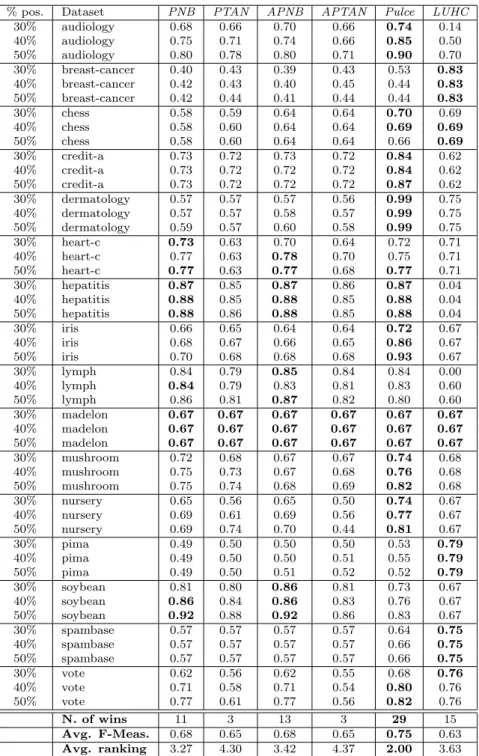
Table 3: F-Measure results over the 48 samples with k = 7 (χ2
F = 51.1875)
% pos. Dataset PNB PTAN APNB APTAN Pulce LUHC 30% audiology 0.68 0.66 0.70 0.66 0.74 0.14 40% audiology 0.75 0.71 0.74 0.66 0.85 0.50 50% audiology 0.80 0.78 0.80 0.71 0.90 0.70 30% breast-cancer 0.40 0.43 0.39 0.43 0.53 0.83 40% breast-cancer 0.42 0.43 0.40 0.45 0.44 0.83 50% breast-cancer 0.42 0.44 0.41 0.44 0.44 0.83 30% chess 0.58 0.59 0.64 0.64 0.70 0.69 40% chess 0.58 0.60 0.64 0.64 0.69 0.69 50% chess 0.58 0.60 0.64 0.64 0.66 0.69 30% credit-a 0.73 0.72 0.73 0.72 0.84 0.62 40% credit-a 0.73 0.72 0.72 0.72 0.84 0.62 50% credit-a 0.73 0.72 0.72 0.72 0.87 0.62 30% dermatology 0.57 0.57 0.57 0.56 0.99 0.75 40% dermatology 0.57 0.57 0.58 0.57 0.99 0.75 50% dermatology 0.59 0.57 0.60 0.58 0.99 0.75 30% heart-c 0.73 0.63 0.70 0.64 0.72 0.71 40% heart-c 0.77 0.63 0.78 0.70 0.75 0.71 50% heart-c 0.77 0.63 0.77 0.68 0.77 0.71 30% hepatitis 0.87 0.85 0.87 0.86 0.87 0.04 40% hepatitis 0.88 0.85 0.88 0.85 0.88 0.04 50% hepatitis 0.88 0.86 0.88 0.85 0.88 0.04 30% iris 0.66 0.65 0.64 0.64 0.72 0.67 40% iris 0.68 0.67 0.66 0.65 0.86 0.67 50% iris 0.70 0.68 0.68 0.68 0.93 0.67 30% lymph 0.84 0.79 0.85 0.84 0.84 0.00 40% lymph 0.84 0.79 0.83 0.81 0.83 0.60 50% lymph 0.86 0.81 0.87 0.82 0.80 0.60 30% madelon 0.67 0.67 0.67 0.67 0.67 0.67 40% madelon 0.67 0.67 0.67 0.67 0.67 0.67 50% madelon 0.67 0.67 0.67 0.67 0.67 0.67 30% mushroom 0.72 0.68 0.67 0.67 0.74 0.68 40% mushroom 0.75 0.73 0.67 0.68 0.76 0.68 50% mushroom 0.75 0.74 0.68 0.69 0.82 0.68 30% nursery 0.65 0.56 0.65 0.50 0.74 0.67 40% nursery 0.69 0.61 0.69 0.56 0.77 0.67 50% nursery 0.69 0.74 0.70 0.44 0.81 0.67 30% pima 0.49 0.50 0.50 0.50 0.53 0.79 40% pima 0.49 0.50 0.50 0.51 0.55 0.79 50% pima 0.49 0.50 0.51 0.52 0.52 0.79 30% soybean 0.81 0.80 0.86 0.81 0.73 0.67 40% soybean 0.86 0.84 0.86 0.83 0.76 0.67 50% soybean 0.92 0.88 0.92 0.86 0.83 0.67 30% spambase 0.57 0.57 0.57 0.57 0.64 0.75 40% spambase 0.57 0.57 0.57 0.57 0.66 0.75 50% spambase 0.57 0.57 0.57 0.57 0.66 0.75 30% vote 0.62 0.56 0.62 0.55 0.68 0.76 40% vote 0.71 0.58 0.71 0.54 0.80 0.76 50% vote 0.77 0.61 0.77 0.56 0.82 0.76 N. of wins 11 3 13 3 29 15 Avg. F-Meas. 0.68 0.65 0.68 0.65 0.75 0.63 Avg. ranking 3.27 4.30 3.42 4.37 2.00 3.63
task that involves a strategy game, where good and bad strategies often differ only because of few specific movements. This behavior clearly affects the neighborhood function adopted in our approach. This explains why low values of k give better results but it justifies also
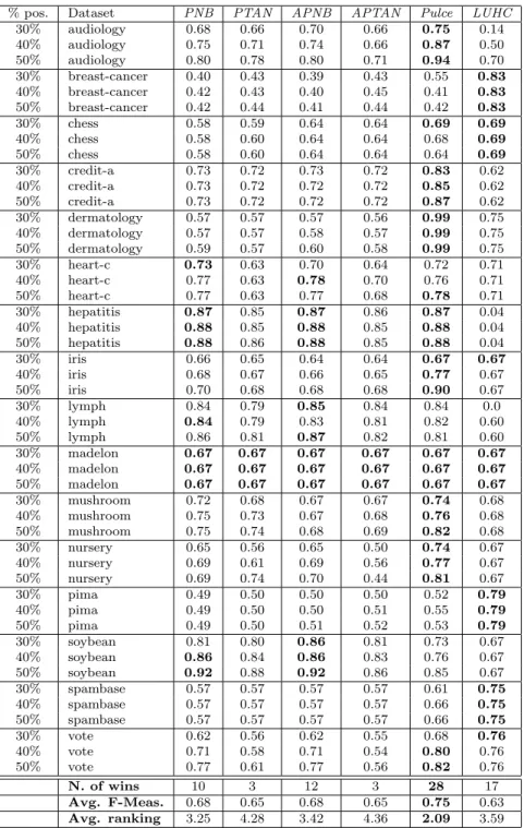
Table 4: F-Measure results over the 48 samples with k = 13 (χ2
F = 46.8155)
% pos. Dataset PNB PTAN APNB APTAN Pulce LUHC 30% audiology 0.68 0.66 0.70 0.66 0.75 0.14 40% audiology 0.75 0.71 0.74 0.66 0.87 0.50 50% audiology 0.80 0.78 0.80 0.71 0.94 0.70 30% breast-cancer 0.40 0.43 0.39 0.43 0.55 0.83 40% breast-cancer 0.42 0.43 0.40 0.45 0.41 0.83 50% breast-cancer 0.42 0.44 0.41 0.44 0.42 0.83 30% chess 0.58 0.59 0.64 0.64 0.69 0.69 40% chess 0.58 0.60 0.64 0.64 0.68 0.69 50% chess 0.58 0.60 0.64 0.64 0.64 0.69 30% credit-a 0.73 0.72 0.73 0.72 0.83 0.62 40% credit-a 0.73 0.72 0.72 0.72 0.85 0.62 50% credit-a 0.73 0.72 0.72 0.72 0.87 0.62 30% dermatology 0.57 0.57 0.57 0.56 0.99 0.75 40% dermatology 0.57 0.57 0.58 0.57 0.99 0.75 50% dermatology 0.59 0.57 0.60 0.58 0.99 0.75 30% heart-c 0.73 0.63 0.70 0.64 0.72 0.71 40% heart-c 0.77 0.63 0.78 0.70 0.76 0.71 50% heart-c 0.77 0.63 0.77 0.68 0.78 0.71 30% hepatitis 0.87 0.85 0.87 0.86 0.87 0.04 40% hepatitis 0.88 0.85 0.88 0.85 0.88 0.04 50% hepatitis 0.88 0.86 0.88 0.85 0.88 0.04 30% iris 0.66 0.65 0.64 0.64 0.67 0.67 40% iris 0.68 0.67 0.66 0.65 0.77 0.67 50% iris 0.70 0.68 0.68 0.68 0.90 0.67 30% lymph 0.84 0.79 0.85 0.84 0.84 0.0 40% lymph 0.84 0.79 0.83 0.81 0.82 0.60 50% lymph 0.86 0.81 0.87 0.82 0.81 0.60 30% madelon 0.67 0.67 0.67 0.67 0.67 0.67 40% madelon 0.67 0.67 0.67 0.67 0.67 0.67 50% madelon 0.67 0.67 0.67 0.67 0.67 0.67 30% mushroom 0.72 0.68 0.67 0.67 0.74 0.68 40% mushroom 0.75 0.73 0.67 0.68 0.76 0.68 50% mushroom 0.75 0.74 0.68 0.69 0.82 0.68 30% nursery 0.65 0.56 0.65 0.50 0.74 0.67 40% nursery 0.69 0.61 0.69 0.56 0.77 0.67 50% nursery 0.69 0.74 0.70 0.44 0.81 0.67 30% pima 0.49 0.50 0.50 0.50 0.52 0.79 40% pima 0.49 0.50 0.50 0.51 0.55 0.79 50% pima 0.49 0.50 0.51 0.52 0.53 0.79 30% soybean 0.81 0.80 0.86 0.81 0.73 0.67 40% soybean 0.86 0.84 0.86 0.83 0.76 0.67 50% soybean 0.92 0.88 0.92 0.86 0.85 0.67 30% spambase 0.57 0.57 0.57 0.57 0.61 0.75 40% spambase 0.57 0.57 0.57 0.57 0.66 0.75 50% spambase 0.57 0.57 0.57 0.57 0.66 0.75 30% vote 0.62 0.56 0.62 0.55 0.68 0.76 40% vote 0.71 0.58 0.71 0.54 0.80 0.76 50% vote 0.77 0.61 0.77 0.56 0.82 0.76 N. of wins 10 3 12 3 28 17 Avg. F-Meas. 0.68 0.65 0.68 0.65 0.75 0.63 Avg. ranking 3.25 4.28 3.42 4.36 2.09 3.59
the decrease of F-Measure for increasing percentage of positive examples. Notice also that learning good models in strategy games does not require a high quantity of examples, but that the few employed examples are of good quality.
0.5 0.55 0.6 0.65 0.7 0.75 0.8 0 5 10 15 20 25 30 35 F-measure k Eucl-30% Eucl-40% Eucl-50% KL-30% KL-40% KL-50%
Figure 3: Average F-Measure using the Euclidean distance and the Kullback-Leibler divergence.
Other factors that should be taken into account are related to under/overfitting phenom-ena. Our approach has two learning phases: the distance learning step and the k-NN step. Each of these steps suffers from typical (and sometimes unpredictable) classification biases. In some cases, too many positive examples may bias the classification task towards a major accuracy for the positive class. In some other cases, the problem is inverted. However, it can be noticed that when the number of positive examples is low (30%) our approach wins 9 times over 16 for k = {7, 11, 13} and 8 times over 16 for k = {1, 3}, for a win-ratio which is always higher than the overall win-ratio.
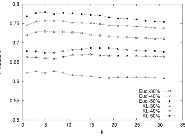
4.2. Impact of distance measure on Pulce
So far, we have considered the Euclidean distance as the standard metric to derive the distance model, as suggested by Ienco et al. [6]. However, alternative distance metrics may be employed as well. Here, we measure the impact of choosing another distance measure on classification results. In particular, we adopt the symmetric version of the Kullback-Leibler (KL) divergence [35], which measures the relative entropy between vectors representing probability distributions. In data mining, this measure is usually employed to quantify the divergence between two distributions defined over the same space. As such, it could be a good candidate metric for our framework. The Kullback-Leibler divergence is defined as
follows:
DKL(P ||Q) =
X
P (i) × logP (i) Q(i)
where P and Q are two different discrete distributions. In our framework, the Kullback-Liebler is used to quantify the difference between the distributions of two values yi and yj of
an attribute Y , for the given context C(Y), as described in Section 3.1. The KL divergence is then computed as follows:
DKL(yi||yj) = X X∈C(Y ) X xk∈X P (yi|xk) × log P (yi|xk) P (yj|xk)
This measure is asymmetrical in nature, i.e., DKL(yi||yj) 6= DKL(yj||yi), hence we employ a
symmetric version of the KL divergence: DsymKL(yi||yj) = D
sym
KL(yj||yi) =
DKL(yi||yj) + DKL(yj||yi)
2
In Figure 3 we report the results obtained by combining Pulce with the Euclidean distance and the symmetric KL divergence. The F-Measure is averaged on all datasets for a given percentage of positive examples. Thus, we plotted three curves corresponding to 30%, 40% and 50% of positive examples for each distance metric and increasing values of k. Figure 3 clearly shows that the Euclidean distance always performs better than the Kullback-Leibler divergence, in these experiments, no matter the percentage of positive examples.
A possible explanation for this phenomenon lies in the way the Euclidean distance is computed. The distance between two values yi and yj of the same attribute Y is bounded
and normalized to take values in the range [0, 1] (see Eq. 1). On the contrary, the DKLsym distance is unbounded (it ranges between 0 and infinite), and it cannot be easily normalized. This may introduce scale errors in the computation of the distance between two examples (see Eq. 3), leading to biased models for both positive class and reliable negative examples. 4.3. Statistical significance of the results
To asses the statistical quality of our approach we use the Friedman statistics and the Nemenyi test [36]. These techniques are usually employed to deal with the problem of evaluating the statistical relevance of results of different classifiers over multiple datasets. We briefly summarize the Friedman test:
1. the performance of each method on a certain issue (F-Measure, accuracy, etc) is de-termined on each data-set;
2. the methods are ranked for each dataset according to the results;
3. for each method, its average position Rj w.r.t. the datasets is computed;
4. finally, to compute the Friedman statistics the following formula is employed:
χ2F = 12N k(k + 1) " X j Rj− k(k + 1)2 4 #
where N is the number of datasets, k is the total number of methods and it is dis-tributed according to χ2F with k − 1 degrees of freedom.
We compare Pulce with all the competitors (PNB, APNB, PTAN, APTAN over 16 datasets with 3 different percentage of labeled positive examples, for a total of 48 datasets. In this statistical test the null hypothesis is that all the methods obtains similar perfor-mances, i.e., the χ2
F value is similar to the critical value for the chi-square distribution with
k − 1 degrees of freedom. At significance level of α = 0.001, the critical values of the chi-square is equal to 20.52. In our test we obtain values from 38.8869 to 51.1875 for the χ2F statistics (see captions of Tables 2 to 4), hence the null hypothesis of the Friedman test is comfortably rejected and we can now proceed with the post-hoc Nemenyi test. According to this test, the performance of two classifiers is significantly different if the corresponding average ranks differ by at least the critical difference:
CD = qα
r
k(k + 1) 6N
where α is the significance level and qα is the critical value for the two tailed Nemenyi test
[36] which is based on the Studentized range statistic divided by√2. Then, we compare the five methods at the critical value of q0.05 = 2.9677. The ranking table is shown on bottom
of Tables 2, 3 and 4. The critical difference is CD = 1.1333 (at significance level α = 0.05). We observe that, for k = 7 and k = 13, Pulce brings a statistically significant improvement w.r.t. all the four competitors, with an average rank of 2.00 and 2.09 respectively. For k = 1, Pulce’s average rank is also sensibly better than PNB’s, but, in these case, the difference is not statistically significant, even if only slightly. Notice also that the differences between the averaged version and the non averaged version of PNB and PTAN do not pass the Nemenyi test, i.e., these differences are not statistically significant.
4.4. Sensitivity analysis of the parameter k
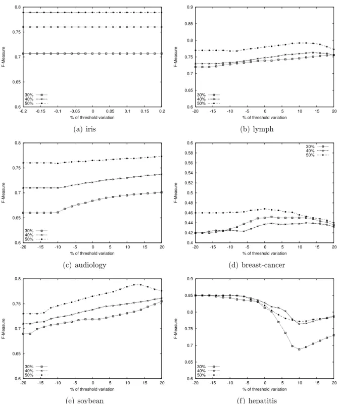
We now evaluate the sensitivity of Pulce to the variation of the parameter k. Due to space limitations, we can not show the complete set of results, hence we focus on the six datasets in which our method has the highest change in performance while varying the value of k: iris, soybean, audiology, breast-cancer, lymph and hepatitis. The results are reported in Figure 4. We observe that lymph and iris are the only datasets in which the highest variation is observed for the highest percentage of positive examples (50%) over which the classifier is learnt. For iris, one explanation for this apparently strange phenomenon is that, since the number of examples is low and the classes are not well separated, higher values of k are likely to introduce noise in the decision process of the k-NN classifier. This behavior, however, is observed for all percentages of positive examples, but is emphasized when the number of positive examples is large, since misclassified examples in the first step of Pulce have a major impact. Regarding lymph, with 30% and 40% of positive examples, we observe the classic learning curve: initially, it grows with k; then it remains stable; finally it starts to decrease slightly. With 50% of positive examples, the overall variation do not exceed 0.11.
0.6 0.65 0.7 0.75 0.8 0.85 0.9 0.95 1 0 5 10 15 20 25 30 35 F-Measure k 30% 40% 50% (a) iris 0.7 0.75 0.8 0.85 0.9 0 5 10 15 20 25 30 35 F-Measure k 30% 40% 50% (b) lymph 0.65 0.7 0.75 0.8 0.85 0.9 0.95 0 5 10 15 20 25 30 35 F-Measure k 30% 40% 50% (c) audiology 0.3 0.35 0.4 0.45 0.5 0.55 0.6 0 5 10 15 20 25 30 35 F-Measure k 30% 40% 50% (d) breast-cancer 0.64 0.66 0.68 0.7 0.72 0.74 0.76 0.78 0.8 0.82 0.84 0.86 0 5 10 15 20 25 30 35 F-Measure k 30% 40% 50% (e) soybean 0.76 0.78 0.8 0.82 0.84 0.86 0.88 0.9 0 5 10 15 20 25 30 35 F-Measure k 30% 40% 50% (f) hepatitis
Figure 4: Sensitivity analysis of parameter k for Pulce
In soybean we measure a variation of 0.10 for low percentage of positive examples (30%) while for higher percentage of positive examples the results are quite stable, as expected. For both breast-cancer and hepatitis the maximum variation is below 0.11 for the lowest
0.6 0.65 0.7 0.75 0.8 -0.2 -0.15 -0.1 -0.05 0 0.05 0.1 0.15 0.2 F-Measure % of threshold variation 30% 40% 50% (a) iris 0.6 0.65 0.7 0.75 0.8 0.85 0.9 -20 -15 -10 -5 0 5 10 15 20 F-Measure % of threshold variation 30% 40% 50% (b) lymph 0.6 0.65 0.7 0.75 0.8 -20 -15 -10 -5 0 5 10 15 20 F-Measure % of threshold variation 30% 40% 50% (c) audiology 0.4 0.42 0.44 0.46 0.48 0.5 0.52 0.54 0.56 0.58 0.6 -20 -15 -10 -5 0 5 10 15 20 F-Measure % of threshold variation 30% 40% 50% (d) breast-cancer 0.6 0.65 0.7 0.75 0.8 -20 -15 -10 -5 0 5 10 15 20 F-Measure % of threshold variation 30% 40% 50% (e) soybean 0.6 0.65 0.7 0.75 0.8 0.85 0.9 -20 -15 -10 -5 0 5 10 15 20 F-Measure % of threshold variation 30% 40% 50% (f) hepatitis
Figure 5: Assessment of the influence of the threshold in selecting reliable negative examples for Pulce
percentage of positive examples. The maximum variation observed in audiology, heart-c, and chess is around or less than 0.06, and it further decreases for mushroom, vote and pima (less than or equal to 0.02). This behavior is also observed when Pulce uses few
positive examples to learn the model. Finally, dermatology and nursery are stable: there is no remarkable variation in terms of F-Measure when the value of the parameter changes. In conclusion, Pulce’s results are reasonably stable w.r.t. the setting of parameter k: in most cases the maximum variation of the F-Measure is below 0.1, and it never exceeds 0.2. Furthermore, we notice that the highest F-measure values have been observed for small values of k (k < 15 in these experiments).
4.5. Shifting the threshold to asses the average-based criteria
In all the experiments we have reported above, the threshold for the selection of a set of reliable negative examples was set to the average distance computed between each pair of positive examples, as specified in Section 3.2. However, one can argue that this is not the optimal choice. Thus, in this section, we study the behavior of our classifier when the cut-off threshold varies between -20% and +20% of the average. We fix the value of k equal to 1, which is the most unstable setting for a k-NN classifier. This choice is justified by the fact that a worst case situation should stress any minimal change of the threshold value and, consequently, it should influence the results of Pulce maximally. To this purpose, we conduct these experiments on the six datasets reported in Section 4.4, due to the relative instability of their behavior. The results of this experiment are summarized in Figure 5. The six plots clearly show that there are no significant variations of the F-Measure except for heptatitis with 30% of positive labeled examples. This behavior can be explained by the low number of instances this dataset consists of and, in particular, by the small absolute number of positive labeled examples (only 9 data examples, as specified in Table 1). The most significant result that we can carry out from this experiment is that, even though the average value is not always the best choice, it represents a good trade-off if a user does not want to be concerned by complex parameter tuning. Otherwise, a classic training-validation-test model selection process can be employed to select an optimal cut-off threshold for each dataset.
5. Conclusion and future work
The presence of both positive and negative examples in training data is needed to build an efficient classifier, but this requirement is not always satisfied and in many domains only one class of samples is available. We have introduced Pulce, a distance based approach for Pos-itive Unlabeled learning (PU) in categorical data. Unlike the few existing approaches based on Naive Bayes, it takes into account data dependencies and learns a distance model from attribute relationships to train a k-NN-like classifier. Statistically significant classification results on real world datasets have validated our strategy, also comparing to state-of-the-art approaches. Finally, the sensibility analysis on the only required parameter and the study on variations of the proposed threshold for selecting a good example-set for the negative class and have shown that Pulce is stable and robust.
It is worth noting that, when the dataset contains numerical attributes, Pulce is not always the best choice: it requires a discretization step that is not straightforward. As shown in our experiments, a numerical approach is preferable in those cases. However,
compared to PU learning algorithms based on Naive Bayes, our method achieve better prediction performances.
As future work, we plan to investigate the extension of the binary PU learning task for categorical data to multiclass problems, and to embed our approach in an active-learning framework so as to involve users’ feedback along the learning phase.
References
[1] B. Calvo, N. L´opez-Bigas, S. J. Furney, P. Larra˜naga, J. A. Lozano, A partially supervised classification approach to dominant and recessive human disease gene prediction, Computer Methods and Programs in Biomedicine 85 (3) (2007) 229–237.
[2] H. Yu, J. Han, K. C.-C. Chang, Pebl: positive example based learning for web page classification using svm, in: Proceedings of KDD 2002, ACM, New York, NY, USA, Edmonton, Alberta, Canada, 2002, pp. 239–248.
[3] M. A. Zuluaga, D. Hush, E. J. F. D. Leyton, M. H. Hoyos, M. Orkisz, Learning from only positive and unlabeled data to detect lesions in vascular ct images, in: Proceedings of MICCAI 2011, Springer, Berlin, Toronto, Canada, 2011, pp. 9–16.
[4] F. D. Comit´e, F. Denis, R. Gilleron, F. Letouzey, Positive and unlabeled examples help learning, in: Proceedings of ALT 1999, Springer, Berlin, Tokyo, Japan, 1999, pp. 219–230.
[5] S. Boriah, V. Chandola, V. Kumar, Similarity measures for categorical data: A comparative evaluation, in: Proceedings of SDM 2008, SIAM, Philadelphia, PA, USA, Atlanta, GA, USA, 2008, pp. 243–254. [6] D. Ienco, R. G. Pensa, R. Meo, From context to distance: Learning dissimilarity for categorical data
clustering, Trans. in Knowledge Discovery from Data 6 (1) (2012) 1:1–1:25.
[7] L. Yu, H. Liu, Feature selection for high-dimensional data: A fast correlation-based filter solution, in: Proceedings of ICML 2003, AAAI, Palo Alto, CA, USA, Washington, DC, USA, 2003, pp. 856–863. [8] C. Elkan, K. Noto, Learning classifiers from only positive and unlabeled data, in: Proceedings of KDD
2008, ACM, New York, NY, USA, Las Vegas, Nevada, 2008, pp. 213–220.
[9] Y. Xiao, B. Liu, J. Yin, L. Cao, C. Zhang, Z. Hao, Similarity-based approach for positive and unlabeled learning, in: Proceedings of IJCAI 2011, AAAI, Palo Alto, CA, USA, Barcelona, Spain, 2011, pp. 1577– 1582.
[10] K. Zhou, G.-R. Xue, Q. Yang, Y. Yu, Learning with positive and unlabeled examples using topic-sensitive plsa, IEEE Trans. Knowl. Data Eng. 22 (1) (2010) 46–58.
[11] F. Mordelet, J. Vert, A bagging SVM to learn from positive and unlabeled examples, Pattern Recog-nition Letters 37 (2014) 201–209.
[12] J. Wu, X. Zhu, C. Zhang, Z. Cai, Multi-instance learning from positive and unlabeled bags, in: Pro-ceedings of PAKDD 2014, Springer, 2014, pp. 237–248.
[13] H. Li, Z. Chen, B. Liu, X. Wei, J. Shao, Spotting fake reviews via collective positive-unlabeled learning, in: Proceedings of IEEE ICDM 2014, IEEE, 2014, pp. 899–904.
[14] P. Yang, X. Li, H.-N. Chua, C.-K. Kwoh, S.-K. Ng, Ensemble positive unlabeled learning for disease gene identification, PLoS ONE 9 (5).
[15] B. Calvo, P. Larra˜naga, J. A. Lozano, Learning bayesian classifiers from positive and unlabeled exam-ples, Pattern Recognition Letters 28 (16) (2007) 2375–2384.
[16] N. Friedman, D. Geiger, M. Goldszmidt, Bayesian network classifiers, Machine Learning 29 (2-3) (1997) 131–163.
[17] J. He, Y. Zhang, X. Li, Y. Wang, Naive bayes classifier for positive unlabeled learning with uncertainty, in: Proceedings of SDM 2010, SIAM, Philadelphia, PA, USA, Columbus, Ohio, 2010, pp. 361–372. [18] Y. Zhao, X. Kong, P. S. Yu, Positive and unlabeled learning for graph classification, in: Proceedings
of ICDM 2011, IEEE, Los Alamitos, CA, USA, Vancouver, BC, Canada, 2011, pp. 962–971.
[19] Y. Shao, W. Chen, L. Liu, N. Deng, Laplacian unit-hyperplane learning from positive and unlabeled examples, Inf. Sci. 314 (2015) 152–168.
[20] B. Liu, W. S. Lee, P. S. Yu, X. Li, Partially supervised classification of text documents, in: Proceedings of ICML 2002, Morgan Kaufmann, Burlington, MA, USA, Sydney, Australia, 2002, pp. 387–394. [21] V. Chandola, A. Banerjee, V. Kumar, Anomaly detection: A survey, ACM Comput. Surv. 41 (3). [22] B. S. John, J. C. Platt, J. Shawe-taylor, A. J. Smola, R. C. Williamson, Estimating the support of a
high-dimensional distribution, Neural Computation 13 (1999) 2001.
[23] A. Blum, T. M. Mitchell, Combining labeled and unlabeled sata with co-training, in: Proceedings of COLT 1998, ACM, New York, NY, USA, Madison, WI, USA, 1998, pp. 92–100.
[24] M. C. du Plessis, M. Sugiyama, Semi-supervised learning of class balance under class-prior change by distribution matching, Neural Networks 50 (2014) 110–119.
[25] H. Gan, R. Huang, Z. Luo, Y. Fan, F. Gao”, Towards a probabilistic semi-supervised kernel minimum squared error algorithm, NeurocomputingAvailable online.
[26] S. Basu, A. Banerjee, R. J. Mooney, Semi-supervised clustering by seeding, in: Proceedings of ICML 2002, Morgan Kaufmann, Burlington, MA, USA, Sydney, Australia, 2002, pp. 27–34.
[27] I. Davidson, S. Ravi, The complexity of non-hierarchical clustering with instance and cluster level constraints, Data Mining and Knowledge Discovery 14 (2007) 25–61.
[28] M. Bilenko, S. Basu, R. J. Mooney, Integrating constraints and metric learning in semi-supervised clustering, in: Proceedings of ICML 2004, ACM, New York, NY, USA, Alberta, Canada, 2004, pp. 81–88.
[29] L. Ma, X. Yang, D. Tao, Person re-identification over camera networks using multi-task distance metric learning, IEEE Transactions on Image Processing 23 (8) (2014) 3656–3670.
[30] Y. Luo, T. Liu, D. Tao, C. Xu, Decomposition-based transfer distance metric learning for image clas-sification, IEEE Transactions on Image Processing 23 (9) (2014) 3789–3801.
[31] J. Yu, D. Tao, J. Li, J. Cheng, Semantic preserving distance metric learning and applications, Inf. Sci. 281 (2014) 674–686.
[32] M. Ring, F. Otto, M. Becker, T. Niebler, D. Landes, A. Hotho, Condist: A context-driven categorical distance measure, in: Proceedings of ECML PKDD 2015, Springer, 2015, pp. 251–266.
[33] R. J. Quinlan, C4.5: Programs for Machine Learning, Morgan Kaufmann Series in Machine Learning, Morgan Kaufmann, Burlington, MA, USA, 1993.
[34] C. J. Van Rijsbergen, Information Retrieval, 2nd Edition, Butterworth-Heinemann, Newton, MA, USA, 1979.
[35] S. Kullback, R. A. Leibler, On information and sufficiency, Annals of Mathematical Statistics 22 (1951) 49–86.
[36] J. Demsar, Statistical comparisons of classifiers over multiple data sets, Journal of Machine Learning Research 7 (2006) 1–30.