Analysis, Design, and Control for Robots in
Temperature-Restricted Environments
by
Ethan B Heller
B.S.M.E., Tufts University (2007)
MASSACHUSETTS INS1TIOi OF TEC OLOGY
4121:111
Submitted to the Department of Mechanical Engineering in partial fulfillment of the requirements for the degree of
Master of Science in Mechanical Engineering at the
MASSACHUSETTS INSTITUTE OF TECHNOLOGY
June 2013
©
Massachusetts Institute of Technology 2013. All rights reserved. A u th o r ... . . r ... ...Department of Mechanical Engineering May 10, 2013
Certified by ...
Kamal Youcef-Toumi Professor of Mechanical Engineering Thesis Supervisor
A ccepted by ... ...
David E. Hardt Professor of Mechanical Engineering Graduate Officer
Analysis, Design, and Control for Robots in
Temperature-Restricted Environments
by
Ethan B Heller
Submitted to the Department of Mechanical Engineering on May 10, 2013, in partial fulfillment of the
requirements for the degree of
Master of Science in Mechanical Engineering
Abstract
In this thesis, the problem of controlling the internal and external temperatures of a robot operating within a temperature-restricted environment was addressed. One example of a temperature-restricted environment is the interior of a holding tank for Liquefied Petroleum Gas (LPG), which is the focus of the analysis in this work, but not the only possible application. This gas is stored at sub-zero temperatures to maintain its liquidity, and any significant rise in temperature can cause the gas to vaporize, posing a safety hazard. The tank in which the gas is stored must be periodically inspected for defects. Using robot inspectors while the tank is in service would reduce the cost due to lost productivity during human inspection. A ther-mal management system (TMS) was designed to maintain the robot's electronics and components within operating limits, while preventing the external environment from increasing in temperature above safe levels. A detailed model of the system was con-structed for simulation, and the results indicate that the system performs as intended, but requires closed-loop control to maintain robot operation for extended periods of time. A control system based on system model linearization and model predictive control was implemented for the TMS. The results of the closed-loop simulations in-dicate that the control system enhances the operation of the TMS, maintaining robot operating temperatures for extended periods of time, while avoiding an unsafe rise in the temperature of the external environment.
Thesis Supervisor: Kamal Youcef-Toumi Title: Professor of Mechanical Engineering
Acknowledgments
I would first like to thank my advisor, Kamal Youcef-Toumi, and my labmates at
the Mechatronics Research Laboratory (MRL) for their help and support throughout the time it took to finish this thesis. Without the guidance of Prof. Youcef-Toumi and the other students in the MRL, none of this work would have been possible. In particular, my thanks go to Dimitris Chatzigeorgiou and Amith Somanath, who have been in the lab with me since the beginning, and have always provided help and advice when asked.
I also would like to thank GE Aviation, whose financial support and time
consid-eration was instrumental in my work here at MIT. I would specifically like to thank my patient managers and coworkers, who were understanding of my dual role.
The Qatar National Research Fund has generously supported the robotic inspec-tion project in progress both at MIT and Qatar University. I would also like to thank Prof. Uvais Qidwai of Qatar University for helping me understand their end of the project, and Tunde Yusuf of the RasGas Company for answering my questions about
LNG and LPG storage.
In the course of my studies I received help from many people, but there are a few who I would specifically like to thank. Dan Burns, a former member of the MRL, and Chris Laughman, both of the Mitsubishi Electric Research Laboratories, were always patient with my Dymola questions. John Batteh and Jesse Gohl of Modelon were even more patient with my questions on Dymola and everything Modelica, and invaluable in helping me make my simulation work. Finally, Leslie Regan in the graduate office forever has all the answers.
Last, and most importantly, I would like to thank my family. My ever-patient wife, Krystin, for putting up with the final few months of this endeavor, and my
parents, who kindly managed not to ask every day how the thesis was coming along. Without you, I would not have made it this far.
Contents
1 Introduction 15
1.1 M otivation . . . . 15
1.1.1 LPG and LNG Storage . . . . 15
1.1.2 Inspection of Gas Storage Tanks . . . . 16
1.1.3 Robotic Inspection . . . . 16
1.2 Background . . . . 18
1.2.1 Robot Design in Qatar . . . . 18
1.2.2 Need for Electronic Temperature Regulation . . . . 18
1.3 Prior W ork . . . . 19
1.3.1 Heat Storage for Electronic Cooling . . . . 19
1.3.2 Robots Operating in Space. . . . . 19
1.4 Thesis Structure and Scope . . . . 20
2 Design 23 2.1 Introduction . . . . 23
2.2 Design Concept . . . . 25
2.2.1 Restricted Waste Heat Rejection . . . . 25
2.2.2 System Design Objectives . . . . 27
2.2.3 Overview of the Thermal Management System . . . . 27
2.2.4 The Thermal Management System Used for Initial Analysis 28 2.3 A nalysis . . . . 29
2.3.1 Actuator Heat Generation . . . . 31
2.3.3 Thermoelectric Conversion . . . . 33
2.3.4 Thermal Rejection Convection . . . . 34
2.3.5 Thermal Resistor Model Results . . . . 35
2.3.6 Total System Power Generation . . . . 36
2.3.7 Thermal Storage Volume . . . . 37
2.4 Discussion . . . . 37
3 Modeling 39 3.1 Introduction . . . . 39
3.2 Modeling of the TM S components . . . . 41
3.2.1 Component Construction . . . . 41
3.2.2 Component Verification Testing . . . . 48
3.3 System Model . . . . 53 3.3.1 Assembly . . . . 54 3.3.2 Analysis . . . . 56 3.4 Discussion . . . . 59 4 Control 61 4.1 Introduction . . . . 61 4.1.1 Background . . . . 61 4.2 Design . . . . 65
4.2.1 Closed-Loop Control Construction . . . . 65
4.2.2 Model Modification for Control . . . . 67
4.2.3 Input and Output Choices . . . . 68
4.2.4 Choice of Linearized States . . . . 70
4.2.5 MPC Setup . . . . 70 4.3 Analysis . . . . 74 4.3.1 Controller Testing . . . . 74 4.3.2 Tuning Simulations . . . . 75 4.4 Results. . . . . 76 4.5 Discussion . . . . 79
5 Conclusions and Recommendations 5.1 Summ ary ...
5.2 Future Work ...
A Modelica Code and Graphical Models A.1 System Model ...
A.2 M otor Unit ... A.3 DC M otor ...
A.4 Heater ...
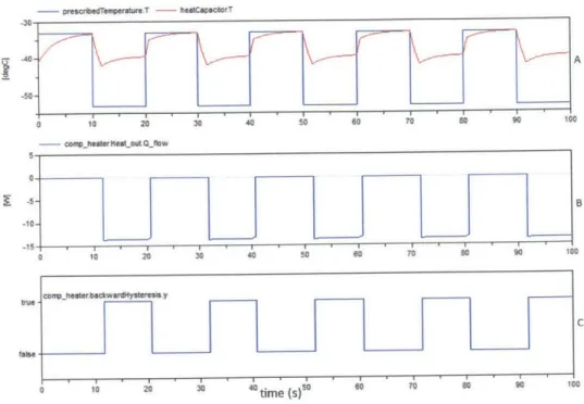
A.4.1 Backward Hysteresis . . . . .
A.5 Fluid Block . . . . A.6 TE Module . . . . A.7 HC-50 Medium . . . . A.8 PCM Block . . . . A.8.1 PCM Interior Unit . . . .
A.8.2 PCM Edge Unit . . . .
A.8.3 PCM Corner Unit ... A.9 External Convection ...
A.9.1 LPG Medium ...
B Modelica Verification Testing and Simulink
B.1 Verification Testing . . . .
B.2 Simulink and Dymola Comparison Tests . . . .
C Matlab Code
D Closed-Loop Simulation Test Results
83 . . . . 83 . . . . 86 87 . . . . 87 97 100 103 105 106 109 110 114 119 121 123 125 129 133 133 138 145 153 Comparison Testing
List of Figures
1-1 Neptune II... .. ... 17
2-1 Comparison of the components . . . . 26
2-2 Layout of analyzed Thermal Management System . . . . 29
2-3 Thermal resistance model without PCM energy storage . . . . 30
3-1 Fluid block thermal resistance data-fit results . . . . 42
3-2 Fluid block m odel . . . . 43
3-3 Dymola model of PCM block . . . . 45
3-4 Fluid block verification test results . . . . 49
3-5 TE module verification test model . . . . 50
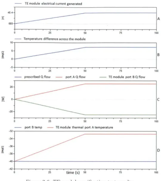
3-6 TE module verification test results . . . . 51
3-7 PCM block verification test results . . . . 52
3-8 External convection verification test results . . . . 53
3-9 Heater verification test results . . . . 54
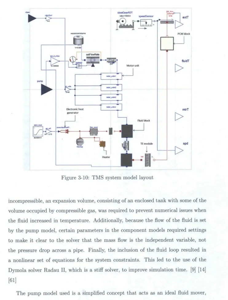
3-10 TMS system model layout . . . . 55
3-11 System responses for three levels of fluid flow . . . . 58
3-12 Dymola results to a trapezoidal velocity input . . . . 59
4-1 Illustrations of two time window implementations . . . . 67
4-2 Comparison of the heat flow to the PCM block or ambient . . . . 68 4-3 Simulation velocity results with poorly-shaped output reference values 73 4-4 Dymola motor temperature results to a trapezoidal velocity input . 74
4-6 Closed-loop velocity results . . . .
4-7 Closed-loop output results comparison: measured vs. linearized . . . 4-8 Closed-loop motor temperature comparison: measured vs. linearized .
4-9 Closed-loop velocity comparison: measured vs. linearized . . . .
4-10 Velocity results for the end of the simulation . . . .
4-11 External temperature results for the end of the simulation . . . .
Dymola graphical model of the TMS system . .
Dymola graphical model of the motor unit . . .
Dymola graphical model of the DC motor . . .
Dymola graphical model of the heater . . . .
Dymola graphical model of the fluid block . . .
Dymola graphical model of the PCM block . . .
Dymola graphical model of external convection . Fluid block verification test model . . . . PCM block verification test model . . . .
External convection verification test model . . .
Heater verification test model . . . .
. . . . 88 . . . . 97 . . . . 100 . . . . 103 . . . . 106 . . . . 114 . . . . 125 . . . . 134 . . . . 135 . . . . 136 . . . . 137
B-5 Dymola model of the TMS system used for Dymola/Simulink compar-ison tests . . . .
B-6 Simulink model of the TMS system used for Dymola/Simulink com-parison tests . . . .
B-7 Dymola results for the external heat flow . . . .
B-8 Simulink results for the external heat flow . . . .
B-9 Dymola results for the PCM average temperature . . . . B-10 Simulink results for the PCM average temperature . . . .
B-11 Dymola results for the fluid block heat flows . . . .
B-12 Simulink results for the fluid block heat flows . . . . B-13 Dymola results for the system temperatures . . . .
B-14 Simulink results for the system temperatures . . . .
77 78 79 80 80 81 A-i A-2 A-3 A-4 A-5 A-6 A-7 B-i B-2 B-3 B-4 138 139 140 140 141 141 142 142 143 143
D-1 Closed-loop calculated control commands . . . . 153
D-2 Closed-loop output predictions of the MPC . . . . 154
Chapter 1
Introduction
The components of a robot generate waste heat during operation, which must be removed or those components may cease to work properly. In most cases, that waste heat is rejected to the ambient environment, but in some cases the environment cannot tolerate the rejection of waste heat. It is for these circumstances that a Thermal Management System (TMS) is proposed. This system incorporates several additional components in the robot construction, in order to safely transport the heat away from the generating components, store the heat, and reject the heat to the environment. The proposed design was modeled in Dymola and simulated in MATLAB/Simulink with both open-loop and a proposed closed-loop control. These simulations illustrate the usefulness of the TMS for robot operation in a refrigerated environment, but use of this system is not limited to those cases.
1.1
Motivation
1.1.1
LPG and LNG Storage
Once retrieved and processed, Liquefied Petroleum Gas (LPG) and Liquefied Natural Gas (LNG) are often stored in large, above-ground tanks. The interiors of these tanks are kept refrigerated, in order to keep the gasses in their liquid state. When stored at atmospheric pressure, LPG is chilled to -45 'C and kept below -42 'C to prevent
vaporization. The typical storage temperature of LNG is even colder at -162 'C, and it must be kept below -158 'C to avoid vaporization. [45]
[58]
The storage tanks typically have diameters of roughly 100 m and heights of 50 m. [43] These tanks can be constructed in a number of styles. The most common tank style is double-walled, with insulation sandwiched between two steel walls. Regular inspection of the tank walls is necessary to ensure that the steel does not contain any flaws, such as corrosion, cracks, or weld defects. Inspection specifications and intervals for refrigerated tanks vary depending on what type of liquefied gas is being stored. [44] [3]
1.1.2
Inspection of Gas Storage Tanks
The outer surface of the tank can be inspected for defects while the tank is in operation with no loss of productivity. Interruption in the operation of a tank represents a very large loss of productivity, so tank inspection is ideally performed with the tank still in service. However, the current inspection process for the inside of a liquefied gas holding tank is to drain the tank of all the gas, bring the interior temperature up to human-survivable levels, and to manually inspect the interior surface. This entire maintenance cycle, including re-refrigerating the tank and refilling it with gas, can take up to eight months, at the cost of approximately $10 million per day in lost productivity. [58] It is therefore clear that a solution for in-operation inspection is immensely beneficial. One such solution is the use of robotic inspectors.
1.1.3
Robotic Inspection
There are great advantages to operating robots as inspectors inside liquefied gas hold-ing tanks versus ushold-ing human inspectors. These robots can perform necessary inspec-tions on the tanks without the environmental restricinspec-tions that human inspectors have. This allows the robots to perform the inspections while the tank is still in service, saving significant money for the tank operator during the inspection. Additionally, removing the need to place a person within an enclosed hazardous environment
signif-icantly increases operational safety, regardless of whether the inspection is performed with the tank in or out of operation.
Figure 1-1: Neptune II used with permission from http://www.frc.ri.cmu.edu/ -hagen/samplers/figures/neptuneon-rustyplate .gif
Robots for inspection of petrochemical holding tanks have existed as a commercial option for many years. There are many examples of robots that inspect the outer walls of holding tanks using either magnetic treads or wheels, or suction-tipped limbs to climb the sides of the tanks, such as those presented in [37], [38], [50], [51], [60],
and [25]. Fewer robots inspect the tank interiors. Two examples of current in-tank inspection robots-for products stored at room temperature-are the Neptune system and the TechCorr On-Stream Tank Inspection System (OTIS). The Neptune system is capable of performing floor and wall inspections to American Petroleum Institute (API) standard 653. The robot uses both vision and ultrasonic sensors to gather inspection data. The Neptune II robot is shown in Fig. 1-1. [52] Similarly, OTIS also performs API 653 inspections on the floor of storage tanks. TechCorr operates
OTIS on a commercial basis, with several systems in operation. As of March 2011, OTIS has inspected over 175 tanks. [56] However, these two robots are still limited
1.2
Background
1.2.1
Robot Design in Qatar
One project in progress to design a robotic inspector for use in refrigerated liquefied gas holding tanks is out of Qatar University. Their design incorporates safety features such as brushless motors to avoid any potential sparks that can be ignition sources, and an insulated compartment for the robot's electronics. Two types of sensors are incorporated into the design: magnetic flux leakage sensors and visual sensors. The current choice for the magnetic flux leakage sensor is the Silverwing Handscan. Using these sensors in combination allows the robot to identify defects in the interior wall of the holding tank. [6]
1.2.2
Need for Electronic Temperature Regulation
Though the electronics in the Qatar robot are insulated against the refrigerated en-vironment, there are no active or passive controls over the temperature of those electronics. As the inspection takes place, the electronics will generate heat, and when kept inside an insulated compartment, will eventually saturate their environ-ment with this heat. Once the compartenviron-ment is saturated with the electronics' waste heat, the internal temperature of the electronics will increase, leading to overheating, and shutting down the robot. Some method must be employed to remove the waste heat from the electronics in order to maintain proper robot operation during inspec-tion. This method must also be actively monitored to ensure that the waste heat leaving the robot does not pose a safety risk in the ambient environment of liquefied gas.
1.3
Prior Work
1.3.1
Heat Storage for Electronic Cooling
One method of removing the waste heat from the electronics without rejecting that heat to the ambient environment is to store most of the heat energy. Phase-change materials are already used commercially to store thermal energy when that energy cannot be dissipated. One application of this use is to maintain the temperature of electronics operating in heated ambient environments. As described in [41], a heat sink incorporating heat storage in the form of phase-change material (PCM) is utilized in firefighting as a method of keeping infrared cameras cool within the environment of a building fire. In this case, the PCM absorbs the heat generated by the camera when the ambient temperature is above the temperature of the electronics, increasing the running time of the camera before overheating.
Other works, such as
[55]
and [16], address the design of PCM-filled heat sinks as a method of maintaining temperatures of electronics in the face of peak usage, where the design of a cooling system capable of dissipating the peak heat generation does not fit with the usage of the electronics (such as in mobile devices). Both of these works specifically focus on increasing the operating time of electronics before overheating, and mention the need to include heat spreaders in the PCM to evenly distribute the heat through the PCM due to the poor thermal conductivity of the material.1.3.2 Robots Operating in Space
Although the use of PCM can help ensure that the electronics do not overheat, being too cold for operation is also a concern. When operating in very cold environments, the electronics must be maintained above their lower operating temperature limit. Most of the prior work in the heating of electronics for applications in cold environ-ments relates to the operation of robotic craft in space. The most obvious parallel to draw is to the robotic rovers used in the Mars missions. These rovers (including the
latest, Curiosity) house their main electronics in a Warm Electronics Box (WEB). [33] [34] This box provides an insulated, temperature-controlled environment for the rover's non-hardened electronics. NASA provides some of the heating to the WEB through electronic heaters, and the remaining heating requirements are met by ra-dioisotope heating units, which are used to conserve electrical energy. [35] The WEBs of the Mars rovers are insulated to reduce the heating requirements. The insulation used in the WEBs is based on silica aerogel, a very lightweight material with extremely low thermal conductivity. [36]
1.4
Thesis Structure and Scope
The body of this thesis is structured into three chapters, each of which defines a distinct stage in the development of the Thermal Management System. The chapters contain background information on the concepts used in that particular stage of the TMS development and relevant discussion.
Design of the TMS This chapter details the development of the TMS concept and outlines the components that could be included in the configuration of the TMS. Descriptions of the individual TMS components and their purposes are given. The initial calculations that were performed show that the proposed concept will work with commercially-available components.
Modeling of the TMS This chapter describes the detailed modeling of one con-figuration of the proposed TMS using the Modelica modeling language. The system model is constructed of both standard and custom component models. Verification testing confirmed that the component models behave as expected to simple inputs. Several open-loop control simulations show that the TMS system behaves as intended, and does indeed maintain robot component temperatures within operational levels for a longer time than without the TMS. However, closed-loop control is necessary to maintain robot operation for extended periods of time.
Control of the TMS This chapter covers the development of the closed-loop con-trol for the TMS in the MATLAB/Simulink environment. The Modelica model is exported to Simulink, where MATLAB functions are used to create a control system for the TMS to ensure that system constraints are not violated during operation, even for long durations.
Chapter 2
Design
This chapter proposes one design of a thermal management system for robots to meet the challenges detailed in Chapter 1. Initial calculations show that this concept can be implemented for an ambient environment of refrigerated LPG, maintaining the components of the robot within operating temperatures and limiting the surrounding temperature rise to safe values.
2.1
Introduction
Though robots are commonly deployed in a wide array of settings, one environment that has not received much attention yet is one in which the robot surface temperature cannot exceed a certain value. These environments include surroundings where safety or an operational constraints limit the release of waste energy, such as areas that are refrigerated. Examples of cold environments that robots currently operate in are space or on other planets, and underwater. However, venting waste heat into these environments is not typically an issue, unlike the interior environment of a liquefied gas holding tank, where the product inside must be maintained at very cold temperatures to prevent vaporization and avoid safety hazards.
Typical waste heat rejection The waste heat generated by a robot's systems
op-erating environment. For a robot opop-erating on land in a thermally-unconstrained environment, rejection of generated waste heat is typically performed by either
pas-sive or active convection of the heat to the surrounding air inside the robot chassis or conduction through the component housing. The air within the chassis is then circu-lated with the surrounding ambient environment. Rejection of waste heat underwater substitutes the circulation of air for convection of heat from the chassis or housing to the ambient environment. When the ambient environment is a vacuum, radiators are deployed alongside active heat collection systems that reject waste heat into space. In all of these conditions, the rejection of waste heat is dependent on the requirements of the robot components, and the amount of heat rejected or rejection rate is not considered. With the additional constraint of the environmental requirements, the heat rejection system of the robot must incorporate components and controls that provide sufficient component cooling, and govern the amount of heat rejected from the robot.
Robots operating in cold environments typically control the temperature of their electronics. For the robot to operate in a very cold environment, the on-board elec-tronics must be heated to operating temperatures. Typical elecelec-tronics operate at temperatures warmer than -40 'C, and electronics that operate in colder environ-ments are either too costly for commercial use or still being researched.
[49]
[19]Most of the prior work in heating electronics for this application is related to the operation of robotic craft in space applications. The closest parallel to draw is to the robotic rovers used in the Mars missions, which house their electronics in an insulated warm electronics box. This WEB must also maintain the electronics below the upper operating limits and incorporate methods for venting the. excess heat when necessary.
[35]
Liquid cooling designs The use of fluid loops as a carrier for waste thermal energy
is currently employed in many existing systems. Computers and cars are two exam-ples of everyday items that may use liquid cooling loops to maintain proper system temperatures. These systems can be obtained commercially with numerous options
available. Most of the commercial offerings are not designed to work at freezing tem-peratures, however, and are not made of suitable materials for this application. [62]
2.2
Design Concept
The thermal management system proposed actively removes the generated waste heat from the robot sub-systems and safely vents some of that energy into the ambient environment. The removal of waste heat in this situation requires additional sub-systems in the robot compared to a typical robot. These sub-sub-systems must maintain the operational temperatures of the robot components and safely reject the excess heat into the surrounding environment. These new systems require active controls to optimize robot performance and maintain operational safety. The concept detailed in this work is based on current commercial technologies for thermal management, implemented for an LPG environment.
2.2.1
Restricted Waste Heat Rejection
Robots operating within thermally-constrained environments require additional spe-cial sub-systems for proper waste heat management. Figure 2-1 shows a comparison of the general components in a typical robot and the components of a robot us-ing the proposed thermal management system. This system incorporates a thermal carrier that collects and transports components' waste heat to a thermal rejection de-vice, which interfaces with the surrounding environment. Optionally, the system may contain heaters that maintain components within operational temperatures, ther-mal storage devices that can absorb the waste heat instead of rejecting it to the environment, thermo-electric (TE) conversion devices that convert the temperature differential between two components of the thermal management system into usable electric energy, and insulation covering the robot. All of these components may be singular, plural, or distributed within the robot.
Typical Robot Components
Electronics
Power Supply
Actuators
-
Sensors
-A
Proposed Robot Components
Thermal Rejection
(Thermal Storage
Actuators
Sensors
Heaters
TE Conversion
Thermal Insulation
BFigure 2-1: Comparison of the components in a typical robot (A) and the proposed system (B)
2.2.2 System Design Objectives
Operating in cold and hazardous environments also requires control of the tempera-ture of the robot's electronics. In conjunction with the electrical heaters, the on-board electronics create their own waste heat, reducing the load on the heaters once robot operation is underway. Since this waste heat will be trapped within the insulated WEB, a method of maintaining the electronics' temperatures is required to ensure that operational temperatures are not exceeded. In order to safely reject the heat as needed to the surrounding environment (comprised of LPG for this implementation) a controllable device for venting will be incorporated in or on the robot. This heat sink is fed the collected waste heat of the robot's electronics, sensors, and actuators. The components are insulated against the ambient environment to prevent unsafe heat loss.
Robots operating in cold and hazardous environments must not only control the temperature of their electronics, but also the temperature of their external surfaces. To prevent uncontrolled heat loss and reduce the amount of heating of the electronics required, the interior of the WEB is insulated against the environment. The insulation covering the proposed WEB, and the other electronics on the robot not housed in the WEB, is based on silica aerogel, the same insulation used on the WEBs of the
Mars rovers. [36] This insulation provides a very high thermal resistance versus
density ratio, compared with other commercially available insulations. In addition, several commercial variants of silica-based aerogel insulation can be obtained in easily-installed sheets. [21] [48] [57]
2.2.3 Overview of the Thermal Management System
The thermal management system may contain multiple zones to obtain optimal sys-tem performance. The syssys-tem may have to maintain different robot sub-syssys-tems at different maximum temperatures to satisfy the sub-system operating conditions. Each of these zones contains an independent thermal carrier system, but may share any of the other thermal management system components. Additionally, each of the
optional components of the system need not be incorporated into all zones.
Using multiple zones for components of different thermal requirements allows for
optimal tuning of the thermal management system. Allowing some sub-systems to retain more heat reduces the amount of heat rejection necessary. Each of the zones in the thermal management system may be controlled separately, with a supervisory control that maintains communication with each zone and enforces the environmen-tal constraints, or all zones may be controlled together. The control systems set and
maintain the thermal management system effort on the active sub-systems, and po-tentially reduce the robot sub-system operation levels below the commanded levels to maintain acceptable thermal conditions. The supervisory controller uses a perfor-mance index based on the error between the robot component command levels and actual operating levels, and the effort expended by the thermal management system to maintain acceptable thermal conditions.
2.2.4
The Thermal Management System Used for Initial
Anal-ysis
The proposed thermal management system, analyzed as a feasibility study in this chapter, considers only one zone in the system. The analyzed system was based on the design of current liquid-coolers, but optimized for cold environments. This thermal management system, shown in Fig. 2-2, spans the robots actuators, sensors, and other electronics, and is designed to function in a similar manner to liquid-coolers used in high-performance desktop computers. The primary difference between this system and a commercial solution for a desktop computer is the use of materials that are suited to the temperature range required in this application. Because this system operates mainly within the freezing range of most standard liquid-cooling solutions, a different type of fluid is required. After comparison of several potential heat-transfer
fluids that maintain liquidity to -50 0C, Dynalene@HC-50 was chosen as the liquid for
use in the initial calculations.
[23]
Care was taken in choosing the pump and tubing components for material compatibility with both the HC-50 and the cold environment.heat sink /PCMV hybrid
TE device
fluid pump(s)
sensor(s)
system electronics
actuator with insulation covering
Figure 2-2: Layout of analyzed Thermal Management System
For weight and ease of installation, a polymer is chosen as the preferable material for the tubing. Several polymers exhibit glass transition temperatures within the desired range and are compatible with HC-50, such as ethylene propylene rubber. [1] [24]
If the robot's systems at full power consumption can produce more heat waste than
is safe to discharge at once, some heat must be absorbed. The heat sink attached to the thermal management system may be designed to absorb some of the waste heat. Thermal waste absorption can be accomplished via the inclusion of Phase-Change
Material (PCM) within the heat sink. As the energy from the thermal transfer fluid is passed into the heat sink, the PCM will absorb the energy, and release a portion to the heat sink fins. The preferential absorption of energy into the PCM is accomplished via the internal interfaces between the PCM, the heat sink base, and the heat sink fins. With this method, the rate of energy transfer to the ambient environment will not exceed safety limits.
2.3
Analysis
The thermal analysis presented for the thermal management system is an initial numerical assessment of one potential system to evaluate its suitability for full sim-ulation. The system is constructed primarily of commercially-available components, utilizing the thermal management system detailed in this paper. This initial study is based on the power consumed by a typical actuator system and by the robot
elec-~~~~powersupypoieenrytt actuator , hc odcsteha hog h
L Tactuator
Ractuator mountmn
TCF bWW, Rfluid bkok cold
lfluid block hot T e
THF R t heatsink
Tamb
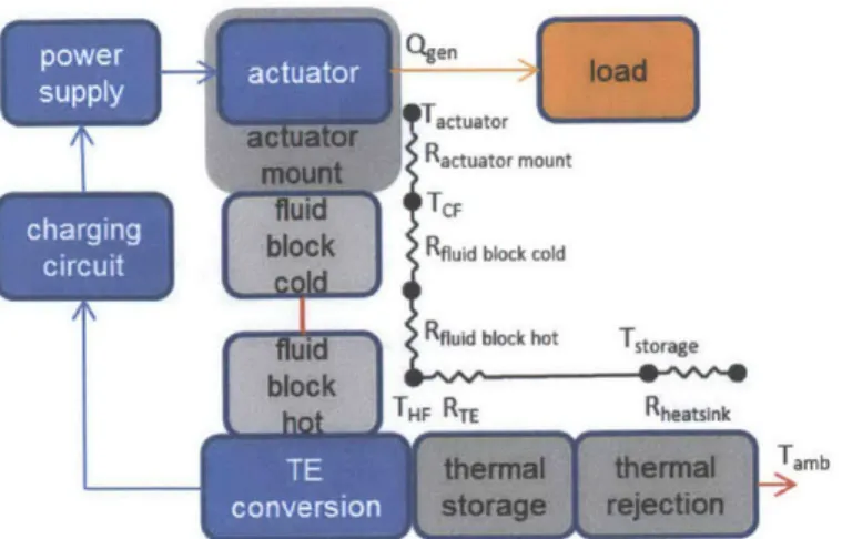
Figure 2-3: Thermal resistance model without PCM energy storage
tronics. Figure 2-3 shows a representation of a possible implementation of the robot components that are involved in the generation or transportation of waste heat. The power supply provides energy to the actuator, which conducts the heat through the actuator mount to the fluid blocks of the thermal management system. The TE con-version device feeds electrical energy back to the power supply, and reduces the heat load that is either stored or directly rejected to ambient.
A simple thermal-resistance model of the system was developed and analyzed. Figure 2-3 shows the thermal resistance model used overlaid on the representation of the thermal management system proposed. The model analyzed considers only the heat transfer from the actuator through the actuator mount and two heat-transfer fluid blocks, which is released to the ambient environment via a finned heat sink, with a TE conversion module placed between the second fluid block and the heat sink. This model makes the following assumptions:
" The external ambient environment is at temperature Te.,t.
" The thermal properties of the thermal transfer fluid in the system are invariant. " The thermal transfer fluid experiences no heat loss or gain within the system
except at the specific heat transfer blocks. * The fluid pump does not require cooling. " The properties of the TE module are constant.
e All system components have zero thermal capacity.
Additionally, the following conditions of the system were chosen:
" The robot actuators are motors generating waste heat.
" The heat sink is Lh, per side, cubed, with N fins of Nth thickness.
For this analysis, the ambient environment is chosen to be liquid propane maintained at -45 'C with properties found in
[4],
and the thermal transfer fluid properties are based on is Dynalene HC-50 fluid at -40 0C. Additionally, the actuators are assumedto generate 25W each, and the physical properties of the heat sink are as follows: Lh,
= 10 cm, N 10, and N = 5 mm.
2.3.1
Actuator Heat Generation
The robot actuator considered in this analysis is a motor that would typically provide power to the drivetrain. Though typical robots contain as least two of these actuators, only a single motor was considered for this analysis for simplicity, with the energy gen-erated by multiple motors addressed later. This type of actuator can generate waste heat from both its electronics and the electrical resistance from the motor windings. To avoid any potential sparks that could present a hazard in the working environment, a brushless motor was chosen for use in the design of the robot. The motor chosen to represent this typical drive motor is a Maxon electronically-commutated brushless DC motor, number 283872. As indicated in [5], the normal operating ambient tempera-ture range of this motor is between -40 and 100 0C; therefore very little supplemental
heating will be required when operating within LPG, though significant heating will be necessary to reach operating temperature when inspecting LNG tanks. The tem-perature of the single actuator is determined based on its power consumption, which is determined from the torque generated, using calculations from [26]. The actuator's temperature is calculated from the torque generated, which determines power draw. The actuator's power consumption is calculated in Equ. (2.1) and used in Equ. (2.2)
to determine the actuator temperature:
T2
P = 2* R (2.1)
kt
Tmotor = P * Rth + Tmount (2.2)
where P is the electric power dissipated by the motor, T is the motor torque, Re
is the electrical resistance of the motor windings, kt is the motor torque constant, Rth is the thermal resistance of the motor windings, and Tmotor and Tmount are the motor and motor mount temperatures, respectively. The values of Re and kt are
temperature-dependent.
The heat generated from the actuator passes through the actuator mount, which is connected thermally to a fluid block. The capacitance of the mount is not considered, but the thermal resistance of the mount is modeled and added to the total system's thermal resistance.
2.3.2
Thermal Transfer Fluid
The thermal transfer fluid carries the waste heat generated by the actuator to the heat sink via the fluid blocks. After conduction of the heat through the actuator mount, the heat is conducted through the fluid block and convected to the thermal transfer fluid. The mass transport of the heat transfer fluid in this proposed system is assumed to take place within insulated tubing, and as such, no heat transfer from the fluid is calculated in-between the two fluid blocks.
At each fluid block (connected to the actuator mount and the TE module) the heat convection to the thermal transfer fluid is calculated based on parameters for forced flow within a square cross-section. This type of convection has a constant value for the Nusselt number, NUFB, and the value of the heat transfer coefficient, hFB, is
calculated as
NUFB * kFB
hFB- D(23
Dh
conduc-tion of the fluid. The Nusselt number used in Equ. (2.3) is a dimensionless parameter that represents a ratio of the convective to conductive heat transfer at a surface based on the Prandtl number (Pr), another dimensionless parameter, which is a ratio of fluid momentum and thermal diffusivity. [30] The convection is then modeled as a thermal resistance, which is counted in the system's total thermal resistance. [27]
2.3.3
Thermoelectric Conversion
The heat passing from the fluid block through the TE conversion module results in electricity generation from the Seebeck effect, converting some of the waste heat back into usable power. Equation (2.4) shows the power generation in the TE module as a function of the temperature difference between the two sides of the device. Equation
(2.5) defines the temperature difference, relating it to the thermal resistance of the TE module. [63]
I a2 AT 2
QTE = -( 'e ) (2.4)
2 Reiec,total
AT = (THF - THS) = (in - QTE)RTE (2.5)
In these equations, QTE is the rate of heat flow removed from the system by the generation of electrical power in the TE module, ase is the Seebeck coefficient of the
TE module, AT is the temperature difference over the TE module, and
Qin
is the rateof heat flow entering the TE module. Reiec,total is the total electrical resistance of the
TE module (module electrical resistance plus load-with the load resistance taken as
equal to the module resistance). RTE is the thermal resistance of the TE module,
THF is the hot fluid block temperature, and THS is the heat sink temperature. For this analysis ase is set to 2.2*10-4 V/K, and Reiec,totai is chosen to be 2Q.
Equations (2.4) and (2.5) are solved iteratively with the equations in Section 2.3.4 to determine the value for QTE. The resulting power generated by the TE module, equal to the power removed from the thermal circuit, is very small, 0.55 P W. This small power output from the TE module is due to a calculated dT across the module of only 6.8 'C. The calculated value of RTE is counted in the system's total thermal resistance.
2.3.4
Thermal Rejection Convection
Thermal rejection in this system is performed by a finned heat sink. To simplify the initial analysis, a thermal storage component is not included in the model. Thus, free
convection from a standard finned heat sink is modeled for the thermal rejection of the system. To model the energy flow, the value of the heat transfer coefficient, h, for free convection at the heat sink is calculated in Equ. (2.6). This calculation requires
determining Nu in Equ. (2.7), which in turn is solved from the calculation of the Rayleigh number from fluid and system properties in Equ. (2.8).
The following is a list of the notation used in Equs. (2.6)-(2.8): oz is thermal
diffusivity of LPG, 3 is the volumetric expansion coefficient of LPG, V is the kinematic viscosity of LPG, g is the acceleration due to gravity, k is the thermal conduction of
LPG, Pr is the Prandtl number, and T, is the surface temperature.
Na * k h = (2.6) L 0.670Ra/4 Nu = 0.68 + 0.492 )9/16)4/9 (2.7) Ra = g(Ts - Text)L3 (2.8)
The Rayleigh number, used in Equ. (2.7), is another dimensionless parameter. The
Rayleigh number is the ratio of the buoyancy and viscous forces in the fluid multiplied
by the Prandtl number. [28] Solving Equs. (2.6)-(2.8) for the free convection from
the heat sink to the liquid propane requires iterating though the value of T, for the heat sink fins.
The thermal resistance of the heat sink, R, is calculated in Equ. (2.9), based on
the overall surface efficiency in Equ. (2.10). The fin surface efficiency used in Equ. (2.10) is calculated in Equ. (2.11), based on the parameter m calculated in Equ. (2.12), which is determined using the value of the heat transfer coefficient in Equ.
(2.6).
R (2.9)
NAf ro= *(1 -)f (2.10) At tan m * L2.11)
m
*c h * Pf m = h *Af (2.12) M k * A,The following is a list of the notation used in Equs. (2.9)-(2.12): Ac is the cross-sectional area of the fin, Af is the surface area of the fin, At is the total surface area of the fin, L is the length of the fin, L, is the fin length plus half the fin thickness, and Pf is the perimeter of the fin.
These equations thermally connect the cold side of the TE module to the ambient environment through the thermal resistance in Equ. (2.9), which is added to the system's total thermal resistance.
2.3.5
Thermal Resistor Model Results
From the thermal resistance analysis, a final value for the temperature rise of the actuator can be determined, in addition to the required thermal transfer fluid mass flow. The analysis assumes that the amount of heat generated from the actuator, minus the power recovered by the TE module, is safe to vent to the environment and is completely rejected to ambient. The rejected heat can used with the total system thermal resistance, RTotaI, to calculate the total temperature difference, ATyS,
between ambient and the actuator. The value of RTotal is obtained by summing each component's thermal resistance, like that calculated by Equ. (2.9).
ATsys = (Tmotor - Text) = (Qgen - QTE)RTotal (2.13)
The generation of waste heat by the operation of the actuator results in an actuator temperature within operational limits. The temperature difference in Equ. (2.13) is calculated to be 65 'C. The resulting actuator temperature of 20 0C is within the actuators' operating temperature range. [5] [29]
[31]
For the single actuator waste heat elimination, the heat-transfer fluid will have to be pumped at a rate under 0.3mL/s to maintain the heat transfer rate assumed. [23]
2.3.6
Total System Power Generation
The above analysis considers only a single source of heat generation, but robots will have many sub-systems that all generate heat. The previous calculations assume that the thermal management system can safely dispose of all the waste heat generated
by the system, otherwise, some energy must be stored for venting when the
ther-mal outputs of the sub-systems are reduced, and capacity remains in the ambient environment to absorb the stored energy.
The total robot power consumption is determined based on the following condi-tions for total energy production:
" Four actuators generating a total of 100 W waste heat, peak. " PCM is paraffin technical grade 5913 (C13-24).
" The robot electronics (not including actuators and sensors) generate 13 W waste
heat, peak.
" The robot-mounted non-destructive testing sensor generates 33.6 W waste heat,
peak.
The electronics' waste heat generation is based on the waste power output of an Intel® AtomTM D525 processor. [32] The sensor waste heat generation is based on the power consumption of the Silverwing Handscan magnetic flux leakage sensor. [54] The total generated power is calculated to be 146.6 W.
The thermal power capacity of the LPG environment is calculated and compared to amount of thermal power generated by the system. To determine the amount power the LPG can absorb without vaporizing, a mass of liquid propane corresponding to a volume 1 mm thick, the width of the heat sink, and as long as the distance traveled by the robot in 1 s (assumed to be 0.25 m) is considered as the heat absorbing medium.
Limiting the rise in LPG temperature by 4 'C, this mass can safely absorb 130.8
obtained from [41), while the robot's systems produce 146.6 J (based on the total generated power of 146.6 W for 1 second). The difference of 15.8 J per second must therefore be stored within the heat sink.
2.3.7
Thermal Storage Volume
In systems that generate more waste heat than can be safely absorbed by the environ-ment, the excess energy must be stored on-board the robot. One method of storing thermal energy is to utilize a PCM to absorb the energy, which requires a relatively small volume of material versus using a single-phase material storage solution.
Based on the properties of solid paraffin (C13-24)
[151,
a heat sink with 10 cm 3 ofPCM could absorb the 15.8 J per second excess heat generation for 82.5 seconds before it is completely melted. The energy stored by the PCM, denoted by E, is shown in Equ. (2.14), where c is the heat capacity of the PCM, ATPcm is the temperature difference between the PCM and the heat source, V is the volume of PCM, and A is the latent heat of fusion of the PCM. [41]
E = pV * (cATPCM + A) (2.14)
2.4
Discussion
A possible thermal management system for robots in temperature-restricted
envi-ronments is detailed that utilizes thermally-conductive liquid to cool multiple robot electronic components, and incorporates a control system to limit the thermal output of the system. Initial calculations for an ambient environment of LPG, where the thermal output must be regulated to ensure safe operation, show that the system can be implemented with commercially-available components. This system is shown to be able to maintain a single actuator at 20 'C within an ambient environment of LPG with a required thermal fluid flow rate of only 0.3 mL/s. For four actuators, some storage of the waste heat generated will be required to avoid an unsafe increase in the LPG temperature. A heat sink with 10 cm3 of solid paraffin was calculated
to be able to absorb the excess peak waste heat output of the robot for 82.5 seconds before being completely melted. The next chapter will present a detailed model of the proposed system.
Chapter 3
Modeling
This chapter details the construction and simulation for a detailed model of one possible implementation of the proposed TMS. The modeling was performed in the software package Dymola, which uses the Modelica language for multi-physics mod-eling, and simulates models numerically. The TMS system model was constructed from standard, built-in component models whenever possible, but some of the TMS components required custom models to represent the physics of the component. The behavior of each component model and the system model was simulated with open-loop inputs, and the models were verified to respond as expected. Open-open-loop simula-tions of representative inspection scenarios show that closed-loop control is required to maintain all system states within operating limits.
3.1
Introduction
Background of Dymola and Modelica Development of the modeling language
Modelica was first started in 1996 by Hilding Elmqvist, seeking to apply the principles of object-oriented programming to modeling multi-physics systems. This concept al-lows for the drop-in re-use of models within a system, simplifying the user-generated code. The first industrial use of Modelica occurred in 2000. In the same year, the Modelica Association was founded.
[47]
Since then, the language has been devel-oped and improved on, and currently is in version 3.2. [2] The language is releasedopen-source, and many different open-source and commercial programs exist that use Modelica for modeling.
Native usage of Modelica is via text-based object-oriented programming, but the language allows for annotations that define icons, which can be used in a graphical interface. Additionally, the Modelica language does not assign causality during model definition, but rather assigns relationships between states of different components. These relationships are later assigned causality for numerical simulation at the time of model compilation. Modelica describes the physics and interactions of the components as sets of Differential Algebraic Equations (DAEs). The constitutive equations of all objects are described in these DAEs, which are used to evaluate system state values during the model compilation into assigned, causal code.
Dymola is a commercial program offered by Dassault Systemes, AB, that uses the open-source Modelica language to model systems, and that provides several different solvers to simulate those models. In addition to the Modelica Standard Library
(MSL), which contains pre-constructed models of components for electrical, magnetic,
mechanical, and thermal-fluidic systems, as well as pre-defined mediums for use in the thermal-fluidic systems, Dymola is compatible with any Modelica-based library. Several open-source and commercial libraries exist for specialized modeling purposes, such as the Modelon Liquid Cooling library used later in this work, which focuses on the modeling of fluids to which heat is being added or subtracted, often in closed loops. Additionally, Dymola offers the user a graphical interface for interacting with Modelica, allowing a model to be constructed via the connection of icons representing system components. In the definition of a model, system states need not be assigned
a strict start value for simulation. In the case of a linear system, these values are calculated at the time of simulation, but for nonlinear systems, Dymola employs an iterative method to determine the start values for the system states. In many component models, these initial states can be constrained through the use of options. This capability becomes very important in this work during the control of the TMS model.
simplified the design of the model to a great extent. Specifically, for components such as the TE module, determination of the driving side for heat flow was not required at the time of model construction. This is compared to using causal modeling languages, which would have required additional determinations of heat flow characteristics of the system for model construction.
3.2
Modeling of the TMS components
The TMS component models were constructed largely from existing MSL models, modified only by setting parameters and the connections between models to form a sub-system. Several of the TMS components could not be realized by standard MSL models however, and for these components custom models were constructed with the appropriate physics. The Modelica definition of the models used in this work can be found in Appendix A.
3.2.1 Component Construction
Five component models were created to assemble the TMS model. These models represent the system motors as the heat generators, which are connected to the fluid blocks, allowing for heat transfer between the motors and the heat-transfer fluid. A PCM block is modeled as the heat storage device, a TE module as the heat recovery device, and there is a model of heat convection to ambient over a moving plate, representing the heat release device. With the exception of the motors, each of these main components required some sort of custom modeling.
Fluid blocks This component model was designed to model the behavior of a Priatherm PT Zed 1518 with Dynalene HC-50 flowing through it. [23] [8] To create this model (and the fluid loop in the system), the HC-50 medium first had to be defined in the Modelica language. Since HC-50 starts to phase transition into a vapor at 118 'C
[17],
the medium was limited in scope and execution between -50 and 110thermal fluid when it is in a two-phase state. (It is also worth noting that the thermal carrying capability of HC-50 drops significantly when it has become a vapor.)
10-6 s 2 s temperature (C)
flow (1pm)
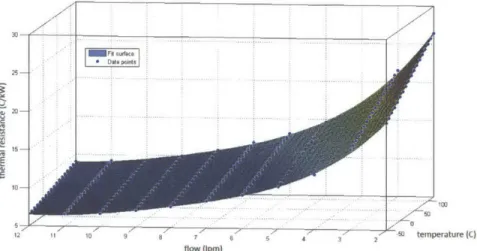
Figure 3-1: Fluid block thermal resistance data-fit results
The second custom component of the fluid block model set the value of the thermal resistance (Rth) of the fluid block from the liquid to the surface. This component acted as a function of two variables, and output the Rth of the PT Zed 1518 based on the medium temperature and volumetric flow rate. The function used to calculate
Rth was based on data from the PT Zed 1518 data sheet for the thermal resistance of the block using a 50% volumetric mix of water and Ethylene Glycol at 40 0C.
[8]
From this Rth versus volumetric flow data, a grid of Rth values over volumetric flow and temperature was determined for HIC-5O using interpolations based on the difference in properties between the two media and the change in medium properties with temperature. This grid of Rth values was then imported into Matlab, where a polynomial function was used to fit a surface over the data within the operating points of the fluid. The resulting surface-fit function matches the calculated Rth data, as shown in Fig. 3-1, with enough accuracy to use in the Modelica model of the fluid block, representing the value of the thermal resistance of the fluid block from the fluid to its surface. The plot shows that the thermal resistance of the fluid is highest when there is low flow and the fluid temperature is high. This result aligns with the expectation that increased fluid flow results in more heat being convected to the fluidbecause of higher fluid velocities, and thus an increased convection coefficient. portal
thermal conductance calculation
thermal mass of fluid block
temperatureSensor
degC
TA 0
volume flow meter
Figure 3-2: Fluid block model
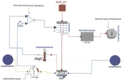
The model of the fluid block, shown in Fig. 3-2, consists of a fluid pipe with heat transfer to the convection model, where the Rth calculated is used to determine the
heat flow to a thermal port. This thermal port is where the fluid block connects to another component model in the system. Finally, the thermal capacitance of the aluminum wall of the fluid block is taken into account in the model with a capacitance based on the mass of the block itself. Though some sources, such as [22], have constructed fluid blocks for cooling electronics using element-based models similar to the construction of the PCM block in Fig. 3-3, this simulation is more concerned with the absolute temperature of the fluid in the block rather than the temperature distribution, and thus this model uses only a single element for representing the flow and heating of the fluid within the block.
Thermo-electric modules The TE modules are modeled in Dymola using only
the constitutive equations for the thermo-electric generation, and no sub-models. These equations calculate the heat flow across the module from equations based on the generation of electricity within the module:
dQhoIt = Se * Thot * I + K * dT - - 2 R, (3.1) 2
1
dQcold = Se *Tol I+K*dT+ - * I 2 * Re (3.2)
2
I = Se(Tot -TcId) (3.3)
2Re
where K is the thermal conductance of each module half, Se is the Seebeck coeffi-cient of the thermocouples, and I is the current across the TE module. dT is the temperature difference across the module and Re is the electrical resistance of the TE
module, and the electrical resistance of the load on the module. [63] These equations make the following two assumptions: the properties of the TE module are constant in
time, where typically the value of Se is dependent on temperature, and the electrical resistance of the load is equal to the electrical resistance of the TE module itself, to provide the most efficient power generation. Additionally, the thermal conductance of the module is assumed to be a known constant. The properties for the TE module
used in this simulation come from the properties of the TE module simulated in [63]. Because the electrical supply of the robot in the TMS simulation is not modeled, the power generated from the TE module is also not modeled, though the generated current can be observed.
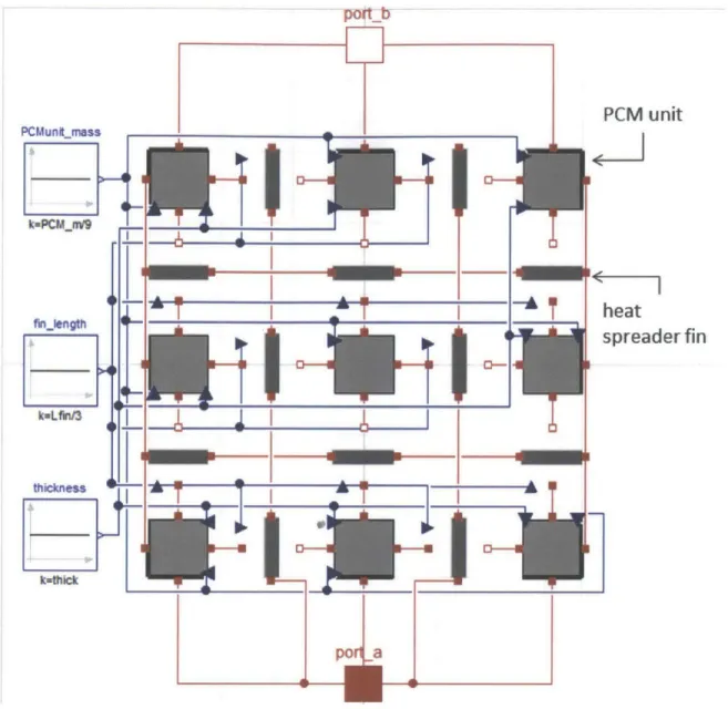
PCM block The construction of the PCM block, the thermal storage in the system,
is most complex of the TMS component constructions. The PCM block is modeled as a two-dimensional array of PCM masses enclosed in an aluminum case, with aluminum fins spaced between the masses to act as heat spreaders. The model is shown in Fig.
3-3. Three types of PCM mass models were constructed for the component, for each
of the center, edges, and corners of the block. All three of these models have the core PCM mass in common, which is a modified version of the MSL thermal capacitance. The PCM capacitance has a variable value dependent on the temperature of the mass in order to emulate the effects of the latent heat of melting for the PCM. Previous work in [20] has shown that using an arc tangent function to represent the heat capacity of the PCM allows for a series expansion calculation of the value of the thermal capacitance, which yields accurate and computationally quick results. Other
port~b I PCM unit I-A M I-I I-I A
-I
.1. II
0-I imm~I
-A T7~~i
A,
I---- I I I A
7,-
I
heat spreader finFigure 3-3: Dymola model of PCM block
load without increased accuracy. The thermal capacitance of the PCM mass is thus modeled as:
htransitin + C
(3.4)
C
i(((T - Ttransition)CMR)2+ 1) (
where c, is the effective heat capacity, htransition is the latent heat of melting, T is current PCM mass temperature, Transition is the temperature of melting, CMR is the melting range coefficient, used to adjust the width of the melting range, and cp* is the sensible heat of the PCM. The temperatures are assumed to be in Kelvin. The thermal capacitance is surrounded by standard thermal resistance blocks to mimic
PCMunit mass k-PCM-m/9 k~LfhO thicnes k=tick 7T