An approach to planning and control of stochastic network flows

(1)

An Approach to Planning and Control of Stochastic Network Flows

by

Michael J. Paskowitz

Submitted to the Department of Electrical Engineering and Computer Science in Partial Fulfillment of the Requirements for the Degrees of

Bachelor of Science in Computer Science and Engineering

and Master of Engineering in Electrical Engineering and Computer Science at the Massachusetts Institute of Technology

,May 22, 2000

D 2000 Michael J Paskowitz. Altrights reserved.

The author hereby grants to M.I.T. permission to reproduce and distribute publicly paper and electronic copies of this thesis

and to grant others the right to do so.

Author

Department of Electrical Engineering and Computer Science May 22, 2000 Approved by Certified by

(

Accepted by. Chairman SteVhan E. 1i The Charles Stark Draper Laboratory, Inc.

Technical Supervisor

C'ynthia Barnhart Codirector, MIT Operations Research Center ThqKue risor

Arthur C. Smith

, Department Committee on Graduate Theses

MASSACHUSETS NTJuiN ! OF TECHNOLOGY

(2)

An Approach to Planning and Control of Stochastic Network Flows

by

Michael J. Paskowitz

Submitted to the

Department of Electrical Engineering and Computer Science

May 22, 2000

In Partial Fulfillment of the Requirements for the Degrees of Bachelor of Science in Computer Science and Engineering

and Master of Engineering in Electrical Engineering and Computer Science

ABSTRACT

Large scale real-time planning and execution of complex flow-based networks requires careful modeling and analysis. These real-time systems often need to be modeled for an indefinite amount of time, and are often faced with unpredictable, stochastic changes to the system over time. Real-time planning must be done progressively, adapting to change as or after it occurs. Implemented plans must strive to be as efficient as possible while conforming to network demand and resource constraints. This thesis presents an approach to the planning and execution of stochastic real-time network flow problems. The approach taken is to apply linear programming, a deterministic network solution technique, to a stochastic real-time network flow problem with an unbounded time horizon by solving finite sections of the entire problem, one by one, over time. The approach is analyzed using a case study problem in the domain of military logistics planning. The analyses offer insight into more general application of this approach to other real-time network flow problems.

Technical Supervisor: Stephan E. Kolitz The Charles Stark Draper Laboratory, Inc.

(3)

Acknowledgements

There are many individuals to whom I owe my deepest thanks and gratitude for their contributions to my thesis research.

First and foremost, I would like to thank Dr. Stephan Kolitz of Draper Laboratory and Professor Cynthia Barnhart of MIT for their constant guidance and support. Even with the many obligations of their own work, they both found the time and effort over the past year to help drive my research to completion. I could not have come this far without their collective experience, technical vision, and sage advice.

I am grateful to the Charles Stark Draper Laboratory for its commitment to education,

and for funding my MIT tuition.

Thanks also go to Bill, my Draper buddy, for his countless contributions to my work experience.

My parents, Irv and Jean, deserve my highest praise for their faith and support over the

past year, and the 22 that preceded it.

Finally, now and forever, I would like to express my grateful appreciation and love to my fianc6e Maria. Her motivation and encouragement have kept me working hard on this project, and have shown me that there really is a light at the end of the tunnel.

This thesis was prepared at The Charles Stark Draper Laboratory, Inc, Company Sponsored Research: Real-Time Large-Scale Optimization,

2036.

Publication of this thesis does not constitute approval by Draper or the Institute of Technology of the findings or conclusions contained herein. solely for the exchange and stimulation of ideas.

under Internal IR&D Project Massachusetts It is published Michael J. Paskowitz 22 May 2000

(4)

(5)

1. Introduction

A flow-based network is a weighted, directed graph with two sets of specially

designated nodes, the sources and the sinks, and a capacity function that maps edges to

positive real numbers. The edges of the graph are generally directed from source to sink,

and the weights represent the maximum amount of flow that can travel along each edge

[2]. Flow refers to one or more commodities, either as discrete elements or continuous

streams, that are present at the sources and travel to the sinks through the various edges

of the network. Water flows from reservoirs to kitchen sinks by way of pipes and water

pressure tanks. Airlines transport millions of passengers a year between numerous cities

around the world using a limited number of planes. Distributors supply goods from

warehouses to customers through various distribution channels. Inherent in each of these

and many other flow-based networks is a problem that has to be solved: on which edges

should the commodities travel so that each sink receives its required amount of the

commodity in the most timely and efficient manner possible? Such problems are known

generally as minimum-cost network flow problems [ 1].

Parameters are values assigned to nodes and edges of a graph. For network flow

problems parameters include the amount of supply at each source, the flow capacity of

each edge, and the demand at each destination or sink. Many networks also have

constraints specific to their particular problems. A constraint is a logical relation between

(8)

flow problem impose restrictions on flow beyond those stated by edge capacities. Values

associated with constraints on a network flow are also considered parameters of that

network. In the case of the airlines, each plane must have a flight crew and some number

of flight attendants, and must be fueled, cleaned, and loaded to some capacity before it

can take off. The overall schedule of flights is also subject to weather conditions, other

traffic at the airports, and maintenance requirements.

Certain types of network flow problems need only be solved rarely. Infrastructure

networks like water and electric utilities are determined when the network is built and

essentially fixed for a long period of time. A flow-based network with fixed edges and

edge weights (i.e., that do not change over time) is considered a static network [1]. In

designing a water supply network the problem is to determine the best way to supply

sufficient water to each destination while minimizing the total number of pipes used and

minimizing the costs of installation and maintenance. It might be twice as cheap to lay

pipes aboveground rather than bury them in the ground, but they might then require four

times as much maintenance. Once decisions like this have been made and the network is

in place, flow proceeds as intended and the problem is considered solved. When a link

fails, it is typically rebuilt to match its preexisting condition and maintain the same

network structure.

This approach works for some systems, but not all network flow problems are

static. A network flow problem that airlines must solve involves the routing of passengers

(9)

flight schedule for the airline's fleet. In practice, such schedules face ever-changing

network conditions that must be taken into account. Planes can have mechanical

difficulties or fail to depart on time. Pilots and flight attendants may call in sick and need

to be replaced. An airport may close in the middle of a snowstorm. Because the

conditions of an airline network change over time, any one solution to its scheduling

network flow problem is only viable for a short period of time. Thus the problem must

be re-solved regularly, and the flow of passengers redirected (to a different plane, or a

later time) to maintain a feasible solution. Flow-based networks with parameters that

change over time are called time-expanded or dynamic networks [1].

Another example of a dynamic network flow problem is supply-chain logistics

planning. This problem is found in various forms in many commercial and military

situations. The network sources are supply warehouses of one or more goods. The sinks

are any destinations, perhaps retail stores, construction sites, or fielded forces, which

need a recurring supply of the goods stored at the warehouses. The network flow

problem involves how to most efficiently transport goods from warehouses to

destinations with demand [1]. The military commonly deals with this type of problem.

In times of war, the military must supply its fighting forces with food, medical supplies,

and munitions. This problem is dynamic since both supply network conditions and

demand requirements can change over time.

Small network flow problems can be solved either by inspection or some limited

(10)

discussed, could have an extremely large number of possible solutions and hundreds of

thousands of decisions that need to be made. These decisions are complicated by perhaps

thousands of constraints that must all be considered and satisfied together. Any set of

decisions that satisfies all constraints on the network is afeasible solution to the network

flow problem. A feasible solution may often be found by heuristic guidelines, but it is

unlikely that heuristic methods will yield an optimal solution [6]. The optimal solution to

these problems is the one that both satisfies all the constraints and minimizes the costs

involved in executing the solution. Execution is the process of physically implementing

the theoretically planned solution and actually moving flow from sources to destinations.

Finding the optimal solution to a large network flow problem can be extremely

difficult, requiring a significant amount of computing resources and a great deal of time.

Established linear programming methods exist for formulating and optimally solving

these problems. The formulation involves setting down the decisions to be made in the

problem as collections of variables, defining parameters with single values, codifying

constraints as equations in those variables and values, and describing the objective as a

function to be minimized (or maximized). With such a formulation a computer can

manipulate the millions of resulting possibilities through proven rigorous methods and

produce an optimal solution [7].

Often these problems require integer values for some or all of their decisions.

UPS, for example, cannot fly 1.7 planes between Boston and Dallas. Mixed Integer

(11)

variables must be integer. The general problem of solving a mixed integer programming

problem optimally is NP-complete [7]. Thus no polynomial-time algorithm for solving a

generic mixed integer problem has yet been found [5]. Typical real-world scheduling,

routing, and transportation problems are very large, and so are very expensive in time and

resources to solve as a whole. One approach to take is to decompose large problems into

smaller ones, and solve those directly [9]. The benefits to this approach are speed of

solution and economy of computing resources, but often the objective value suffers from

the artificial boundaries imposed on the problem. Applying a provably optimal algorithm

to the whole problem, rather than isolated pieces of it, is guaranteed to produce at least as

good a solution, and probably a better one.

For the dynamic flow networks discussed thus far, the dynamic parameters of the

network, those that change over time, can be either deterministic or stochastic in nature.

Deterministic parameters change over time according to some function, which can either

be known or unknown to network planners. If all other network parameters (including

time) are held constant, the deterministic network parameters will also remain constant.

Stochastic network parameters change according to random event incidence - their

values are determined by a probabilistic function. Even with all static and deterministic

parameters held constant, the actual realization of a stochastic network parameter cannot

be perfectly predicted. Many network flow problems that model real-world systems have

stochastic characteristics. Transportation networks face weather delays and personnel

availability issues. Logistics and supply networks might have to accommodate

(12)

processes. The future generally cannot be known, only predicted. Network parameters

are expected to change, but the exact time and magnitude of such changes can only be

estimated. Systems that model flow-based networks and include random events and

parameter values that affect the final solution are called stochastic network flows.

Solving stochastic network flow problems involves not only routing flow from source to

destination, but also reacting to events that randomly occur and adjusting the solution to

compensate.

Because stochastic network parameters change unpredictably, one way to attack

network flow problems involving stochastic parameters is to solve them repeatedly over

time. The frequency of re-solution depends on the impact of random events on the

existing solution, which varies from problem to problem. Significant changes to network

parameters may require immediate replanning to avoid a drastic increase in total cost.

Stochastic network flows that result from airline flight plans and the execution of

logistics supply plans are real-time systems. A real-time system in this context is a

dynamic network flow that models actual events and reacts to changes in network

parameters as (or soon after) they occur. These systems are often volatile, as unexpected

events can transpire with little or no warning, and require frequent replanning to maintain

feasible solutions. The time duration of many real-time planning systems is unbounded,

either because there is no desired end to the system being modeled or because the exact

(13)

week or next year, but indefinitely, with recurring (and possibly shifting) demand over

time.

It is undesirable to plan deterministically over even an approximation of an

unbounded time horizon because the conditions of the network will probably change. So

the question becomes, how can mathematical programming techniques be used in a

stochastic real-time system for planning and execution over an unbounded time horizon?

It is the goal of this thesis to explore an approach to planning and execution of

stochastic real-time network flow problems. The approach taken is to apply linear

programming, a deterministic network solution technique, to a stochastic real-time

network flow problem with an unbounded time horizon by solving finite sections of the

entire problem, one by one, over time. The solution to a single finite section is called a

partial plan, because it plans the movement of flow for only part of the problem's time

horizon. We therefore refer to our approach as the partial planning approach.

Figure 1 presents some common ways to classify network flow problems,

including static vs. dynamic networks, deterministic vs. stochastic events and parameters,

and fixed vs. unbounded planning time horizons. We are interested in planning a

dynamic real-time system with stochastic network events, and will focus our analyses on

a military logistics planning problem. This problem has the characteristics we are

interested in investigating, and a linear programming model is readily available for

(14)

Static Networks:

Water and Electricity supply networks Dynamic Networks:

Deterministic Network Parameters

Stochastic Network Events

Fixed duration Construction site Single season Cruise

planning horizon materials supply Line ship schedule

Unbounded Goods delivery network Airline flight plans,

planning horizon to meet known and Military logistics recurring demand planning and execution Figure 1: Classification of Common Network Flow Problems

The military logistics planning problem includes the movement of ammunition from interior United States depots to coastal US ports. Stochastic events encountered in

this problem include transportation delays, the loss of network links between depots and ports, and sudden shifts in demand if there is a crisis or contingency. Using this problem as a case study, our goal is to gain insight into the best way to apply the partial planning approach to real-time network flow problems under various network conditions. In addition, we shall examine the benefits of timely and accurate network parameter estimation and the effects of stochastic events on plans already in place.

(15)

detailed explanation of the objectives of the thesis. Chapter 3 explores the details of

solving linear programs and running scenario analyses, and provides specific

implementation details for the solution methods used in this thesis. In Chapter 4, the

specifics of the military logistics planning problem are explained, and the problem

formulation is given. Various scenario analyses and relevant results are presents in

Chapter 5. Chapters 6 and 7 provide a summary of the research accomplished,

(16)

2. Intent and Objectives

The intent of this thesis is to determine which methods for applying the partial

planning approach produce the least expensive solutions to various classifications of

network flow problems. In this chapter we define three objectives which will assist in

making that determination. Each objective involves the evaluation of various forms of

the partial planning approach as applied to specific network flow situations. We begin by

describing the details of the partial planning approach and the forms in which it can be

applied to various types of network flow problems.

2.1 The Partial Planning Approach

The partial planning approach to solving a network flow problem with an

unbounded time horizon involves the decomposition of the horizon into finite sections,

which are then solved using deterministic linear programming techniques. The finite

solutions, referred to in Chapter 1 as partial plans, are executed serially over time to route

flow in the original, unbounded network flow problem.

Several aspects of the approach can be varied to produce more efficient, or

cost-effective, solutions to the same problem. More efficient solutions are relatively less

expensive than other solutions. Variable aspects include the length of time for each

(17)

between partial plans. Each aspect is described in greater detail in the following sections

of this chapter. Specifying a value for every one of these aspects defines a particular

variant of the approach. By applying a number of variants to the same network flow

problem, we will be able to determine the variant that produces the least expensive

solution. The procedure for applying a specific variant is described in Section 3.4.

Within each variant, the values for partial plan length and replan delay time are consistent

- every partial plan is the same length, and each are combined with the same degree of

continuity.

Once a partial plan begins execution, the flow determined by that plan cannot be changed. Events that occur during a partial plan's execution cannot be compensated for

by that plan. The effects of such events on network parameters have to be incorporated

into the generation of the next partial plan.

2.2 Partial Plan Length Effects

The first objective of this thesis is to determine the effects of the length of each

partial plan on the cost of a given network flow problem's solution. To isolate the effects

of plan length from those of the other aspects mentioned in Section 2.1, the variants of

the approach used for this determination all use a periodic replanning schedule and ignore

plan continuity. Periodic replanning indicates that every partial plan finishes execution

before a new partial plan begins. Replans thus occur at regular time intervals over the

(18)

To fully appreciate the effect partial plan length has on the solution, we need to consider two major types of network flow problems: deterministic and stochastic. We

expect that for deterministic networks, longer partial plan variants will produce

consistently lower cost solutions because each partial plan is able to optimize over a

longer period of time. In stochastic networks, however, the longer partial plan variants

will likely be adversely affected by each partial plan's inability to compensate for change.

Section 5.1 details the application of various partial plan lengths to both

deterministic and stochastic networks. The results found there provide insight into the

relationships between partial plan length and solution cost.

2.3 Network Parameter Forecasting and Assessment

Deterministic solution methods like linear programming depend on accurate and

timely information about the real values of network parameters. The termforecast refers

to a prediction of future network parameter values. Assessment is the process of

determining present network parameter values. We have already discussed how

stochastic events can affect the parameters of a flow network and cause the continued

execution of a currently executing partial plan to become extremely expensive. A

forecast of the effects of such events on the network's parameters would allow a new

partial plan, which includes the new parameter information, to be generated and replace

(19)

say it is replanned on-demand.) If a forecast were unavailable, timely assessment of the

network's conditions after an event has occurred (and immediate replanning after the

assessment) would minimize the negative effects of the event.

Our second objective is to determine the qualitative value of timely event

forecasting and network parameter assessment. We can make this determination by

examining how solution cost changes with the timeliness of a forecast (how long before

an event the event is predicted) or assessment (how long after the event its effects on the

network become known). In actual real-time systems, accurate forecasts require

expensive predictive mechanisms that are based on current network parameters. Timely

assessments similarly require expensive constant network monitoring mechanisms. If a

real-time system already has such mechanisms in place, this objective should determine

the savings such mechanisms provide under a partial planning approach. Otherwise the

values derived for timely forecasts and assessments should indicate what savings could

be gained by implementing them.

Section 5.2 explores the values of forecasting and assessment for events that

cause sustained increases in a network's demand function.

2.4 Plan Continuity

An unavoidable result of using linear programming with the partial planning

(20)

partial plans, whose network flow problems differ from one another only by a single

network parameter value, could be wildly different, but equivalent, solutions to almost

the same problem. The real-world context of network parameters cannot be transferred to

the linear program used to solve the problem. Any information not formulated as a

constraint on the network itself is not even considered in the solution.

In practice, there are often situations in which other constraints, outside of those

in the linear program, need to be part of the solution. For the partial planning approach, each partial plan is a coherent, optimal flow of supply from sources to sinks over the

length of the partial plan to meet demand. It is also desirable, however, to have coherent

flow from one partial plan to the next. We call this desire plan continuity - the need for

gradual change from one partial plan's flow schedule to the next. This is especially true

of systems that have significant human participation. Computers can adapt effortlessly to

plan discontinuity, possibly taking different actions to achieve the same result in each

successive partial plan. Human beings typically need time to adjust to such change,

especially if each partial plan establishes a pattern of flow that is then changed at every

partial plan boundary. During that time, called plan integration time, the new partial plan

is grafted onto the old one so that the change is reasonably gradual.

The mechanism through which two partial plans are grafted depends on the

specific problem being solved. It is beyond the scope of this thesis to precisely model

such a mechanism even for the case study problem, but we can approximate the effects of

(21)

partial plan and the new one are sacrificed in order to allow the integration to occur. If

the new partial plan were generated in response to a network event the old plan was

incapable of handling inexpensively, then the most cost-effective action to take would be

to execute the new plan immediately. But if the two plans need to be integrated, then the

most cost-effective action cannot be carried out immediately. The new partial plan would

be executing in full only after the integration time, and would thereafter be providing

optimal flow. Thus the real effect of plan integration is a gradual shift from the solution

cost of the old partial plan to that of the new one.

We simulate this effect by leaving the old partial plan in execution during the plan

integration time, and then switching completely over to the new partial plan at the end of

that time. This results in slightly more expensive solutions overall, but provides a good

approximation of the effect of plan integration time on solution cost. We refer to our

approximation as replan delay time because the execution of new partial plans is delayed

rather than integrated.

Since many of the real-time systems to which we wish to apply our partial

planning approach require some degree of plan continuity, it is our third and final

objective to determine the effects of replan delay time on solution cost. Section 5.4

specifically addresses the effects of replan delay time as applied to networks with

significant stochastic events. Section 5.5 also examines replan delay time, but does so

together with the other aspects of the partial planning approach in simulated stochastic

(22)

3. Implementation Details

This section provides some details on the methodology of using linear

programming to solve network flow problems. The real problem must first be distilled

into collections of decisions to be made, and sets of parameters with values that model

actual network parameters. Once this has been done, the formulation can be codified and

used to generate results. This section also defines the terms used throughout the

remainder of the thesis and describes the process of scenario analysis.

3.1 Definitions

Throughout this chapter and the remainder of the thesis we use the following

terms to describe certain aspects of the partial planning approach and the scenario

analyses presented in Chapter 5.

The term scenario is used to describe a specific real-world situation involving a

network flow problem that must be solved through planning and execution. An overall

planning horizon refers to the length of time over which an entire scenario occurs and

must be planned. Sections 5.1, 5.3, and 5.5 use long overall planning horizons to

approximate scenarios whose planning horizons would otherwise not be bound by a fixed

time duration. The overall planning horizon is decomposed into finite sections, and the

network flow problem in each section is solved to form a partial plan. When every

(23)

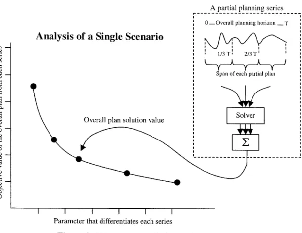
A partial planning series 0-Overall planning horizon .T

Analysis of a Single Scenario

1/3 T 2/3 T'

03 Span of each partial plan

ISolver

Overall plan solution value

0

Parameter that differentiates each series

Figure 2: The Anatomy of a Scenario Analysis

Each point on the graph is produced in similar fashion, by using a different parameter value and solving a partial planning series. The scenario under analysis determines such values as the demand function (shown here under the partial planning horizon) and other network parameters (not shown) contained in the partial plans.

single plan is called the overall plan. The length of a partial plan is the number of time periods over which it plans; the span is the set of time periods a partial plan contributes to an overall plan. A (partial planning) series is a collection of consecutive partial plans that

together make up an overall plan. Data used to analyze each scenario in Chapter 5 is gathered by generating and solving a number of partial planning series, for the same overall planning horizon, that differ only by one or two parameters. For each of the two scenarios in Section 5.1, the parameter that varies from series to series is partial plan length. The scenario in Section 5.5 contains series differentiated both by partial plan

(24)

length and replan delay time. The analysis then consists of plotting the gathered data and

interpreting the graph. Figure 2 illustrates the relationships between these terms.

The network flow problem contained in each scenario has a specific set of

network conditions. A network's conditions are its parameters (like demand) and

characteristics (deterministic vs. stochastic demand, periodic vs. on-demand replanning,

etc.) We use the term stochastic network conditions to refer to a network with one or

more parameters or characteristics that behave unpredictably over time. Stochastic

demand indicates that the demand function over a time horizon can deviate randomly

from the values used to plan for that horizon.

An overall solution is the cost of executing all partial plans in a series (in effect,

executing the overall plan for an overall planning horizon). This cost is the sum of the

execution costs expressed by each partial plan's objective function value. An efficient or

cost-effective solution is an overall plan for an overall planning horizon whose total

objective value (execution cost) is lower than that of other overall plans in the same

scenario analysis. An optimal solution is more efficient than any other solution to the

same scenario.

3.2 Formulating the Model

A problem formulated as a linear program and formatted for use with a

(25)

structure of the network (nodes and edges), the equation for the objective function, any

named sets (i.e. the set of airplanes or the set of supply warehouses), all parameters and

decision variables, and the equations (in terms of parameters and decision variables) for

constraints present in the network. In essence, the model represents an entire class of

possible problem instances. The data refers to all information that is specific to a single

instance of the problem defined in the model. It includes the members of defined sets

(i.e. the name of each warehouse) and the values for defined parameters. The demand

function and any equation coefficients are also declared as part of the data. The

Appendix contains sample model and data files to illustrate the distinction.

3.3 Finding a Solution

Solving an instance of a problem requires feeding the model and the data to a

computer program designed to solve generic linear and mixed integer programming

problems. All problems presented in this thesis were solved using a commercial software

package, CPLEX 6.6.0 with AMPL. AMPL facilitates the formulation of the model and

data with its own programming language. The model and data are first defined in

separate files, each with its own syntax. Then the two files are entered into the AMPL

command processor. The processor combines the model and the data into a complete

problem, formats the problem for solution, and sends the formatted problem to CPLEX.

CPLEX does the work of finding an optimal solution, and then passes the results back to

AMPL for display. The model and data files in the Appendix are written in AMPL's programming language.

(26)

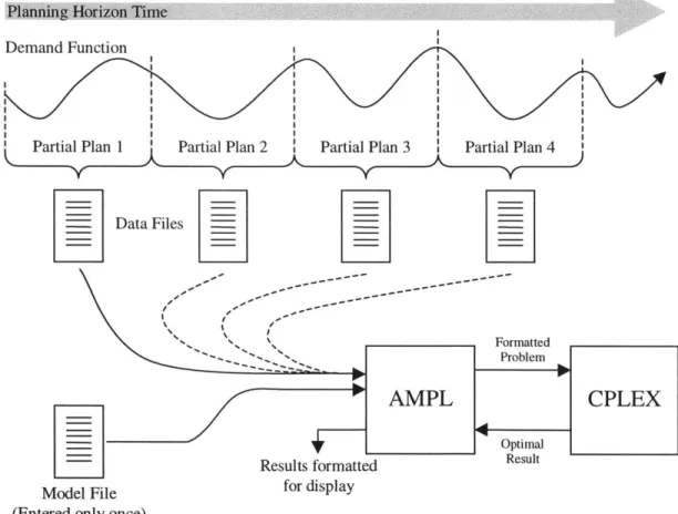
3.4 Solving a Partial Planning Series

Plugging a model and a data file into AMPL and finding a solution constitutes the

generation of a single partial plan. Since the model defines the structure of the problem

and not its specific instance, it remains largely unchanged for each partial plan of a single

partial planning series, except for minor modifications to the objective function.

Successive partial plans cover different spans of time from the problem's planning

horizon, so each plan requires its own data file. Thus a partial planning series for a long

overall planning horizon is typically made up of a single model file and a series of data

Planning Horizon Time Demand Function

Partial Plan 1 Partial Plan 2 Partial Plan 3 Partial Plan 4

Data Files

Formatted Problem

AMPL CPLEX

-- 1 Optia

Results formatted Result

Model File for display

(Entered only once)

Figure 3: Solving a Partial Planning Series

Each data file contains a section of the demand function, as well as any other network parameters. The model file is first entered into AMPL. Then a single data file is entered. AMPL then sends the complete formulation to CPLEX, which solves the problem and returns the result

(27)

files that contain separate sections of the network's parameter values (over time). To

solve a partial planning series, the model file is first entered into AMPL, and then each

data file is entered and solved in turn. See Figure 3 for a detailed illustration of this

process.

Each successive partial plan builds on the partial plans developed so far. The

partial plan for time periods 100-120, for example, is not solved in a vacuum; the plans

developed for periods 0-100 provide the initial network conditions (including flow) for

the 100-120 partial plan. These initial conditions are implemented by first loading the

solution to the previous partial plan into AMPL along with the new partial plan's data

file, and then fixing those loaded values. New partial plans take as fixed the decisions

made by all prior partial plans in a series, because in a real execution those decisions

would already have been carried out by the time the new partial plan takes effect. When

decision variable values are fixed, the solver treats them as network parameters.

Once the initial conditions are fixed, the objective function is changed to calculate

cost only for the span of time periods covered by the new partial plan. At the end of the

series, when all partial plans have been solved, the overall objective value of the solution

to the series is the sum of each partial plan's objective function value. This value

(28)

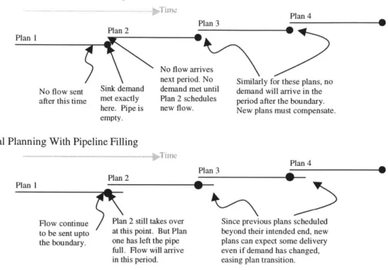
3.5 Flow Pipelining

The overall plan produced by solving a partial planning series is used to schedule

flow through the network for the duration of the overall planning horizon. Regardless of

the length of each partial plan, their combination must manifest itself as a continuous

flow schedule over time. Even though an overall plan for 200 periods may have been

generated by a series of 20-period partial plans, the execution of that overall plan over

those 200 periods should seem as if the whole horizon were planned at once. If each

partial plan considered the end of its 20 periods as the end of the entire overall plan, flow

would stop temporarily at each boundary between consecutive partial plans. The partial

plans would have no reason to send any flow that would arrive after the ends of their own

spans.

In order to avoid stopping flow between spans of partial plans in a series, the flow

schedule must be viewed as a pipeline of flow from source to sink. The flow pipeline for

the case study network is made up of discrete trucks and trains. Each truck or train takes

a certain amount of time to travel from depot to port. Without flow pipelining, each

single partial plan sends only the necessary flow to fulfill demand for its span of time. If, for example, a train takes four periods to reach its destination, no train would ever

intentionally be sent later than four periods before the end of a planning span.

Nevertheless, efficient flow across partial plan boundaries demands that the pipeline be

kept as full as possible. To this end, in every scenario in Chapter 5, each partial plan

(29)

Partial Planning Without Filled Pipeline Plan 4 Plan 3 Plan 2 Plan I No flow arrives

next period. No Similarly for these plans, no No flow sent Sink demand demand met until demand will arrive in the after this time met exactly Plan 2 schedules period after the boundary.

here. Pipe is new flow. New plans must compensate. empty.

Partial Planning With Pipeline Filling

Plan 4 Plan 3

Plan 2 Plan 10

Flow continue Plan 2 still takes over Since previous plans scheduled to be sent upto at this point. But Plan beyond their intended end, new the boundary. one has left the pipe plans can expect some delivery

full. Flow will arrive even if demand has changed, in this period. easing plan transition.

Figure 4: Flow Pipelining across Partial Plan boundaries

Each Plan (shown as a horizontal line representing the time over which it plans) is a partial plan in a series with the other plans adjacent to it. The dots represent the ends of each partial plan's span. Note that with pipeline filling, partial plans actually extend beyond their spans.

plan takes over, the pipeline is not empty. See Figure 4 for an illustration of this

(30)

4. The Case Study Model

The test problem for analyses in this thesis involves military logistics planning

and execution. The United States military has conventional ammunition storage depots

spread throughout the interior of the country. During peacetime these depots act

primarily as long-term storage. But during armed conflicts, these depots supply the bulk

of US forces overseas with conventional munitions. Over the duration of the conflict, the

bulk of the munitions from these depots must be transported to ports on the proper coast,

and then taken by ship to the overseas theater of war. In a worst-case scenario, the

United States would have to sustain two full-scale armed conflicts, one in Asia (off the

West Coast) and one in the Near East (off the East Coast). Such a scenario would require

the use and supply of all interior depots and coastal ports, with sustained heavy demand.

This is the scenario assumed for analysis.

This chapter describes a network flow problem and a linear program formulated

to model the existing conditions of the military supply infrastructure. Munitions are

stored at five primary depots, which serve as the source nodes in the flow-based network.

There are three coastal ports, two on the West Coast and one on the East Coast. Because

we are modeling conflicts across both oceans, all three ports will be utilized. For the

purposes of this thesis, only the supply network from depot to port is considered.

Demand at each port is modeled as the recurring arrival of discrete ships, but the shipping

(31)

4.1 Transportation

Between the depots and the ports is a ground transportation network. This

network involves two means of conveyance: truck and rail. Trucks typically have shorter

transport times than rail, but carry less capacity and are more expensive to operate. In

general, rail is the preferred mode of transport unless time constraints dictate the use of

more expedient means. For analyses involving stochastic transportation delays, rail

transport has a higher incidence of delay than truck transport [8].

4.2 Containers, Depots and Ports

The munitions themselves are modeled as the types of containers in which they

are shipped. Depots store munitions safely spread out in fortified bunkers. Before

munitions can be shipped, they must be packed into shipping containers. The model

allows twenty distinct container types. The container types represent different

configurations of munitions within a single container. Overall demand for munitions is

quantified as demand for each specific container configuration. Likewise, total supply at

each depot is composed of the supplies of each container type.

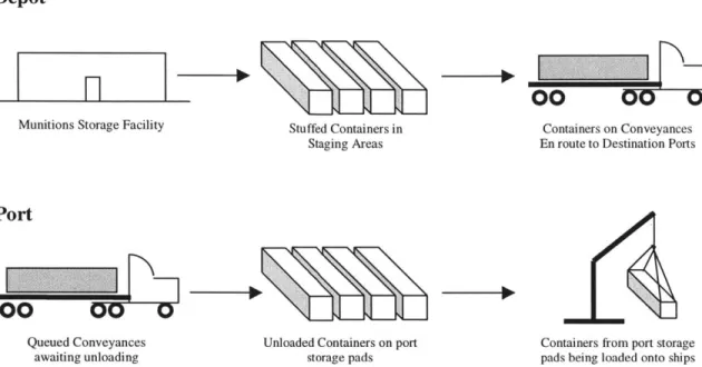
In our example problem, container stuffing at the depots takes one time period.

After being stuffed, the containers are assumed to be placed on staging areas in

preparation for shipping. Each depot has limited stuffed-container storage space, of

which each type of container requires an equal amount. Similarly at the ports of

(32)

Munitions Storage Facility _{Stuffed Containers in} Staging Areas

Queued Conveyances Unloaded Containers on port

awaiting unloading storage pads

00

-Containers on Conveyances En route to Destination Ports

400

Containers from port storage pads being loaded onto ships

Figure 5: Munitions Movement through Depot and Port

eventual movement to and loading onto ships. It is from the container stock on these

storage pads that port demand is met. In addition, each depot has a container generation

rate that specifies how many total containers the depot can stuff per time period.

Likewise each port has a specific rate at which containers can be unloaded from

conveyances. Figure 5 illustrates the stages of container movement from depot storage

facilities to ship loading areas.

4.3 Net Explosive Weight

Safety is a primary concern when munitions are being moved. Restrictions on the

total effective amount of explosive material (Net Explosive Weight, or NEW) present at

Depot

(33)

each depot and port are limited by NEW restrictions. Each container type is assigned a

NEW value based on its contents; the number of each container type at a single location

multiplied by the NEW value for each container type determines the total NEW present at

that location.

4.4 Late Delivery

Although the ideal solution to the munitions transportation problem would fulfill

all demand requirements exactly on time, this goal is not always attainable. The model

allows for late arrival of demand, but assesses a heavy penalty for every period a

container arrives past its intended arrival time. Clearly late arrivals are discouraged, but

sometimes necessary if demand increases unexpectedly during plan execution or if the

system does not have sufficient throughput capability to meet demand. Late flow is

modeled by network edges that progress backwards through time, one period at a time, at

port storage pads. Thus a container that arrives at time 3, but was intended to arrive at

time 1, would flow on late arcs from time 3 to time 2, and then from time 2 to time 1. In

traversing two late arcs, the container would thus be penalized for arriving two periods

late.

4.5 Decision Variables

The decisions to be made in the course of generating a feasible plan to solve this

(34)

Time

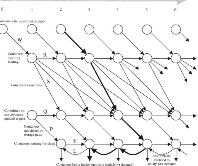
0 1 2 3 4 5 6

Containers being stuffed at depot

W0\ Containers _R awaiting _{_0} loading X Conveyances in transit Containers on

Q

conveyances queued at port Containers transferred to P storage pads Containers waiting for ships

L

Late arrivals intended to Containers being loaded onto ship (satisfying demand) satisfy past demand

Figure 6: Container Movement Network, from Depot to Port over Time Each edge represents a decision variable in the model. Each row of nodes is a single physical location. Each column is the flow to and from every location in a single time period. Arcs that travel vertically carry flow from one location to another. Horizontal arcs represent flow that remains in the same location for more than one time period. The bold edges illustrate the flow of a container stuffed at time 2 and intended for delivery at time 3. Although containers don't actually travel back in time, they flow to earlier time periods to fill unsatisfied past demand and indicate the number of late containers per period.

munitions from depot storage facilities to port shipyards in a time-space network [1].

Each node in the figure represents a physical storage location at a depot or port, and each

edge represents the movement of munitions. The quantity of ammunition associated with

(35)

right; each horizontal row of nodes is actually the same location at a different time. The

edge labels correspond to the decision variables as described in the model formulation

(Section 4.7), and text labels are also provided. For the sake of simplicity, Figure 6 only

depicts a single depot and port, and edges for the flow of one container type. The

complete problem network has similar connections to the one shown, but many more

nodes and edges.

4.6 Objective Function

The best solution to this problem delivers all required demand in the most

cost-effective manner possible. Several factors contribute to the total cost of munitions

shipped during a plan's execution. Each truck or train costs some amount per container

to operate. A severe penalty for late containers is applied in order to ensure timely

delivery whenever possible. Transporting any amount of explosives is a dangerous

undertaking, and transporting more at once increases the chances of an accident

occurring; therefore a penalty for the total NEW in transit per time period is assessed to

limit the total amount being transported at any one time. Finally, there is an added cost

for queued conveyances at ports; while they are waiting to be unloaded, they are not

being used for further transit. The exact function, in terms of decision variables and

(36)

4.7 Mathematical Formulation

The mathematical formulation for the test problem, taken from [4], is given

below. The linear program used to generate the results found in this thesis is based

directly on this formulation.

SETS

* Ns - The set of depots

* Nd - The set of ports

" V - The set of conveyance types

" B - The set of container types

DECISION VARIABLES

* Xbijkt - the flow of container type b e B from depot i E Ns to port

j

e Nd on

conveyance k e V at time t = 0, 1, 2, ...

" Q jkt - the number of containers of type b e B on conveyances of type k e V

enqueued at port j E Nd at time t = 0, 1, 2,...

" Ybjkt - _{the number of containers of type b e B at port}

j

_E_{Nd that are unloaded}

from conveyances of type k e V at time t = 0, 1, 2, ... and taken to port storage pads

* Pbjt - the number of containers of type b e B at port

j

e Nd that are located on

port storage pads and ready for retrieval for ship loading at time t = 0, 1,

2, ...

" Rbit - _{the number of containers of type b e B already stuffed and waiting in} staging area for transportation at depot i e Ns at time t = 0, 1, 2, ...

" Wbit - _{the number of containers of type b e B stuffed and delivered to staging} pads for transportation at depot i e Ns at time t = 0, 1, 2, ...

* Ljb(t+1)t - _{The number of late containers of type b e B which arrive one period late}

(37)

PARAMETERS

" Tijk - travel time from depot i e Ns to port

j

e Nd on conveyance k e V

" s b - supply of container type b _e _{B at depot i}_e _{Ns over the entire planning} horizon

" d"jt - _{demand of container type b e B at port j e Nd at time t = 0, 1, 2,}

" c ijk - unit cost of moving container type b e B from depot i e Ns to port

j

e Nd on conveyance k e V

" gjk - maximum number of containers unloaded from conveyance k _e _{V at port}

j

e Nd per time period

* nb - Net Explosive Weight of container type b e B

Sli

- maximum accumulation of NEW allowed on storage pads at port

j

e Nd * fjk - detention costs per container per time period on conveyance k e V

queued at port

j

e Nd

* - the maximum container stuffing rate for depot i e Ns

STli

- maximum accumulation of NEW allowed in staging areas at depot i e Ns g - unit safety penalty cost of NEW in the transportation network

l

lcjb - the per-period cost of late arrival of container type b E B to port

j

e Nd

* prijb - the relative priority of on-time delivery of container type b e B to port

j

E Nd

OBJECTIVE FUNCTION

Minimize:

cX + f Q +g n R + Q ,+p

t=O be B (ij,k) je Nd keV beB beB iE Ns je Nd kEV

T

+~ I I I1c jb pri _jb(t+L)t t=O jENd beB

(38)

CONSTRAINTS Subject to: T t=b W b+R _ -R, b Vi e Ns,be B -XXt =0 j,k Vie Ns,be B,t=0,...,T X b +Q (t1-Q Yb =0 ieNs Jyb _Y +pb_+Pa jk(t-1) j(t-1) keV pb _it d b_jt beB beB n R bEB bE=B

All Flows Al Fow W Wt Rb it' Xh ijkt'jQkt'I jkt' Qb Y pb jtIb(t+1)_L >0 and integer.

Vje Nd,k eV,be B,t =0,...,T Vj e Nd,be B,t =0,...,T Vie Ns,t=0,...,T Vje Nd,k eV,be B,t =0,...,T Vie Ns,t=0,...,T Vj e Nd,t =0,...,T

(39)

5. Analyses and Results

For an explanation of the terms used throughout this chapter, refer to Chapter 2 and

Section 3.1.

In this chapter we present a number of scenarios that model situations

encountered during the planning and execution of real-time network flows. Each

scenario is planned using specific variants of the partial planning approach. These

variants of the approach include altering the length of each partial plan, generating new

partial plans on either a periodic or on-demand replanning schedule, and changing the

allotted replan delay time for partial plan integration. Each analysis is designed to

provide insight into the effectiveness of the partial planning approach as it could be

applied to a real-would scenario. The analysis of each scenario consists of solving a

number of partial planning series (as described in Section 3.4), each of which uses a

different variant of the partial planning approach, and determining which variant

produces the most cost-effective solution to the network flow problem in that scenario.

5.1 Partial Plan Length

The munitions logistics planning problem involves the transportation of munitions

from interior depots to coastal ports to satisfy the demand for munitions overseas. This

(40)

duration of involvement. The duration of the conflict, and consequently the duration of

demand, is not known but assumed to be extensive. A transportation schedule needs to be

devised to move ammunition efficiently from depots to ports through a ground

transportation network for the duration of the conflict. Once devised, the schedule must

be executed and munitions shipped according to it. Since the extent of the planning

horizon for this problem cannot be determined, a sensible approach is to solve and

execute successive partial plans, each spanning a finite length of time, until supply is no

longer demanded.

5.1.1 Partial Plan Length Scenario Description

At the start of the conflict, the transportation network is assumed to be empty - all

conventional munitions are in depot storage facilities. Once the demand for munitions

begins, a partial plan is solved for some number of periods, and depots start to send

supply to ports following that partial plan. When the partial plan ends, a new partial plan

is solved and executed. In real-world execution this process would continue indefinitely,

or until demand ceases. In this scenario, indefinite demand is approximated using an

overall planning horizon significantly longer than the length of a single partial plan. The

analysis is concerned with optimizing the solution to a long overall planning horizon

using a periodic replanning approach. For the purposes of this analysis, replans only

occur periodically, and each partial plan in the same overall plan has the same length.

We are also interested in discovering how overall solutions generated using the periodic

(41)

We present two separate scenarios for comparison. The first contains a strictly

deterministic demand function that changes predictably over time, and no stochastic

network events. The second incorporates stochastic demand changes and transportation

delays. In both scenarios, once a partial plan begins execution, it cannot be changed - the

plan must be followed exactly. To analyze each scenario, we define a single demand

function over a 400 period horizon. We then use the process described in Section 3.4 to

solve a number of partial planning series. Each series is solved using a different length

for the partial plans. When the objective function values for each series' solution is

plotted against the partial plan length for that series, the relationship between partial plan

length and overall objective value for the particular network conditions of the scenario

will be known. These relationships satisfy the first objective of this thesis (see Section

2.2).

In the stochastic demand scenario, several types of events could occur over the

course of a single partial plan's execution. First, demand for munitions could change

unexpectedly. Second, the truck and rail transportation plans produced by each partial

plan may not be met during execution. In the model transportation delays occur with

small probability each time a vehicle is sent from a depot to a port. For rail, the values

used are: 5% chance of single-period late arrival, 2% chance of three-period late arrival,

and 1% chance of five-period late arrival. All trucks have a 4% chance of being delayed

one period. These numbers are not derived from actual data, but are intended to produce

sufficient delay to affect solution quality without rendering all partial planning series

(42)

In both scenarios the demand profiles (at the port of embarkation) are derived

from a schedule of ship arrivals and departures. Each port has a schedule of ships that

arrive to be loaded, depart for abroad to be unloaded, and return to be loaded again. In

the stochastic demand scenario, increases in munitions requirements overseas cause the

temporary addition of extra cargo ships to each port at various times during the scenario's

execution.

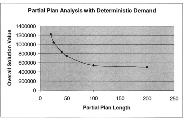
5.1.2 Deterministic Demand Results

Figure 7 shows the relationship between partial plan length and overall objective

value in the deterministic demand scenario. In the absence of stochastic events, the

Partial Plan Analysis with Deterministic Demand 1400000 4) 1200000 C 1000000 0 800000 600000 i 400000 R nw 200000 0 0 50 100 150 200 250

Partial Plan Length

Figure 7: Periodic Partial Planning with Deterministic Demand (Lower overall solution value is better)

(43)

model can accurately predict and schedule on-time delivery of all demanded munitions.

Long partial plans achieve greater solution efficiency and drive down the objective cost

of plan execution because they each have more information with which to make optimal

decisions.

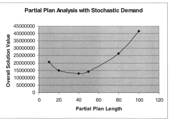
5.1.3 Stochastic Demand Results

Figure 8 relates partial plan length to objective value when the transportation

network and demand function are subject to stochastic events. The results show that the

events have a negative impact on both small and large partial plan lengths. Very small

partial plans suffer because they may need to send large amounts of ammunition to

Partial Plan Analysis with Stochastic Demand

45000000 40000000 35000000 30000000 25000000 0> 20000000 -15000000 0 U U U . ...--- *... ... . 0 f I f Af . ..---6... i10000000 - -0 5000000 - -0 0 20 40 60 80 100 120

Partial Plan Length

Figure 8: Periodic Partial Planning with Stochastic Demand Also includes random transportation delays. Lower overall solution value is better

(44)

supply excess demand from previous events, and lack the time to do so at low cost. Very

long partial plans also perform poorly because events that occur early in each partial

plan's execution are not compensated for until the beginning of the next partial plan,

causing significant late demand penalties. In-between these two extremes a better

solution can be obtained. Mid-length partial plans (about 40 periods long) are able to

recover faster than long partial plans from stochastic network events, and send flow more

efficiently over longer periods of time than short partial plans.

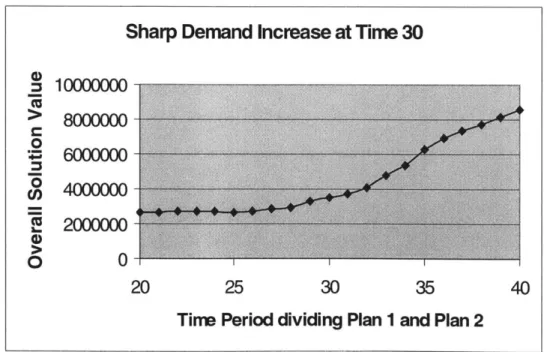
5.2 Forecasting Demand

Warfare is inherently unpredictable. Logistics support must be able to adjust to fit the needs of the battlefield. Without knowing the future, logisticians can only act based

on prediction and intelligence. In a real-time system, information about what has

happened before and what might happen soon has a serious impact on the immediate

decisions that must be made. Better forecasting and information assessment leads to

overall plans that more closely match actual conditions and result in more efficient

solutions.

Our second objective is to answer the following question: what is the qualitative

value of more accurate information on past, present and future demand conditions?

Accurate information is essential to achieving optimality when applying deterministic

planning methods to scenarios in which substantial stochastic demand events can occur,