Impacts of Fed’s decisions on emerging countries : an empirical analysis & investment solution

(1)

Impacts of Fed’s Decisions on Emerging

Countries: An Empirical Analysis &

Investment Solution

Bachelor Project submitted for the degree of

Bachelor of Science HES in International Business Management

by

Simon AMIGO WEIDEMANN

Bachelor Project Advisor:

Kurt STERCHI, Lecturer

Jury:

Ali ALTINSOY, Piguet Galland

Geneva, August 23rd, 2019

Haute école de gestion de Genève (HEG-GE)

International Business Management

(2)

(3)

Declaration

This Bachelor Project is submitted as part of the final examination requirements of

the Haute école de gestion de Genève, for the Bachelor of Science HES-SO in

International Business Management.

The student accepts the terms of the confidentiality agreement if one has been

signed. The use of any conclusions or recommendations made in the Bachelor

Project, with no prejudice to their value, engages neither the responsibility of the

author, nor the adviser to the Bachelor Project, nor the jury members nor the HEG.

“I attest that I have personally authored this work without using any sources other

than those cited in the bibliography. Furthermore, I have sent the final version of

this document for analysis by the plagiarism detection software stipulated by the

school and by my adviser”.

Geneva, August 23

rd

(4)

Acknowledgments

First of all, I would like to use this opportunity to thank SingAlliance (Switzerland)

SA and SingAlliance Pte Ltd for their unlimited support and absolute trust.

Furthermore, I would like to express my gratitude to my supervisor Mr. Kurt Sterchi,

who allowed me to explore the subject without barriers nor constraints. As a result,

I could learn solidly and comprehensively from all areas of interest wanted. I would

also like to thank Mr. Ali Altinsoy, who was quickly interested in the project and

took on his precious time to follow and advise this paper.

Moreover, I am deeply grateful to the people who have allowed me to debate and

discuss the fundamentals of financial analysis in this ever-changing industry.

Mrs. Lanhua Yu, who helped me to formulate my first hypothesis. Mr. Edouard de

L'Espée, who shared all his economic knowledge and financial experience.

Without forgetting, Mr. Laurent Perusset, who with his precise and always relevant

comments allowed me to understand and correct ideas that were sometimes too

abstract or too succinct. Their experience, opinions, and insights were an

incredible source of inspiration and knowledge.

I also would like to thank Dr Aftab Kahn for his advice. Thanks to these, I was able

to come back on a subject which I am passionate about, which lead me to continue

studying and analysing this exciting area, which is Economy.

Finally, I would like to acknowledge Mr. Nicolas Montandon, who showed great

understanding and allowed me to change the subject of a previous project when I

was in a dead-end situation.

All the people and companies mentioned above have been essential for this paper,

and I would like to thank them one last time for their collaboration and investment.

(5)

Executive Summary

On July 13

th

_{, 2019, the Fed decided to reduce its interest rates by 25 basis points.}

Its first since October 2008. A decision that could be thought of as a good thing for

the emerging countries’ economies. Indeed, according to economic theories and

history, they would benefit from a significant breath of fresh air. Legend has it that

the Fed's will have a significant impact on emerging countries, whether positive or

negative.

One could, therefore, question why did Argentina’s stock exchange – just a few

weeks after the so-called beneficial decision of the US central bank – lose 48% in

one trading session. The second-largest stock market sell-off in history after Sri

Lanka’s civil war outbreak in 1989 (-61.7%). Obviously, the reasons for this

Argentine air gap have endogenous roots, mostly political, but it is then interesting

to investigate if the Fed’s decisions impact the emerging regions of the world. Do

this relation still exists today? Have emerging countries emancipated themselves

from the American game? And finally, depending on the answers, what would be

the most efficient ways to invest in these regions, rationally and professionally.

This paper, therefore, tries to demonstrate whether the impact on emerging

markets of the Fed's decisions on rates still exists. More precisely, the approach

here is to investigate the reactions of emerging currencies against the US dollar

when interest rates vary. Through a statistical analysis over two periods (1997-

2008 and 2008-2019), using tools such as linear regression and correlation

observation, and adding the time-lag component, interesting results emerge.

Indeed, depending on the period chosen, they are diametrically opposed. As things

stand, the study shows a causal relationship and a correlation between interest

rate decisions and emerging currencies. However, the change in US rates does

not explain all the variation in the analysed currencies. The economic cycle in

which the analysis was made must also be considered, it is likely that the latter is

a significant component. The addition of variables would improve the performed

statistical model, thus allowing a better understanding of their behaviour and so

facilitate the investment process.

On this basis, adjusted with informed insights and experience of professionals, but

also with the attempt to reduce cognitive biases to a minimum, this paper

concludes with an investment solution. More specifically, a quantitative stock

selection tool based on the mixed implementation of fundamental and technical

analysis, which now shows encouraging results.

(6)

Impacts of Fed’s Decisions on Emerging Countries: An Empirical Analysis

& Investment Solution ... 1

Declaration ... i

Acknowledgments ... ii

Executive Summary ...iii

Contents...iv

List of Tables ...vi

List of Figures ...vi

Abbreviations and acronyms ...vii

1. Introduction ... 1

1.1 Literature review ... 1

1.2 US Federal Reserve ... 2

1.2.1 Fed’s history ... 2

1.2.2 Fed’s structure & functioning ... 3

1.2.3 Fed’s roles ... 4

1.2.4 Fed’s toolbox ... 5

1.2.5 Fed’s independence ... 7

1.3 Emerging markets ... 8

1.3.1 Definition ... 8

1.3.2 Investing in emerging markets ... 9

1.4 Current economic context ...10

1.5 Latest comments ...11

2. Analysis ...14

2.1 Hypothesis ...14

2.2 Methodology ...14

2.2.1 Objective ...14

2.2.2 Linear regression ...15

2.2.3 Economic time lags ...16

2.3 Results...18

2.3.1 Comments ...24

3. Discussion ...25

(7)

3.1.1 Interviews ... 25

3.1.2 Interviewees biographies ... 25

3.1.3 Interviews summary ... 28

3.2 Investment tool ... 30

3.2.1 Financial analysis ... 30

3.2.2 Methodology ... 35

3.2.3 Application ... 38

3.2.4 Performance ... 40

3.2.5 Comments ... 41

4. Conclusion ... 42

5. Bibliography ... 46

Appendix 1: Observed data ... 48

Appendix 2: STATA code (.dofile) ... 53

(8)

List of Tables

Table 1 – Regression summary 1997-2007 period ... 19

Table 2 – Regression summary 2008-2019 ... 20

Table 3 – Regression summary 1997-2007 with current account variable ... 21

Table 4 – Regression summary 2008-2019 with current account variable ... 22

Table 5 – Comparison avg. Current Acc. (% GDP) and avg. Coefficient ... 23

Table 6 - Correlation between Fed rate and EM Currency ... 23

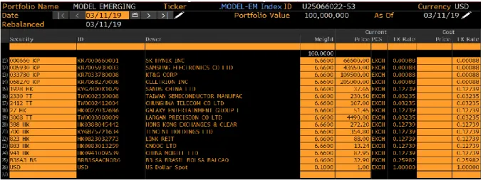
Table 7 – Virtual portfolio EM – Holdings (March 11th, 2019) ... 38

Table 8 – Risk Scenarios – Bloomberg ... 41

List of Figures

Figure 1 – Economic cycles ... 6

Figure 2 – Emerging & Frontier markets repartition ... 9

Figure 3 – Virtual portfolio EM – Currency Allocation (March 11th, 2019) .... 39

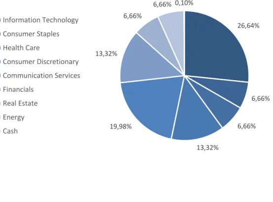
Figure 4 – Virtual portfolio EM – Sector Allocation (March 11th, 2019) ... 39

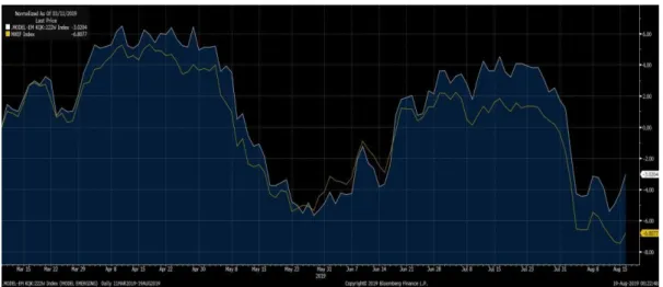
Figure 5 – Virtual portfolio EM – Performance vs. MSCI EM ... 40

Figure 6 – Virtual portfolio EUR – Performance vs. EurxStoxx50 ... 42

Figure 7 – Virtual portfolio CHF – Performance vs. SMI ... 43

(9)

Abbreviations and acronyms

(in alphabetical order)

CEPII

Centre d'Etudes Prospectives et d'Informations Internationales

GDP

Gross Domestic Product

IMF

The International Monetary Fund

MTD

Month-to-Date

OECD

Organisation for Economic Co-operation and Development

PE ratio

Price-to-Earnings ratio

RSI

Relative Strength Index

S&P 1200

Standard & Poor’s 1200

S&P 500

Standard & Poor’s 500

WACC

Weighted Average Cost of Capital

YTM

Year-to-date

(10)

(11)

1. Introduction

Does the Fed’s decisions impact emerging markets currencies? The current

empirical literature seems to show that, indeed, when the Fed decides to move

rates, it comes with an emerging market’s reaction.

This first section will provide an overview on emerging markets reacting to Fed’s

decisions. Then, for a global understanding, it will present the Fed’s background

with some of its essential aspects, define what emerging markets are and finally

contextualize current economic situation.

1.1 Literature review

In order not to deprive oneself of a voluminous and quality literature, it is necessary

to understand that a significant in- or outflow of capital result a reaction of the value

of a country’s currency. So basically, the focus of this paper is on, if or if not,

emerging currencies react to the Fed’s rate, or, by extension, on if a variation in

the US rate changes the geographical allocation of capital.

Some studies support the view that US rates have a role to play in the

behaviour of emerging markets. For example, Fernandez-Arias (1996) states that

low interest rates can, for a short period of time, improve a country's

creditworthiness by lowering its borrowing rates, thereby creating an increase in

demand for foreign capital. In another context, Taylor & Sarno (1997) write that the

most affected asset class remains the emerging bonds, in the sense that Fed

decisions are a significant factor in short-term investment flows to emerging

economies.

In a more behavioural aspect, Koepke (2015) shows that capital flows to

emerging markets are impacted by changes in market expectations. The study

provides strong evidence that the unexpected is a key factor in an investor's

decision to invest or withdraw and that the application of the decision itself

– to

raise or lower rates

– does not cause a change in capital flows to emerging

markets. This raises the question of how the Fed, by virtue of its primary role as

an economic stabilizer, should communicate to minimize the consequences on

capital flows to emerging countries and therefore by extension on their currencies

as well.

(12)

Conversely, some studies have failed to provide evidence that capital flows

from emerging markets are affected by US rates, but the conclusion allowed to drift

to new suggestions

– Hernandez, Mellado & Valdes (2001). They argue that the

impact on emerging markets is only felt over a very short period after the decision.

This observation reinforces the importance of the unexpected component,

especially since evidence is brought that the reaction of emerging economies is

weak in the long term, because market anticipation cancels out the surprise effect.

So, this paper will investigate how the emerging currencies react to a Fed’s

decision over time, by implementing 0-, 3-, 6-, 9- and 12-months time-lags.

The next section looks at the Fed's historical foundations, its role in the global

economy and the fears that accompany this powerful institution.

1.2 US Federal Reserve

1.2.1 Fed’s history

The Federal Reserve System or often shortened Fed is the central bank of the

United States. In 1791, the US government created the First Bank of the United

States. For twenty-five years was this bank then responsible for the issuance of

money and the regulation of credit. In 1816, after the war against the United

Kingdom from 1812 to 1815, the bank was replaced by the Second Bank of the

US, which was supposed to put an end to the galloping inflation that hit the country

after the war. In 1830, President Andrew Jackson, who wanted to rebuild the

banking and the monetary systems, dissolved the Second Bank. Since then, for

several decades, the United States has had to contend with a complex monetary

system that was based on barter between many regional currencies, known as

"green papers." This decentralized situation made any regulation impossible,

provoking numerous bankruptcies and crises.

In 1907,

happened one of the biggest banking crises in the US’s financial

history. This led to the foundation of the National Monetary Commission, which

was asked to define and implement a banking and monetary reform. This

commission responded to the Congress and was led at that time by Republican

Senator Nelson Aldrich. The report from this commission laid the foundation for the

Federal Reserve Act that was passed by Congress on December 23, 1913 and

promulgated by President Woodrow Wilson the same day. Then, the Congress set

three monetary policy goals in the Owen-Glass Act: full employment, price stability,

(13)

and moderate long-term interest rates. It is often referred to the first two factors

grouped under the term "dual purpose" or "dual mandate" of the Fed. Until today,

in addition with preventing financial and banking crises, these objectives still are

the sole purpose of the Fed.

1.2.2 Fed’s structure & functioning

The institution publishes numerous reports, such as the beige book, a summary of

the economic conditions in each state and in each region of the United States. The

Federal Reserve consists of a board of governors, the Federal Open Market

Committee (FOMC), twelve regional banks (Federal Reserve Banks), several

banks, and some advisory boards. The FOMC Committee is responsible for the

Fed's monetary policy. Today, this committee is made up of the seven members

of the board of governors and the twelve presidents of regional banks, where only

five have the right to vote at any given time.

Even though the Fed is a Federal institution, its structure is quite complicated

and tries to meet both the public’s interest and the banks. In the United States, all

commercial banks licensed to operate in more than one state are required to be

claim membership to the Federal Reserve in the region where their headquarters

are located. These commercial banks own shares of their regional central bank,

which allows to participate in the election of the Federal Reserve’s board members.

In all cases, the Fed's authority is defined by the US Congress and the latter

can exercise its congressional oversight right over the System. However, the

members of the Board of Governors, including the President and Vice-President of

the Fed, are appointed by the US President and confirmed by the Senate. It is also

the government that appoints the bank's senior officials, sets their salaries,

bonuses and other compensations. It is the federal government that receives the

Fed's profits, except for a 6% dividend that is paid to the banks member of the

system.

The federal government places the new institution under its authority by

appointing the Secretary of the Treasury (Minister of Finance) and the Controller

of the Currency as members, ending, the era of regional finance. Indeed, the

purpose of the new organization is to promote currency management and the

economy throughout the country, to allow the discounting of commercial paper and

to monitor the operation of US banks.

(14)

This system proved its worth during the 1929 crash: the solution envisaged by the

New York Federal Reserve, a monetary stimulus, would have made it possible to

emerge from the crisis. However, a serious reorganization was required and in

1935, the Federal Reserve Board became the Governor's Board. The new body

acquires control over the regional banks through the Banking Act. The Federal

Open Market Committee (FOMC) was also created. This committee is responsible

for overseeing national monetary policy and for regulating and controlling interest

rates.

In theory, these measures ensure that the Fed stays independent for

monetary policy. In practice, the Fed is continuously under pressure. And its

independence is often disputed. In 1978, the Humphrey-Hawkins Full Employment

Act redefined the Fed's mandate in terms of its even broader autonomy.

Today, the Federal Reserve or the US central bank is financially

independent. It receives no budget from either the government or the US

Congress. The Fed finances itself through the interest of public loans; commissions

on bank deposit benefits and interest on foreign exchange. This is how the Fed

manages to pay hundreds of millions of dollars to its shareholders and more billions

of dollars of surplus to the US Treasury.

1.2.3 Fed’s roles

The role of the Federal Reserve has evolved since then, and today this institution

generally acts as an independent or independent institution that does not depend

on other levels of government (as in many other countries). Like all central banks,

the Fed is responsible for developing, implementing, and controlling the state's

monetary policy. Also, the Fed has the important responsibility for maintaining full

employment conditions (generally considered to be around 4 to 5 %

unemployment) while keeping inflation at an acceptable level (usually below 2%).

It is also responsible for maintaining the stability of the country's financial system,

overseeing and regulating the banking system, providing financial services to d

posit-taking institutions, the Federal government, and foreign financial institutions.

A peculiarity of the US monetary system is that it is not the central bank (Fed) but

the Federal Treasury Department that creates the currency, unlike most other

countries.

Although, all these roles may sound simple in theory, it shows to be a delicate

balancing act when it comes to practice. Indeed, to achieve its monetary policy

(15)

objectives, the Federal Reserve has in its possession four tools, it can use at its

discretion (see figure 1).

1.2.4 Fed’s toolbox

The Fed uses four tools to reach its monetary policy objectives: reserve

requirements, the discount rate, interest on reserves and open market operations.

The most used and recent tool was given to the Fed after the 2008 financial

crisis. Interest on reserves is what is paid to banks when there is an excess of

reserves. Banks are required, by the Fed, to hold a certain percentage of their

deposits, so when this percentage is higher than that required by the Fed, the banks

receive interest on the surplus. So, depending on the rate decided by the Fed on

reserves, banks have more or less incentive to keep or lend their reserves. Thus,

by managing this rate, the Fed can increase or reduce the circulation of money.

Totally linked to the previous tool, reserve requirements set the deposit limit

that banks must keep. Thus, a decrease in the limit on the Fed's part would mean

the implementation of an expansionary policy. The opposite would logically explain

why the Fed wants to introduce a more restrictive policy.

The discount rate is the interest rate at which Reserve Banks lends to commercial

banks. Once again, by deciding at what rate the Fed wants commercial banks to

borrow from it in the short term, it decides its monetary policy: a low rate will tend

to see loan demand increase, demonstrating that the Fed’s choice to expand its

monetary policy. A higher rate would mean the opposite.

Finally, the open market operations tool is very simply used to buy or sell

government financial instruments, always according to the same monetary policy

management model.

(16)

Figure 1: Economic cycles

Growth:

-

Growth Domestic Product (GDP) growth rate raises

-

the Fed lowers interest rates, reserve requirements or acquires treasury

bonds.

-

Growing level of investments

-

Unemployment rate decreases

Inflation:

-

Abnormal GDP growth rates

-

Borrowing becomes too cheap

-

General price increase

-

Unemployment rate decreases

Slow down:

-

GDP growth rate stabilizes

-

the Fed raises interest rates, reserve requirements or sells treasury bonds.

-

Reduced investments

-

Borrowing becomes more expensive

Recession:

-

GDP growth rates decline substantially

-

Borrowing becomes too expensive

-

General price decrease

-

Unemployment rate increases

Gr ow th Inf l at ion S l_o w d_o w n Recession Gr ow th Inf l at ion

Growth: the Fed lowers interest rates, reserve requirements or acquires treasury bonds. - Growing level of investments

- GDP growth rate raises - Unemployment rate decreases

Inflation : the Fed lowers interest rates, reserve requirements or acquires treasury bonds. - Unormal GDP growth rates

- Borrowing becomes too cheap - Unemployment rate decreases - General price increase

(17)

1.2.5 Fed’s independence

Due to is role, the Fed is supposed to be independent and should act, above all,

for the better of the US economy. However, for some time now and more recently

Fed’s independence is disputed.

For example, some authors have, in the past, questioned its independence.

Indeed, some developed the thesis that the Fed would, in fact, be controlled by the

leading American private banks that could effectively defend their own interests to

the detriment of the general interest. The Fed has also recently been questioned

in several cases in which it is suspected of having been unresponsive to

questionable practices by certain major banks. It did not launch an investigation

against Goldman Sachs even though the information had been sent to it on a

contentious operation carried out at the beginning of 2012. The Fed would not have

acted on a recommendation from its 2009 team to conduct an in-depth review of

the London branch of JP Morgan bank, while it found itself in 2012 at the heart of

the financial scandal known as the "London whale."

More recently, concern about the Fed's independence has never been so

acute. Analysts, economists, and academics have been worried about this

independence, which they believe is threatened by the growing political pressure

exerted by Donald Trump. In fact, the Republican President has consistently

criticized the institution since his election. In particular, he criticizes it for

maintaining interest rates that he considers too high.

Relatively recent, the independence of the major central banks was

introduced in the aftermath of the oil shocks of the 1970s. Unelected, central

bankers are free to take unpopular measures to avoid price hikes and limit

excesses in the financial system. This freedom is essential to establish their

credibility with the markets; otherwise their measures won't work. A famous

example remains the German Bundesbank after World War II, which then obeyed

to politics, massively printed money to pay off the war debt, which triggered severe

hyperinflation for the Germans.

The following section introduces the definition of what emerging markets are and

what characterises them.

(18)

1.3 Emerging markets

1.3.1 Definition

What is emergence? Or what is an emerging country?

Simply put, emergence is a concept to describe the growing attractiveness of

developing countries with a middle-income population. With growth starting in its

own financial market, until it becomes big enough to be considered as an emerging

economy, to, finally, mature and become a developed country.

Although there is no unanimously accepted definition, the emergence concept

contains the following three elements according to the CEPII

1

definition:

-

a level of income below the OECD

2

average

-

sustained economic growth accompanied by increasing openness over a

relatively long period

-

attractiveness for international investors

Thus, this paper will define a country as emerging with the following criteria. To

understand the emergence and capacity of a country to emerge, it is necessary to

highlight the competitive capacity of its economy and being a member of the

OECD, is not enough to be categorized as a developed country.

An emerging country must be able to sustain rapid economic growth over a

significant period without jeopardizing its balance or stability. Indeed, many

candidates in the past have demonstrated legitimate growth in a short period of

time but have nevertheless found it impossible to replicate this development

capacity in the medium or long term. This has often led to a crash in the value of

the currency, periods of inflation and even hyperinflation. In the recent weeks,

Argentina has been the perfect example of this situation, a real case study.

The emergence therefore highlights the competitive capacity of the

economy. In short, it must apply the foundations of capitalist theory, which states

that when in a liberal economy, a society or, here, a country, it must know how to

allocate and use its resources as long as open and free, market and competition,

without deception nor fraud, is possible.

1

_{Centre d’Etudes Prospectives et d’Informations Internationales}

2

_{Organisation for Economic Cooperation and Development}

(19)

1.3.2 Investing in emerging markets

Investing is something one can do it anywhere in the world. The choice of

investment products that make it possible to invest in the most diverse sectors,

companies, themes, and countries of interest are vast. Emerging markets offer

particularly attractive investment opportunities. But what exactly is it about? What

are their particularities for investors?

Before making an investment in this area and including emerging market

securities in your portfolio, it is therefore recommended to get a first impression of

this sector. The easiest way to do this is to look at the "MSCI Emerging Markets"

index (see figure 2). This equity index reflects the performance of the stock markets

of 24 emerging countries. It, therefore, makes it possible to see which countries

are precisely considered emerging and how their markets are evolving.

But first, a distinction must be made between an emerging country and an

emerging economy. Korea and Taiwan are the best examples. For some

indicators, such as GDP per capita, Taiwan is considered more developed than

France or the UK. Not to mention, that both have world leaders in their field

–

Taiwan Semiconductor and Samsung - and that despite this, they still categorize

themselves as emerging markets.

(20)

For investors, these markets offer additional opportunities but also present higher

risks than industrialized countries. However, investing in emerging markets also

involves a, and often higher, risk. Political insecurity and less monetary stability

lead to increased volatility on the stock markets. As local currencies can quickly

lose value, the exchange rate risk is also higher. As it has been statistically

demonstrated, the situation in other countries also plays a role: in emerging

markets, local currencies are often highly dependent on the US monetary policy.

Similarly, the decisions taken by world powers in the context of their foreign policy

may have a greater or lesser influence on these currencies.

Moreover, in these countries, the risk of a company being nationalized cannot be

ruled out. Other additional risks include the lack of transparency in these markets.

Market regulation does not always work or is subject to slow adaptation; intellectual

property is poorly protected; these factors that can also influence the economic

and financial development of emerging markets.

1.4 Current economic context

Despite the August’s recent rollercoaster movements and the uncertainty of the

current events (US-China trade war, Iran tensions, Brexit, etc.), shares have risen

since January, and according to the experts, they should continue. So far, nothing

has seemed to derail the rise in markets since January: +15% for the S&P 500,

+16% for the SMI (data observed August 8

th,

_{2019), stock market indices have}

risen in the developed and emerging world despite several threats to the global

economy, particularly the trade war between China and the United States.

The question now would be to know if the second half will be as bullish as

the first one as growth seems to be weakening, and trade tensions are picking up

again. Credit Suisse believes so: "We believe that the upside potential is intact,

although the risks of temporary corrections after the recent rally have increased,"

says Burkhard Varnholt, Head of Investments, in a note assessing market

performance in the first half of the year and setting out the outlook for the second.

On the other hand, UBS is a little more cautious, reducing its equity allocation

from "overweight" to "neutral" for the second half of the year. Isn't this year's

rebound "too good to last"? Political risks - commercial or Brexit - could fuel

volatility, they warn, also in a 2019 mid-term study. "Investors need to be agile and

diversify their investment strategy in order to generate risk-adjusted returns," they

recommend. It is in China, above all, that they see the most opportunity on the

(21)

equity markets. Its economy is stable, investors are increasingly positive, and the

inclusion of this market in the MSCI index will make it even more critical.

Nevertheless, the bank also believes that diversification into real assets and

related alternative investments is likely to continue. For many, the rise in stock

markets should, therefore, continue, while being subject to some probable ups and

downs depending on political events. This will provide new purchasing

opportunities. Especially since the signals from the US Federal Reserve, which

seems to be considering another reduction in its interest rates, are favourable to

the markets.

Most specific to this paper’s question, Fed’s latest rate cut (25bps reduction)

could give emerging economies a breath of fresh air. Emerging economies, which

are suffering from the slowdown in world trade and, above all, the decline in

Chinese demand in goods and services, could benefit from a breath of fresh air

thanks to the Fed which recently re-opened the door to a rate cut.

1.5 Latest comments

3

Following are some interesting comments from professionals of the industry that

will be investigated in this paper.

After leaving rates unchanged a week ago, Fed boss Jerome Powell

explained on Tuesday that he did not want to "overreact" by

immediately easing the bank's monetary policy in response to fears

about trade tensions between Washington and Beijing.

Even if his speech was less accommodating than expected, he

distanced the prospect of a further rate increase, which would have

strengthened the transfer of capital to the United States, where

investments are less risky or increased the price of servicing their debt

in dollars.

"As the normalization of monetary policy in the United States is halted

or even reversed, it may ease markets and financing conditions for

emerging countries," Sébastien Jean, director of the Centre for

Prospective Studies and International Information (CEPII), told AFP.

"For some countries, there may, therefore, be some windfall effect," he

added, referring to emerging economies that can afford it. Because

3

(22)

they have the flexibility to boost their growth by financing themselves

on the markets without fear of rising interest rates.

A welcome breath of fresh air at a time when emerging economies are

experiencing growth rates driven by "low investment and the sharp

slowdown in world trade," as recently explained by World Bank

President David Malpass.

"A low rate in the United States is, a priori, good news for emerging

countries because it creates slightly stronger incentives for flows" to

these countries, Jens Arnold, head of the OECD's Department of

Economics for Argentina and Brazil, told AFP.

There is also the "risk aversion" that currently characterizes markets,

as Sean Darby, of the American investment bank Jefferies, pointed out

at a conference in Paris. "What is happening in China is necessarily

harmful to emerging countries," he told AFP about the decline in raw

material exports to the Asian giant, which have long supported

emerging economies. For Mr. Faure, the rates are too high anyway for

emerging countries to be able to finance themselves on the markets,

especially Argentina, which is in recession. "Not only do the

Argentinians not want to, but they couldn't. This is better because they

are already very heavily indebted," he said.

However, Mr. Darby noted that central banks in emerging countries are

distancing themselves from the Fed. "This time, long before the Fed

moved, several central banks in emerging countries lowered their

rates, such as Malaysia, the Philippines, and India," he said. "The

divorce between the emerging countries and the Fed has become quite

clear," said the Jefferies analyst, citing the case of Russia.

These comments could be the headlines of all the stereotypes and/or common

literature when it comes to defining emerging markets reactions to the Fed’s rate

changes. So, using statistical analysis - a linear regression - this paper will try to

unravel some of these affirmations anchored in the collective imagination.

The rest of the paper is organized as follows. Section 2. performs a statistical

model to measure Fed’s rate impact on emerging currencies. Section 2.3. shows

(23)

the results obtained by the linear regression and explains if and how emerging

currencies react to changes in US rates.

Section 3.1. explains investing in emerging markets and introduces discussions

with professionals of the financial industry about the statistical model (Section 2.)

and how investment decisions are made.

Based on financial analysis theories such as fundamental, technical and

behavioural, a quantitative investment solution for emerging markets equities is

proposed in Section 3.2. Section 4. concludes.

(24)

2. Analysis

2.1 Hypothesis

It is commonly known and said that when the Fed flaps its wings, the emerging

markets suffer an earthquake. Recently, James O’Neill, former chief economist at

Goldman and inventor of the BRIC name, said that high deficit countries would get

impacted heavily by the reduction of Fed’s quantitative easing.

The first step is the attempt to prove that emerging currencies are heavily impacted

by Fed rates. In a second step, the article wants to show that the more the current

account of a country is negative, the more the elasticity of the currency with respect

to the Fed is large.

2.2 Methodology

2.2.1 Objective

The objective of this analysis will be to analyse how the eight following emerging

countries’ currencies react to the decisions taken by the US Federal Reserve. To

achieve this, the method used will be linear regression through STATA, a

general-purpose statistical software.

The selection of currencies was based on the following reasons: First, we opted for

the selection of currencies emanating from the countries represented by the

association of the five largest emerging economies, more commonly known by the

acronym BRICS. The latter includes Brazil, Russia, India, China, and South Africa,

the latest country to join the alliance in 2010. Then, in order to identify a potential

variation originating from the geographical location, we selected additional

currencies coming from different continents, namely:

• For Africa: Nigerian Naira (NGN)

• For South America: Mexican Peso (MXN)

(25)

So, the observed pairs of currency are:

• USDTRY (Turkish Lira / US Dollar)

• USDRUB (Russian Ruble / US Dollar)

• USDCNY (Chinese Yuan / US Dollar)

• USDINR (Indian Rupee / US Dollar)

• USDBRL (Brazilian Real / US Dollar)

• USDMXN (Mexican Peso / US Dollar)

• USDNGN (Nigerian Naira / US Dollar)

• USDZAR (South African Rand / US Dollar)

Also, we will take two distinct periods into consideration in order to conduct our

analysis. The first, from 1997 to 2019, and the second, from 2008 to 2019, which

represents the start of the after-crisis US quantitative easing.

2.2.2 Linear regression

We will continue with our model that tries to explain the variation of the emerging

currencies (our dependent variable "Y") according to explanatory variables (X1).

Variable X1 corresponds to the Fed’s rate. So, our model looks like this:

where:

Y = the log (USDXXX) pair

X

1

= the Fed rate

The last term corresponds to the error term, which represents the deviation

between the models’ predictions and reality. As previously our goal here will be to

determine the significant variables, i.e., whether the different coefficients are

different from 0, the constant value of the alpha and the different "beta" coefficients

that minimize the error between our estimated linear regression line and the real

values of Y and finally the accuracy of our model, using, among other things, the

"R-squared".

(26)

Within this model, the EM currency is put to the log in order that the results are

expressed in percentage terms. In other words, to find out how much is the

percentage of changes in Y for a change in 1 unit of X.

2.2.3 Economic time lags

Those who follow the market will have noticed that economists often announce a

recession long after it has started. Indeed, time-lags or recognition lags can,

depending on the strength and nature of the economic shock, be from several days

to several months.

This economic characteristic exists because it takes time to measure the economic

activity of a country, region or larger. Data is rarely available live, and it may take

several months or quarters for some information to be collected and published. So

that they can then be analysed and correctly interpreted by decision makers. It

takes between three and six months, on average, for a lag to be seen, and it is

difficult to reduce this window, mainly due to variables presenting economic health

that are only presented monthly or quarterly.

As a result, monetary authorities are often not quick to respond to published

figures. The initial estimates reported are often incomplete and inaccurate. Indeed,

a variation in one direction or the other is often temporary and may return to normal

by the time of the next publication. This gives the government more time to analyse

trends more accurately and, if necessary, act to correct the situation. Time lags

play an essential role in the effectiveness of the economic policy. There is an

estimation of 18 months for interest rate cuts to have their full effect. This means

that the rate cuts in the US of the past few weeks, may not have their full effect

until mid-2020.

On the other hand, time lags make it very difficult for economists to try to

boost the economy. For example, if the economy is in recession, the Fed will most

likely cut its rates and the government may even lower taxes. But where it hurts is

that by the time the economy acknowledges the government's actions, the

recession will have lasted for some time, and, what is certain, the negative effects

such as rising unemployment will have already had time to be felt. The other risk

is that the government will go too hard on economic recovery and that in a year's

time it will face the onset of inflationary pressure due to the economic air call

created twelve months earlier. In other words, the main challenge for governments

is not to find out how the economy is doing but how it will do. Everything is based

(27)

on the past to establish forecasts, and every action is actually an anticipation to

control future economic conditions. They try to read the past to navigate the future

between bandwidths.

Managing time-lags could be seen as one was manoeuvring a cargo ship, where

one could only look out of the back window as economists can only see the past,

not the future. Meaning that, when you try to change sides, it takes dozens of

minutes (time Lag) for the cargo to show a response to the decision made some

time ago. Therefore, accidents could happen quickly as you are always trying to

compensate right and left to find out the correct navigation route or for

governments, the right temperature for their pressure cooker they call Economy.

Nearly every issue in economic can be subject to time-lags. An example of time

lag could be if there is a shortage of nurses. This, in theory, should push up the

wages of nurses. In the very long run, this may encourage more people to train as

a nurse. A shortage of nurses may put pressure on the government to alter its

immigration policies.

Coming back to our question and as we now understood that the economy

could be compared to a cargo ship. We decided to implement time-lags in our

analysis as well. Thus, the paper introduces time lags of 0, 3, 6, 9, and 12 months

on each regression. In doing so, we will be able to bring consistency to the analysis.

Then, to verify the second hypothesis, the current account in % of the GDP will be

added to the first regression as a new independent variable. Once with linked with

the same timeline than the Fed rate, once with the exchange rate. This will allow

us to find out if the model is improved by checking an increase in the adjusted R2.

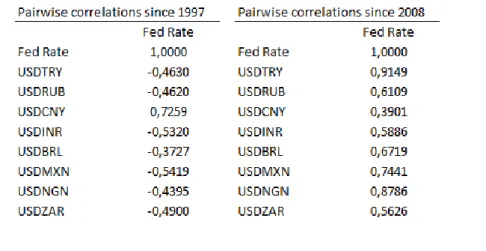
To conclude this analysis, this paper will investigate the correlation between

the rate of the Fed and the currencies in both periods. And a last linear regression

is performed on the coefficients previously with the average current accounts of

their respective periods. This will allow a thorough check to see if the current

account’s value of a country has an impact on the sensitivity of the Fed rate and

the EM currencies.

where:

Y = the log (USDXXX) pair

X

1

= the Fed rate

(28)

2.3 Results

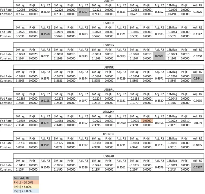
First, we can see that overall, the regression of emerging currencies relative to the

Fed rate is statistically significant for both periods (Table 1 and Table 2), despite

the simplicity of the model.

For the period 1997-2007, the first hypothesis can be refuted for all currencies. All

coefficients are negative, which means that a change in US rates would bring down

a pair of currencies, meaning a strengthening of the emerging currency. Also, there

is no consensus on the best model used. The adjusted R2s are scattered over four

of the five time-lag models.

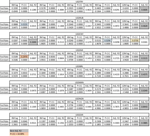
About the second period (2008-2019), there is relevancy in the numbers. Also, we

can finally see how a hike in the US rates will impact the currencies. With all

coefficients being positive, one can highlight the fact that low-interest rates result

to a capital outflow in dollars to countries with higher rates, here emerging

countries. So, when the attractiveness of the US is coming back with a rate hike,

the money will return and thus peg the countries indebted in dollars.

Another interesting observation is that the twelve-months lag is the best model for

the period except for China. China that could already be considered as an outlier

since although it is officially an emerging country, one could ask oneself, if it is

behaving like it.

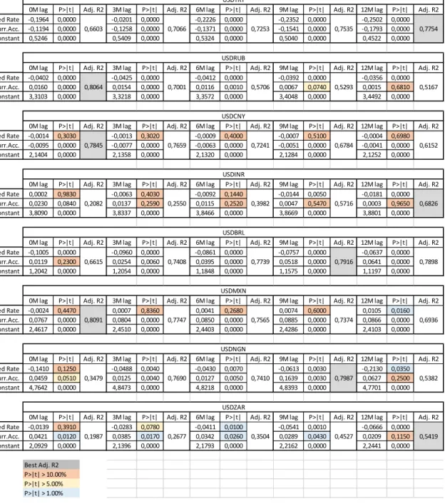
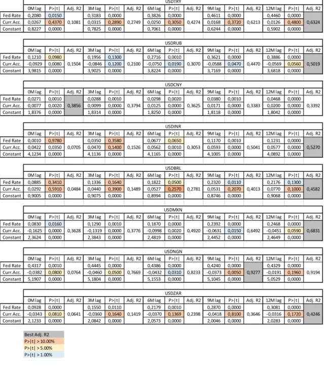
Considering the debt, when we add the variable of the current account as a

percentage of the GDP in the linear regression, we obtain a better model (Table 3

– 4). Even if some of the coefficients become statistically irrelevant, the adjusted

R2 is noticeably improved. I am proving again that the country's debt has a role to

play in the sensitivity of emerging currencies to US rates.

The models, where we linked the current account variable to the same quarter

than the exchange rate, were also better than the first ones but did not bring a better

understanding nor a better-adjusted R2.

(29)

Table 1 – Regression summary 1997-2007 period

0M lag P>|t| Adj. R2 3M lag P>|t| Adj. R2 6M lag P>|t| Adj. R2 9M lag P>|t| Adj. R2 12M lag P>|t| Adj. R2 Fed Rate -0.2098 0.0000 -0.2129 0.0000 -0.2121 0.0000 -0.2064 0.0000 -0.1976 0.0000 Constant 0.7362 0.0000 0.7333 0.0000 0.7130 0.0000 0.6723 0.0000 0.6194 0.0000

0M lag P>|t| Adj. R2 3M lag P>|t| Adj. R2 6M lag P>|t| Adj. R2 9M lag P>|t| Adj. R2 12M lag P>|t| Adj. R2 Fed Rate -0.0418 0.0000 -0.0536 0.0000 -0.0641 0.0000 -0.0735 0.0000 -0.0819 0.0000 Constant 2.1054 0.0000 2.1490 0.0000 2.1854 0.0000 2.2164 0.0000 2.2424 0.0000 Best Adj. R2 P>|t| > 10.00% P>|t| > 5.00% P>|t| > 1.00% USDZAR 0.1540 0.2526 0.3561 0.4578 0.5567 USDNGN 0.1591 0.1397 0.1231 0.1123 0.1095 USDMXN 0.1721 0.1152 0.0590 0.0156 -0.0071 USDBRL 0.6158 0.5977 0.5381 0.4530 0.3695 USDINR 0.2573 0.3344 0.4229 0.4971 0.5441 USDCNY 0.0711 0.0813 0.0873 0.0902 0.0750 USDRUB 0.1558 0.1493 0.1321 0.1183 0.1147 USDTRY 0.3670 0.3707 0.3611 0.3352 0.3026

(30)

Table 2 – Regression summary 2008-2019

0M lag P>|t| Adj. R2 3M lag P>|t| Adj. R2 6M lag P>|t| Adj. R2 9M lag P>|t| Adj. R2 12M lag P>|t| Adj. R2

Fed Rate 0.1930 0.0000 0.3178 0.0000 0.3923 0.0000 0.4403 0.0000 0.4243 0.0000

Constant 0.6949 0.0000 0.6171 0.0000 0.5704 0.0000 0.5364 0.0000 0.5251 0.0000

Fed Rate 0.0888 0.0220 0.1886 0.0000 0.2640 0.0000 0.3443 0.0000 0.3641 0.0000

Constant 3.6471 0.0000 3.5868 0.0000 3.5429 0.0000 3.5012 0.0000 3.4806 0.0000

Fed Rate 0.0287 0.0000 0.0293 0.0000 0.0240 0.0000 0.0132 0.0290 0.0110 0.0730

Constant 1.8597 0.0000 1.8605 0.0000 1.8632 0.0000 1.8678 0.0000 1.8685 0.0000

Fed Rate 0.0189 0.2970 0.0616 0.0030 0.0959 0.0000 0.1332 0.0000 0.1398 0.0000

Constant 4.0186 0.0000 3.9915 0.0000 3.9709 0.0000 3.9501 0.0000 3.9420 0.0000

Fed Rate 0.1074 0.0010 0.1840 0.0000 0.2410 0.0000 0.2890 0.0000 0.2880 0.0000

Constant 0.9193 0.0000 0.7731 0.0000 0.7398 0.0000 0.7130 0.0000 0.7021 0.0000

Fed Rate 0.0562 0.0060 0.1195 0.0000 0.1687 0.0000 0.2174 0.0000 0.2215 0.0000

Constant 2.6463 0.0000 2.6087 0.0000 2.5807 0.0000 2.5561 0.0000 2.5468 0.0000

Fed Rate 0.1698 0.0000 0.2924 0.0000 0.3736 0.0000 0.4543 0.0000 0.4472 0.0000

Constant 5.1574 0.0000 5.0859 0.0000 5.0397 0.0000 4.9981 0.0000 4.9855 0.0000

Fed Rate 0.0800 0.0040 0.1397 0.0000 0.1875 0.0000 0.2308 0.0000 0.2467 0.0000 Constant 2.2661 0.0000 2.2302 0.0000 2.2033 0.0000 2.1801 0.0000 2.1656 0.0000 Best Adj. R2 P>|t| > 10.00% P>|t| > 5.00% P>|t| > 1.00% USDTRY 0.1280 0.3084 0.4631 0.6291 0.6606 USDRUB 0.0315 0.1308 0.2457 0.3972 0.4628 USDCNY 0.2690 0.2113 0.1270 0.0298 0.0181 USDINR 0.0007 0.0604 0.1453 0.2725 0.3115 USDBRL 0.0731 0.1814 0.2970 0.4133 0.4375 USDMXN 0.0470 0.1878 0.3604 0.5725 0.6349 USDNGN 0.1369 0.3405 0.5405 0.7875 0.8443 USDZAR 0.0521 0.1356 0.2298 0.3303 0.3885

(31)

Table 3 – Regression summary 1997-2007 with current account variable

0M lag P>|t| Adj. R2 3M lag P>|t| Adj. R2 6M lag P>|t| Adj. R2 9M lag P>|t| Adj. R2 12M lag P>|t| Adj. R2 Fed Rate -0,1964 0,0000 -0,0201 0,0000 -0,2226 0,0000 -0,2352 0,0000 -0,2502 0,0000 Curr.Acc. -0,1194 0,0000 -0,1258 0,0000 -0,1371 0,0000 -0,1541 0,0000 -0,1793 0,0000

Constant 0,5246 0,0000 0,5409 0,0000 0,5324 0,0000 0,5040 0,0000 0,4522 0,0000

0M lag P>|t| Adj. R2 3M lag P>|t| Adj. R2 6M lag P>|t| Adj. R2 9M lag P>|t| Adj. R2 12M lag P>|t| Adj. R2 Fed Rate -0,0402 0,0000 -0,0425 0,0000 -0,0412 0,0000 -0,0392 0,0000 -0,0356 0,0000

Curr.Acc. 0,0160 0,0000 0,0154 0,0000 0,0116 0,0010 0,0067 0,0740 0,0015 0,6810

Constant 3,3103 0,0000 3,3218 0,0000 3,3572 0,0000 3,4048 0,0000 3,4492 0,0000

0M lag P>|t| Adj. R2 3M lag P>|t| Adj. R2 6M lag P>|t| Adj. R2 9M lag P>|t| Adj. R2 12M lag P>|t| Adj. R2 Fed Rate -0,0014 0,3030 -0,0013 0,3020 -0,0009 0,4000 -0,0007 0,5100 -0,0004 0,6980 Curr.Acc. -0,0095 0,0000 -0,0077 0,0000 -0,0063 0,0000 -0,0051 0,0000 -0,0041 0,0000

Constant 2,1404 0,0000 2,1358 0,0000 2,1320 0,0000 2,1284 0,0000 2,1252 0,0000

0M lag P>|t| Adj. R2 3M lag P>|t| Adj. R2 6M lag P>|t| Adj. R2 9M lag P>|t| Adj. R2 12M lag P>|t| Adj. R2 Fed Rate 0,0002 0,9830 -0,0063 0,4030 -0,0092 0,1440 -0,0144 0,0050 -0,0181 0,0000

Curr.Acc. 0,0230 0,0840 0,0137 0,2590 0,0115 0,2520 0,0047 0,5470 0,0003 0,9650

Constant 3,8090 0,0000 3,8337 0,0000 3,8466 0,0000 3,8669 0,0000 3,8801 0,0000

Curr.Acc. 0,0119 0,2300 0,0254 0,0060 0,0395 0,0000 0,0518 0,0000 0,0641 0,0000

Constant 1,2042 0,0000 1,2054 0,0000 1,1848 0,0000 1,1575 0,0000 1,1197 0,0000

Fed Rate -0,0024 0,4470 0,0007 0,8360 0,0041 0,2680 0,0074 0,6000 0,0105 0,0160

Curr.Acc. 0,0767 0,0000 0,0804 0,0000 0,0850 0,0000 0,0885 0,0000 0,0866 0,0000

Constant 2,4617 0,0000 2,4510 0,0000 2,4403 0,0000 2,4286 0,0000 2,4103 0,0000

Curr.Acc. 0,0459 0,0510 0,0125 0,0040 0,0127 0,0050 0,1639 0,0030 0,0627 0,2500

Constant 4,7642 0,0000 4,8473 0,0000 4,8218 0,0000 4,8393 0,0000 4,7701 0,0000

0M lag P>|t| Adj. R2 3M lag P>|t| Adj. R2 6M lag P>|t| Adj. R2 9M lag P>|t| Adj. R2 12M lag P>|t| Adj. R2 Fed Rate -0,0139 0,3910 -0,0283 0,0780 -0,0411 0,0100 -0,0541 0,0010 -0,0666 0,0000 Curr.Acc. 0,0421 0,0120 0,0385 0,0170 0,0342 0,0260 0,0289 0,0430 0,0209 0,1150 Constant 2,0929 0,0000 2,1396 0,0000 2,1793 0,0000 2,2162 0,0000 2,2441 0,0000 Best Adj. R2 P>|t| > 10.00% P>|t| > 5.00% P>|t| > 1.00% USDTRY 0,6603 0,7066 0,7253 0,7535 0,7754 USDRUB 0,8064 0,7001 0,5706 0,5293 0,5167 USDCNY 0,7845 0,7659 0,7241 0,6784 0,6152 USDINR 0,2082 0,2550 0,3982 0,5716 0,6826 USDBRL 0,6615 0,7408 0,7739 0,7916 0,7898 USDMXN 0,8091 0,7747 0,7565 0,7374 0,6936 USDNGN 0,3479 0,7690 0,7410 0,7987 0,5382 USDZAR 0,1987 0,2677 0,3504 0,4527 0,5419

(32)

Table 4 – Regression summary 2008-2019 with current account variable

Fed Rate 0,2080 0,0150 0,3183 0,0000 0,3826 0,0000 0,4611 0,0000 0,4460 0,0000

Curr.Acc. 0,0267 0,4370 0,0315 0,2890 0,0250 0,3050 0,0168 0,3720 0,0126 0,4800

Constant 0,8227 0,0000 0,7825 0,0000 0,7061 0,0000 0,6244 0,0000 0,5902 0,0000

Fed Rate 0,1210 0,0980 0,1956 0,1300 0,2716 0,0010 0,3621 0,0000 0,3886 0,0000

Curr.Acc. -0,0929 0,0080 -0,0846 0,1200 -0,0750 0,0190 -0,0588 0,0470 -0,0569 0,0560

Constant 3,9815 0,0000 3,9025 0,0000 3,8224 0,0000 3,7169 0,0000 3,6818 0,0000

Fed Rate 0,0271 0,0010 0,0288 0,0010 0,0298 0,0020 0,0380 0,0010 0,0468 0,0000

Curr.Acc. 0,0077 0,0020 0,0099 0,0000 0,0125 0,0000 0,0171 0,0000 0,0200 0,0000

Constant 1,8376 0,0000 1,8314 0,0000 1,8250 0,0000 1,8118 0,0000 1,8042 0,0000

Fed Rate 0,0010 0,9780 0,0350 0,3580 0,0677 0,0650 0,1170 0,0010 0,1231 0,0000

Curr.Acc. 0,0422 0,0350 0,0470 0,1400 0,0562 0,0010 0,0593 0,0000 0,0577 0,0000

Constant 4,1234 0,0000 4,1136 0,0000 4,1165 0,0000 4,1005 0,0000 4,0892 0,0000

Fed Rate 0,0885 0,3410 0,1336 0,1640 0,1822 0,0500 0,2320 0,0110 0,2176 0,1300

Curr.Acc. 0,0292 0,5910 0,0440 0,3900 0,0527 0,2570 0,0531 0,2070 0,0770 0,1000

Constant 0,9005 0,0000 0,9075 0,0000 0,8994 0,0000 0,8746 0,0000 0,9068 0,0000

Fed Rate 0,0830 0,0160 0,1290 0,0010 0,1870 0,0000 0,2392 0,0000 0,2468 0,0000

Curr.Acc. -0,1625 0,0000 -0,1319 0,0000 -0,0998 0,0020 -0,0631 0,0150 -0,0451 0,0590

Constant 2,3624 0,0000 2,3843 0,0000 2,4819 0,0000 2,4452 0,0000 2,4649 0,0000

Fed Rate 0,4317 0,0010 0,4445 0,0000 0,4386 0,0000 0,4240 0,0000 0,4329 0,0000

Curr.Acc. -0,0382 0,0800 -0,0460 0,0500 -0,0432 0,0310 -0,0373 0,0050 -0,0191 0,1960

Constant 5,1907 0,0000 5,1804 0,0000 5,1553 0,0000 5,1045 0,0000 5,0529 0,0000

Fed Rate 0,0928 0,0000 0,1550 0,0110 0,2179 0,0010 0,2870 0,0000 0,3081 0,0000 Curr.Acc. -0,0343 0,0810 -0,0360 0,1640 -0,0370 0,1369 -0,0418 0,8100 -0,0316 0,1720 Constant 2,1233 0,0000 2,0842 0,0000 2,0573 0,0000 2,0046 0,0000 2,0283 0,0000 Best Adj. R2 P>|t| > 10.00% P>|t| > 5.00% P>|t| > 1.00% USDTRY 0,1081 0,2749 0,4274 0,6213 0,6324 USDRUB 0,1504 0,2100 0,3070 0,4470 0,5019 USDCNY 0,3856 0,3794 0,3625 0,3383 0,3392 USDINR 0,0705 0,1526 0,3053 0,5041 0,5270 USDBRL 0,0484 0,1489 0,2781 0,4013 0,4582 USDMXN 0,3628 0,3776 0,4920 0,6492 0,6831 USDNGN 0,0764 0,7669 0,8233 0,9277 0,9194 USDZAR 0,0641 0,1419 0,2398 0,3646 0,4246

(33)

Table 5

– Comparison of Average Current Acc. (% GDP) and Average

Coefficient over the analysed periods

With Table 5, we realize that there are no rules that can be deduced with a

comparison between the current accounts and the regression coefficients. Indeed,

a change in the current account does not necessarily have an impact on the

coefficient of the regression.

However, with Table 6, it becomes evident that the economic cycle has a real

impact on the correlation between the prices of the currencies and the US rates.

Table 6 - Correlation between Fed rate and EM Currency

Average Curr. Acc. % GDP Average Coeff. 2nd regression

TURKEY

-2,30

-0,18

S. AFRICA

-1,61

-0,04

MEXICO

-1,58

0,00

BRAZIL

-1,14

-0,08

INDIA

-0,18

-0,01

CHINA

3,95

0,00

NIGERIA

8,27

-0,01

RUSSIA

10,39

-0,04

Average Curr. Acc. % GDP Average Coeff. 2nd regression

TURKEY

-5,17

0,36

S. AFRICA

-3,89

0,21

MEXICO

-1,65

0,18

BRAZIL

-2,31

0,17

INDIA

-2,28

0,07

CHINA

3,03

0,03

NIGERIA

2,69

0,43

RUSSIA

3,83

0,27

2008-2019

1997-2007

(34)

2.3.1 Comments

Today, if the Fed continues to cut rates in the future, there will inevitably be some

reaction from all emerging countries. According to the numbers above, the

consequence of a cut in rates would be an increase in the volatility as well as in the

emerging currency’s value.

The overall results show this sensitivity between these two variables. However, as

far as the current account is concerned, we can say that this variable has an impact

on the model even if it won’t be necessary to explain emerging currencies elasticity

to Fed’s rate change. Obviously, as mentioned above the model used is limited.

Longer, shorter, or simply other study periods could have already changed the

outcome. In addition, the few variables also influence the result as many variables

are ignored within the said model. For example, there is no doubt that indicators

such as debt to GDP, gold reserves or budget balance, to name but a few, have an

impact on the reaction of the country's currency and its economy as a whole. And,

it would be interesting to integrate them in order to complete the analysis and

understand which component has the most weight in these variations.

Nevertheless, overall and for a simplified model, some interesting conclusions still

come up. There is strong evidence that a variation in the Fed’s rate has an impact

on emerging currencies and it takes 12 months lag to see when the impact is the

strongest. Coming

back to Koepke’s (2015) “surprise view”, during overreacted

events or unexpected important decisions, people realize that countries and/or

asset classes are impacted more severely than they should be according to their

economic fundamentals. Hence, it is also essential to highlight the fact that the

behavioural aspect of the investor is not considered here, although it represents an

important, influential element. Sometimes the irrationality of the investor is

preponderant to the logic of figures and economic indicators. This phenomenon is

probably not about to diminish as the interconnectedness between world

economies is growing continuously.

In conclusion, despite the few numbers of variables used and the arbitrary

choice of periods, which obviously influences the results, we can say that the

outcome shows an interesting level of significance. In this sense, the obtained

results allowed us to come up with some interesting conclusions that leave an

ample room for debate. It would be now interesting to push this research forward

by implementing other variables and discuss these results with professionals to

finally get to a point where and investment could be made.

(35)

3. Discussion

When there is a desire to invest in financial markets, one should know how vital it

is how markets respond to economic indicators, political decisions, information,

and other essential factors. Thus, in order to avoid pitfalls and reduce risks as much

as possible, understanding emerging markets and asking professionals for

information and advice is essential.

3.1 Industry’s needs and opinion

3.1.1 Interviews

To obtain a more informed opinion on how to invest rationally, interviews with

professionals were conducted. The aim was to have as much material as possible

from the experts, without them being formatted or restricted by questions that were

too focused and without any manoeuvring. Hence, the interviews were conducted

in a semi-structured interview format, giving a common thread to the discussion

and sometimes reframing specific ideas as they went off-topic.

The backbone of the discussion was organized mainly around the investment

process of each of the professionals, and the statistical results obtained earlier.

The interest was to discover how and on what basis, a decision is taken for an

investment to be made in a region, asset class, or security. Indeed, getting to know

what type of financial analysis is performed is essential. Similarly, it was important