HAL Id: tel-02099814
https://tel.archives-ouvertes.fr/tel-02099814
Submitted on 15 Apr 2019HAL is a multi-disciplinary open access archive for the deposit and dissemination of sci-entific research documents, whether they are pub-lished or not. The documents may come from teaching and research institutions in France or abroad, or from public or private research centers.
L’archive ouverte pluridisciplinaire HAL, est destinée au dépôt et à la diffusion de documents scientifiques de niveau recherche, publiés ou non, émanant des établissements d’enseignement et de recherche français ou étrangers, des laboratoires publics ou privés.
contributions to the nonlinear soil behavior analysis and
the Empirical Green’s function approach
David Alejandro Castro Cruz
To cite this version:
David Alejandro Castro Cruz. Empirical prediction of seismic strong ground motion : contributions to the nonlinear soil behavior analysis and the Empirical Green’s function approach. Earth Sciences. Université Côte d’Azur, 2018. English. �NNT : 2018AZUR4216�. �tel-02099814�
Prédiction des mouvements sismiques
forts :
apport de l’analyse du comportement
non-linéaire des sols et de l’approche des fonctions de Green
empiriques
David Alejandro CASTRO CRUZ
Laboratoire Géoazur et CEREMA
Présentée en vue de l’obtention du grade de docteur en Sciences de la Terre
d’Université Côte d’Azur
Dirigée par : Etienne Bertrand
Co-dirigée par : Françoise Courboulex Co-encadrée par : Julie Régnier Soutenue le : 12 Décembre 2018 Devant le jury, composé de :
Luis Fabián Bonilla Hidalgo
Directeur de Recherche, IFSTTAR, Université
Paris Est Examinateur
Cécile Cornou Chargée de recherche, IRD, Université
Grenoble Alpes Rapporteur
Fabrice Cotton Professeur, GFZ Potsdam Rapporteur
Fernando López Caballero Maitre de Conférence, Centrale Superlec Examinateur
“
”
The prayer of the frog Anthony de Mello
Résumé
L'évaluation de l’aléa sismique doit tenir compte des différents aspects qui interviennent dans le processus sismique et qui affectent le mouvement du sol en surface. Ces aspects peuvent être classés en trois grandes catégories : 1) les effets de source liés au processus de rupture et à la libération d'énergie sur la faille. 2) les effets liés à la propagation de l'énergie sismique à l'intérieur de la Terre. 3) l'influence des caractéristiques géotechniques des couches peu profondes ; appelé effet de site.
Les effets de site sont pris en compte dans la mitigation des risques par l'évaluation de la réponse sismique du sol. Lors de sollicitations cycliques, le sol présente un comportement non-linéaire, ce qui signifie que la réponse dépendra non seulement des paramètres du sol mais aussi des caractéristiques du mouvement sismique (amplitude, contenu en fréquence, durée, etc.). Pour estimer la réponse non-linéaire du site, la pratique habituelle consiste à utiliser des simulations numériques avec une analyse linéaire équivalente ou une approche non-linéaire complète. Dans ce document, nous étudions l'influence du comportement non-linéaire du sol sur la réponse du site sismique en analysant les enregistrements sismiques des configurations des réseaux de forages. Nous utilisons les données du réseau Kiban Kyoshin (KiK-Net). Les 688 sites sont tous équipés de deux accéléromètres à trois composantes, l'un situé à la surface et l'autre en profondeur. À partir de ces données, nous calculons les amplifications du mouvement du sol depuis la surface jusqu'aux enregistrements en fond de puit à l'aide des rapports spectraux de Fourier. Une comparaison entre le rapport spectral pour le faible et le fort mouvement du sol est alors réalisée.
Le principal effet du comportement non-linéaire du sol sur la fonction de transfert du site est un déplacement de l'amplification vers les basses fréquences. Nous proposons une nouvelle méthodologie et un nouveau paramètre appelé fsp pour quantifier ces changements et étudier les effets non-linéaires. Ces travaux permettent d'établir une relation site-dépendante entre le paramètre fsp et le paramètre d'intensité du mouvement du sol. La méthode est testée sur les données accélérométriques du séisme de Kumamoto (Mw 7.1, 2016)
Nous proposons ensuite d’utiliser des corrélations entre moment seismic et la duration de la faille (Courboulex et al., 2016), obtenues à partir d’une base de données globale de fonctions source et une méthode basée sur l’approche des fonctions de Green empiriques (EGF) stochastiques pour simuler les mouvements forts du sol dus à un futur séisme. Cette méthodologie est appliquée à la simulation d’un séisme de subduction en Équateur et comparée aux données réelles du séisme de Pedernales (Mw 7.8, 16 avril 2016) dans la ville de Quito. Nous proposons enfin de combiner la méthode de simulation de mouvements forts par EGF et la prise en compte des effets non-linéaires proposée dans les premiers chapitres. La méthode est testée sur les données accélérométriques du une réplique de le séisme de Tohoku (Mw 7.9). Mots clés : Séismes, Effets de site, Comportement non-linéaire du sol, Fonctions de Green
Abstract
Seismic hazard assessments must consider different aspects that are involved in an earthquake process and affect the surface ground motion. Those aspects can be classified into three main kinds. 1) the source effects are related to the rupture process and the release of energy. 2) the path effects related to the propagation of energy inside Earth. 3) the influence of the shallow layers geotechnical characteristics; the so-called site-effects.
The site effects are considered in risk mitigation through the evaluation of the seismic soil response. Under cyclic solicitations the soil shows a non-linear behavior, meaning that the response will not only depend on soil parameters but also on seismic motion input characteristics (amplitude, frequency content, duration, …).
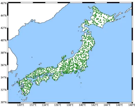
To estimate the non-linear site response, the usual practice is to use numerical simulations with equivalent linear analysis or truly non-linear time domain approach. In this document, we study the influence of the nonlinear soil behavior on the seismic site response by analyzing the earthquake recordings from borehole array configurations. We use the Kiban Kyoshin network (KiK-Net) data. All 688 sites are instrumented with two 3-components accelerometers, one located at the surface and the another at depth. From these data, we compute the ground motion amplifications from the surface to downhole recordings by the computing Fourier spectral ratios for the aim to compare between the spectral ratio for weak and strong ground motion.
The main effect of the non-linear behavior of the soil on the site transfer function is a shift of the amplification towards lower frequencies. We propose a new methodology to quantify those changes and study the nonlinear effects. This work results in a site-dependent relationship between the changes in the site response and the intensity parameter of the ground motion. The method is tested analyzing the records of the earthquake of Kumamoto (Mw 7.1, 2016).
Posteriorly, we propose to integrate a correlation between seismic moment and the duration of the fault
(Courboulex et al., 2016)
in the empirical Green’s function method. This methodology was applied to simulate one seduction event in Ecuador, and we compare the results with the records of the Pedernales earthquake (Mw 7.8, 2016) in the city of Quito.We attempt to take in account the nonlinear effects in the empirical Green’s function method. We use the methodologies of the first part of this document based on the frequency shift parameter. The procedure could be implemented in other methodologies that can predict an earthquake at a rock reference site, such as the stochastic methods. We test the procedure using the accelerometric records for one of the aftershocks o the Tôhoku earthquake (Mw 7.9).
Keywords: Earthquakes, Site effects, Non-linear soil behavior, Empirical Green Functions, Seismic risk, Japan, Ecuador
Acknowledgements
I am thankful with all the persons who were part of the process during those three years. I start with my director of the thesis, Etienne. Thanks for helping me since the beginning with all the initial problems that arriving France involved, as the security social, adapting process, between others. Also, thanks for being part of the thesis and always solving the questions and contribute ideas for developing this project. Thanks to Françoise, the co-director of the doctorate, because you explained me all the necessary to progress and to understand the seismology topic. I feel my understanding of seismology methods is one of the central learning I obtained during those years. Also, thanks Françoise for all the other aspects were your help was indispensable, as the administrative process at the end of the thesis and in my integration into the laboratory of GeoAzur. Thanks to Julie, the instructor of the thesis, for the discussions and all the knowledge you contributed to developing this thesis. I am thankful for all this group of work for the ideas, the energy, and the time you dedicated to this thesis. Equally, thank you very much for selecting me for this project and give the opportunity of research with you.
I want to thanks to the rapporteurs of this work, Cecile Corneau chargée de recherche at the laboratory of ISTerre, and the professor Fabrice Cotton of GFZ Potsdam by kindly accept to take part of your time to read and exanimate this document. Thanks for your constructive critics that made better this document.
I want to express my gratitude with the committee of the thesis, formed by Diego Mercerat of Cerema and Fernando Lopez-Caballero of Centrale Superlec, because in different opportunities they exanimated the progress of the thesis and also they gave me advice of how to improve the project. Thanks also to Fabian Bonilla-Hidalgo, and all the members of the jury for accepting come to Nice and be part of the defense of this thesis with the examination of this work. Thanks to all the team of Cerema, the place where I developed the thesis. They always give me great talks during those three years. Thanks, to the group of risky seismic Nathalie, Philippe, Michell and the new members of the seismic risk team Ophélie and Matthieu. I want to thanks to my office mate during the thesis, Simon, who always was available to solve any question and he gave me the initial encourage and essential knowledge for learning and developing all the computations in Python. Thanks also all the members of Cerema who help me in different aspects and they had the best disposition to make my place of work very comfortable. Thanks, Marie France, Dominique, Jean-Baptiste, Yannik, and all Cerema.
Thanks to the members of GeoAzur that comment and contribute to my work, and also teach me in different opportunities, thanks Maria-Paula, Jean-Paul, Bertrand, Jenny, Anthony, Cédric. Thanks to all the persons I shared time and made better those three years. Thanks Asmae, Edward, Hector, Huyen, Louisa, Nicholas S, Reine, Sadrac, and all. Also, thanks to many persons who commented on my work in different opportunities and gave me in some cases new ways to improve the work presented herein: Jean-François Semblat, Pierre Bard.
I am especially grateful with the persons that were with me during all those years, even with the distance. Thank very much to my family and friends that always they were there to support me.
Contents
Résumé ... i
Abstract ... ii
Acknowledges ... iii
Contents ... iv
Introduction ... 1
Chapter I
Theoretical verification of a new parameter to quantify the non-linear
soil behavior: the frequency shift parameter Dynamic soil response model ... 5
I.1 Linear site response ... 5
I.1.1 Soil response of a linear elastic soil layer on total rigid bedrock ... 5
I.1.2 Linear viscos-elastic soil on a rigid bedrock ... 9
I.1.3 Solution Multiple viscoelastic soil layers on an elastic bedrock ... 11
I.2 Non-linear soil response facing a dynamic solicitation ... 16
I.2.1 General characters of the non-linear behavior ... 16
I.2.2 Approximation with G/Gmax curves and damping curves... 18
I.2.3 Variation of the non-linear behavior due to different parameters ... 19
I.2.4 Hyperbolic model and non-linear soil characterization ... 21
I.2.5 Characterization of the soil materials: Damping and stiffness decay curves by cyclic triaxial test 21 I.3 Numerical implementation of the non-linear soil behavior ... 23
I.3.1 Method of the equivalent linear analysis (EQL) ... 23
I.3.2 Other non-linear models ... 24
I.4 Definition of a new parameter to quantify the loss of stiffness from spectral analysis ... 25
I.4.1 The parameter fsp: Analysis with the equivalent linear method ... 26
I.5 The parameter fsp: Fully non-linear model ... 29
I.6 Summary and discussion ... 32
Chapter II
Signal processing and Borehole arrays to study the non-linear behavior
of the soil
34
II.1 Borehole arrays ... 34II.1.1 Kik-net database ... 35
II.1.2 General statistics of Kik-Net database ... 37
II.2 Signal processing ... 39
II.2.1 Selection of the window of interest ... 39
II.2.2 Removing the mean ... 40
II.2.3 Applying the Hanning’s window ... 41
II.2.4 Addition of zero pad to the signal ... 43
II.2.5 Signal Process: Application of butter filter ... 43
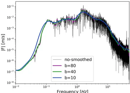
II.2.6 Spectrum processing: Konno-Ohmachi smoothing ... 45
II.3 Borehole spectra ratio (BSR) ... 46
II.4 Summary ... 47
Chapter III
Impact of the soil non-linear behavior on the seismic site response ... 48
III.1 Influence of the non-linearity of the soil in BSR ... 48
III.2 RSR definition and analysis of the amplitude differences ... 50
III.3 Frequency shift parameter (fsp) from signal records ... 51
III.3.1 Estimation of the linear site response (BSRlinear) ... 52
III.3.2 Computation of fsp parameter ... 53
III.3.3 Computation of fsp curves ... 55
III.4 Comparison of fsp and shear modulus reduction curves ... 56
III.5 Prediction of strong motion 2016 Kumamoto earthquake (Mw 7.1) ... 57
III.5.1 Methodology ... 57
III.5.2 Kumamoto earthquake and sites of analysis ... 58
III.5.3 Estimation of 𝐵𝑆𝑅 ... 62
III.5.4 Prediction of the amplitude of the Fourier spectrum at surface ... 64
III.5.5 Time history prediction ... 66
III.5.6 Prediction of the response spectra ... 68
III.6 Amplification decrease consideration ... 70
III.7 Predictions of the site effects using both fsp curves and ∆BSRISA. Application to 2016 Kumamoto earthquake, Mw 7.1 ... 76
III.7.1 Methodology ... 76
III.7.2 Estimation of BSR ... 77
III.7.3 Prediction of the Fourier spectrum at surface ... 82
III.7.4 Time history prediction ... 83
III.7.5 Prediction of the response spectra ... 85
III.8 Conclusion ... 87
Chapter IV
Evaluation of fsp on H/V spectral ratio ... 88
IV.1 Earthquake H/V spectral ratio technique ... 88
IV.2 A{H/V-linear} curve and fundamental frequency of the site, fo{H/V} ... 88
IV.3 Effects of the non-linearity on the curve of H/V ratio ... 92
IV.4 Analysis of fsp curves for all the whole database. ... 94
Chapter V
Analysis of the 𝒇𝒔𝒑 curves using site parameters. ... 99
V.1 Description of the 𝒇𝒔𝒑 curves at the kik-net sites ... 99
V.1.1 Variation of the 𝑓𝑠𝑝 curves from site to another ... 99
V.1.2 Description of the standard deviation to quantify the variation of 𝑓𝑠𝑝 curves at the kik-net sites 101 V.1.3 Selection of a sub-dataset ... 103
V.2 The relationship between fsp curves and site parameters ... 104
V.2.1 Analysis of the average shear wave velocity ... 104
V.2.2 Influence of the impedance contrast on fsp curves ... 106
V.2.3 Influence of the downhole device on the fsp curves ... 107
V.2.4 Relationship between the fundamental frequency, determined by the H/V ratio, and fsp curves. 108 V.3 fsp with different intensity parameters ... 109
V.3.1 Parameter: PGAsurface ... 109
V.3.2 PGVsurface/Vs30 ... 114
V.4 Summary and discussion ... 117
Chapter VI
Ground motion prediction using an Empirical Green’s Function method
constrained by a global database ... 119
VI.1 Source model (ω2-model) ... 119
VI.2 Effects of Mo, fc and Δσ in the spectrum of an earthquake following the ω2-model 121 VI.3 Empirical Green’s function method ... 124
VI.3.1 Criteria to use EGF method ... 128
VI.4 Relationship between corner frequency, seismic moment and stress drop ... 128
VI.5 Sensitivity analysis of EGF method facing the a stochastic duration of the fault .. 131
VI.6 Case of the Pedernales Mw 7.8 (Ecuador) Earthquake ok 16 April 2016 ... 133
VI.6.1 Signal processing and distance correction ... 136
VI.6.2 Determination of the corner frequency for each EGF ... 136
VI.6.3 Comparison in a blind test simulation ... 139
VI.7 Simulation of a Mw8.5 earthquake in Quito... 156
VI.8 Summary and discussion ... 163
Chapter VII
First attempt to the integration of non-linear site effects on the
Empirical Green Function methodology using borehole arrays ... 165
VII.1 Methodology of integration of non-linear effects by fsp curves and the EGF method. ... 165
VII.1 Ground motion prediction of an aftershock (Mw 7.9) of the 2011 Tohoku earthquake ... 166
VII.1.1 Application of the EGF method with linear site effects ... 166
VII.1.2 Comparison of the EGF simulation of the surface strong ground motion at FKSH10 with or without including non-linear effects ... 169
VII.2 Conclusion and discussion ... 172
Conclusions ... 173
Bibliography ... 176
Annex A.
Derivation of the equation for 1D wave in a viscoelastic media ... 190
Annex B.
Results of the Kumamoto simulation ... 201
Annex C.
Fsp curves ... 226
Introduction
Motions in the lithosphere occur at different time scales: from the very long geologic times for the plate tectonic to few seconds for fault ruptures. The fault ruptures produce earthquakes due to the sudden release of accumulated energy that is spread in the Earth in the form of seismic waves.
The number of earthquakes per year is estimated at more than one million (IRIS, 2011). About 10.000 of them reach a magnitude larger than 4 but they are unable to cause damage to the population. Strong earthquakes hopefully are less frequent, but they are able to strongly affect our societies causing several fatalities and big losses in the infrastructures. Moreover, the earthquakes can trigger landslides and tsunamis. Earthquake engineers try to anticipate and to prepare the infrastructure for mitigating the seismic risk. For this aim, the energy and the frequency of the seismic ground motions must be anticipated.
The ground motions are first related with the way the energy from the accumulated stress on a fault is released. These so-called source effects affect the ground motions and depend mainly on the moment released (that depends on the surface of the fault and the displacement of the fault), the rupture velocity, and the stress drop (difference of stress before and after an earthquake). Then, the seismic waves generated at the source are modified by their travel in the underground medium (so called path effect). Those effects cause a dissipation of the energy (geometrical and anelastic attenuation) and changes in the frequency content and waveforms, related with complex interactions between the seismic wave and the underground structure medium.
Finally, the site effects refer to the influence that superficial layers of soil have on the final surface ground motion. The Michoacan earthquake (M=8.5) that occurred in the city of Mexico in 1985 revealed the very strong amplification in ground motions recorded on the soft unconsolidated sediment of the basin compared with the recordings outside (e.g. Anderson et al., 1986; Singh et al., 1988). The ground motion amplifications due to superficial layers caused high damages and an impact on the building of the basin. Site effects are mainly caused by the last hundred meters of soil. The area where the site effects occur is very small in comparison with the path and source effects that can involve tens or hundreds of kilometers. The high influence of the site effects in the ground motions has been detected for many other cities (e.g. Fleur et al., 2016; Laurendeau et al., 2017; LeBrun et al., 2001). The current building codes implement the site effects in different grades to manage the seismic risk of the infrastructure. The main causes of the site effects are the strong changes in the mechanical properties of the soil close to the surface. The changes of stiffness make that the energy gets trapped in the last layers of soil, causing for some frequencies constructive interferences at the surface creating a strong amplification of the ground motion.
Furthermore, the shear modulus and the damping are dependent on the amplitude of the seismic wave that travels across the shallow soil layers. It changes the soil response of strong events with respect to weak events. This phenomenon, often called non-linear effect were first detected in seismic events comparing the modeled linear soil response with the real ones from 1957 San Francisco earthquake at several sites (Idriss and Seed, 1968). After this, using many methodologies other works have detected the soil non-linearity in seismic records. For example,
comparing the site response between strong and weak events the non-linear effects were detected in the earthquake of Mexico Mw 8.5 (Singh et al., 1988) and for the earthquake of Loma and Pieta Mw 6.9 in United States (Aki, 1993; Beresnev and Wen, 1996; Darragh and Shakal, 1991). After them, the non-linearity have been interpreted in seismograms as a reduction in the amplification at high frequencies and in some cases an increasing of the amplification at low frequencies (e.g. Bonilla et al., 2011; Régnier et al., 2016b; Sawazaki et al., 2006). Another usual way to evaluate the soil non-linearity is through proxies to estimate the stress and the strain of the soil column (e.g. Bonilla et al., 2005; Zeghal and Elgamal, 1994). In the recent years, using methods of interferometry the time that the wave takes between two points is estimated and by this the shear modulus decay is evaluated (e.g. Bonilla et al., 2017; Chandra et al., 2015; Nakata and Snieder, 2012; Sawazaki et al., 2009).
As was mentioned, the task of prediction of the seismic ground motion involves the source, path and site effects, and it is very important in the earthquake engineering. This task has been addressed by many methodologies, in some cases with numerical simulations or with empirical evaluations. For example, one empirical approach used to predict ground motion for engineering needs is the use of Ground motion prediction equation (GMPEs). GMPEs are equations build from large database of real ground motions recorded over the world (e.g. Douglas, 2011, for a review). They enable to predict a mean value and a variability of the ground motions given simple parameters like magnitude, distance and a site parameter often based on the mean shear wave velocity of the first 30 meters of soil (Vs30). GMPES are very powerful tools
to predict ground motions parameters in general cases. The drawback of this method is the high uncertainty associated with the inclusion of different earthquakes from different regions and conditions in the analysis. It implies, for example, that important individual conditions as the site effects and the soil non-linear behavior are not taken into account.
Numerical methods are also used to attempt modeling the earthquake phenomena. These analyses employ numerical approximations that involve different complexities depending of the model. Most of them reduce the geometry to one dimension, although some of them evaluate the three components of the motions. Other kind of numerical models involve two or the three dimensions of the space. The definition of the materials in the numerical models is an essential part for the performance of the prediction of the ground motions. Often the models assume that the materials are linear. In other cases, the soil models introduce the non-linearity by relating the soil behavior with several rules that relate the soil properties with the state of the material (e.g. Iwan, 1967; Masing, 1926). These methodologies require input parameters that are complex to estimate and measure, like the geometry of deeper layers, and stiffness and damping of all the involved materials in the media. This definition of parameters brings a high cost, regarding the time and work, and also has a high uncertainty associated. Additionally, numerical models have a high uncertainty in their results due to the constitutive model and the measurement of non-linear parameters (Régnier et al., 2018).
Another alternative is the simulation by empirical methods. One of the examples is the empirical Green functions approach (EGF). It extrapolates weak seismic motions available in our databases to stronger motions. This method includes the source effects, path effects, and site effects. The method is also widely used because it does not require specific information as the geometry and the soil characteristics to well predict a future strong earthquake. One of the biggest complications that this methodology has is its dependence on the stress drop of the future earthquake. This dependence makes the methodology hard to be applied since it is not easy to determinate this parameter for an earthquake that has not occurred yet.
Another limitation of the EGF method is the assumption that all earthquake system is propagating in a medium characterized by linear behavior. It means that the evaluation does not considers the non-linear behavior of the shallow soil layers. This is also an important issue in most of the methodologies to simulate ground motions, not just EGF method, as stochastic methods (e.g. Boore, 2003), and GMPE formulas.
The non-linear soil effects can be a major aspect of the strong ground motion prediction. The role of the non-linear soil behavior on the seismic motion makes it important for seismic hazard assessments.
In summary the quantification and the consideration of the effects of the non-linear soil behavior is an important aspect that we study in this document.
Objectives
In the work presented here, we aim to evaluate the non-linearity of the shallow soil layers with an empirical methodology. We search to evaluate and to quantify the effects that the non-linearity has on the seismic response of the soil. This analysis is done by studying the site response in function of the level of seismic solicitation. We use results coming from borehole spectral ratio (BSR) and from earthquake H/V spectral ratio computations.
We propose an empirical methodology to predict the non-linear soil behavior effects on site response that can be used to include the non-linearity in other methodologies of earthquake estimation, as EGF method. This proposition will allow to better predict strong ground motions, especially for countries with low seismicity where only weak to moderate earthquake recordings are available.
We also aim to solve the limitation of applicability for the EGF method. We will introduce in the methodology of Kohrs-Sansorny et al., (2005) a procedure to manage the variability given by the estimation of the stress drop. This procedure will be based on the analysis of the fault duration with the seismic moment (Courboulex et al., 2016), transforming the fault duration regarding the stress drop.
Outline
• Chapter I of this document presents the theoretical background to quantify and to analyze the site effects by computing the transfer function of a soil column. We present the influence of aspects as the damping, the impedance, and the bedrock by the changes that they generate on the transfer function. A new parameter called fsp quantifies the effect of the loss of stiffness of the soil in the transfer function. Using the equivalent linear method and a full non-linear method we test the theoretical relevancy of the fsp parameter under complex conditions.
• Chapter II presents the signal processing that is applied to the earthquake recordings in this work. Subsequently, Chapter II presents the borehole arrays configurations that are used to analyze the site effects.
• Chapter III presents a procedure to quantify the level of non-linearity on the sites during a strong ground motion. The procedure is based on the fsp parameter, using records
from vertical arrays. This parameter focuses in the measure of the stiffness degradation that the soil suffers. It shows a link between fsp and the modulus reductions curve. Using fsp, we present a methodology to estimate the site response for future strong ground motions. Also, analyzing the trend of several records, a methodology that estimates the decrease of the site effects amplification is shown.
• Chapter IV presents a methodology to estimate the non-linearity influence on the site response using earthquake H/V spectral ratio technique. This methodology uses again the fsp parameter, and a comparison with the estimation using borehole arrays is presented.
• Chapter V presents a statistical analysis of the results on all kik-net database. This analysis presents relationships between site parameters, as Vs30 and fundamental
resonance frequency, with the propensity of a site to develop non-linear behavior, defined by fsp curves.
• Chapter VI shows a new procedure to use the EGF method estimating the stress drop of the future earthquake. This methodology also manages the variability associated with the stress drop estimation, having results comparable with the most advanced GMPE methods. However, EGF method can estimate better the site effects, producing more realistic response spectra than the general shape of the GMPE methods.
• Chapter VII presents a first attempt of the integration of the non-linear soil behavior, based on the fsp parameter correction, in the EGF approach.
Chapter I Theoretical verification of a new
parameter to quantify the non-linear soil
behavior: the frequency shift parameter
Dynamic soil response model
In this chapter we introduce the analytical and numerical evaluation of seismic site response (lithological site effects) for the shear waves propagating in a unidimensional medium with a vertical incidence and the estimation of the site response. The linear elastic and visco-elastic soil behavior are first analytically analyzed and then, the non-linear soil behavior is introduced through numerical modeling. The impact of the various hypothesis on the soil behavior is observed on the site response (transfer function of the site).
With the help of this mathematical development, the theoretical relevancy of a new parameter, to quantify the impact of the non-linear soil behavior on site response, is discussed. The new parameter, called fsp for frequency shift parameter, quantifies one of the main effects of the soil non-linear behavior which is the decrease of the shear modulus during strong motion.
I.1 Linear site response
For sake of clarity, we decided to begin with the presentation of the seismic wave propagation in the simplest site configuration cases. We consider no lateral variability of the soil (one-dimension assumption) and the propagation of seismic shear waves only with a vertical incidence. In addition, the soil model used involves first a unique layer of soil underlined by a rigid rock substratum and then we will consider a multilayer of soil model with an elastic substratum.
In this section, the transfer functions between the bedrock and the surface are presented for several soil constitutive models (elastic, viscoelastic).
The 1-D assumption is not adequate for sites with complex site configurations such as a deep and narrow valleys (like Alpine valley). In the next sections, we explain briefly the 2-D and 3-D modeling. However, the vertical incidence of the wave is an assumption that is accomplished if the hypocenter of the earthquake is deep and far enough from the site investigated. It is because the direction of propagation of the waves is modified by passing from one layer of soil to another when the stiffness of soil differs. Since the stiffness of the soil decrease from the depth to the surface (especially the few hundred meters of soil) the waves will reach the surface with approximately a vertical incidence.
I.1.1 Soil response of a linear elastic soil layer on rigid bedrock
This section analyzes a model that consists in one layer of soil lying on a total rigid rock with vertical shear waves propagating with vertical incidence (Figure I-1).
Figure I-1. Sketch of the motel of soil that is overlying a bedrock. H and Vs represent the thickness and the shear velocity of the ground.
In the Figure I-1, H represents the thickness of the soil layer, Vs is the shear wave velocity, which is linked with the rigidity of the material. To analyze the propagation of a shear wave in this model, we can start from the motion equation that is required to be accomplished at any place of the model by the dynamic equilibrium (second Newton’s law) express as:
𝜌𝜕
2𝑢
𝜕𝑡2 =
𝜕𝜏
𝜕𝑧 (I-1)
Where u represents the horizontal displacement, t is the time, ρ is the density, z is the depth, and τ represents the shear stress. Since the model is in one dimension, the equation considers lateral displacement and shear stress traveling in the unique dimension.
If the material has no damping (ξ=0) the relationship between the shear stress and strains (γ=∂u/∂z) is linear. In this case, the soil can be modeled trough the Hooke’s law (Eq. (2)).
𝜏 = 𝐺𝜕𝑢
𝜕𝑧 (I-2)
Where G represents the shear modulus and du/dz is the shear strain. The shear strain is a measure of the distortion of the material.
Introducing this equation (Eq. (I-2)) to the motion equation (Eq. (I-1)), the wave equation is obtained (Eq. (I-3)):
𝜕2𝑢 𝜕𝑡2 = 𝑉𝑠
2𝜕2𝑢
𝜕𝑧2 (I-3)
Where Vs is the shear velocity defined as:
𝑉𝑠= √𝐺 𝜌⁄ (I-4)
For this solution we suppose that only a mono frequential periodic wave is travelling by the media. However, from this solution the result for another kind of inputs can be also computed, as we will explain hereunder. In this case, the general solution for the Eq. (I-3) has the shape:
𝑢(𝑧, 𝑡) = 𝐴 ∙ 𝑠𝑖𝑛(𝛼(𝑉𝑠𝑡 − 𝑧) + 𝜑) + 𝐵 ∙ 𝑠𝑖𝑛(𝛼(𝑉𝑠𝑡 + 𝑧) + 𝜑)
Where A, B, φ, and α are constants that will be defined with the boundaries conditions of each problem. The previous equation has two terms. Physically, the first term with amplitude A represents the upwards waves and the other the downwards waves.
In a soil column with 1D propagation, at the surface the shear stress cannot be developed. It implies that at the surface (z=0, see Figure I-1) the shear stress cannot be generated:
𝜏(𝑧 = 0) = 0 𝑡ℎ𝑒𝑛𝜕𝑢
𝜕𝑧(𝑧 = 0, 𝑡) = 0 (I-5)
At the bedrock, like at surface, stresses are imposed. This stress is in function of the input wave. We first consider a periodic function with a unique frequency as an input motion (Eq. (I-6)).
𝜏(𝑧 = 𝐻) =𝜕𝑢
𝜕𝑧𝐺 = 𝜏𝑜∙ sin(2𝜋𝑓𝑡 + 𝜑𝑙) (I-6)
Where τo is the stress wave amplitude, φl is the phase of the loading wave, and f is the frequency
associated with the wave. In Annex A the mathematical solution with trigonometric expressions is developed for solving the wave equation (Eq. Eq. (I-3)) under the boundary conditions previously expressed. The general solution of the problems arrives is:
𝑢(𝑧, 𝑡) = 2𝐴 ∙ sin(2𝜋𝑓𝑡 + 𝜑𝑙) cos(2𝜋𝑓𝑧/𝑉𝑠) (I-7)
In the previous expression A is a constant value. In some cases, the last equation is presented in function of the angular frequency ω=2πf and the wave number k= ω/Vs which give the final
solution:
𝑢(𝑧, 𝑡) = 2𝐴 ∙ sin(𝜔𝑡 + 𝜑𝑙) cos(𝑘𝑧)
The solution to the wave equation (I-7) depends on the frequency of the input wave. The transfer function between two locations, represented by the ratio between the displacements at the two locations, indicate the way the waves changes from one point to another. To study the site effects, we evaluate the displacements at the surface and at the bottom of the soil layer on the bedrock. The ratio is computed as:
𝑇𝐹{0/𝐻}(𝑓) = 𝑢(0, 𝑡) 𝑢(𝐻, 𝑡)= 2𝐴 ∙ sin(2𝜋𝑓𝑡 + 𝜑𝑙) cos(2𝜋𝑓0/𝑉𝑠) 2𝐴 ∙ sin(2𝜋𝑓𝑡 + 𝜑𝑙) cos(2𝜋𝑓𝐻/𝑉𝑠) 𝑇𝐹{0/𝐻}(𝑓) = 1 cos(2𝜋𝑓𝐻/𝑉𝑠) (I-8)
The formula (I-8) shows that the amplification given by the site depends on the frequency. For some frequencies the amplification tends to infinite because the denominator can be equal to zero. It occurs when the term inside the cos function is equal to 𝜋(0.5 + 𝑛) , where n is any integer number.
𝑓{𝑛}= 𝑉𝑠
2H(0.5 + 𝑛) 𝑓𝑜𝑟 𝑛 = 0, 1, 2, … (I-9)
Where f{n} is the nth frequency peak that is amplified by the site. Those frequencies are called
resonance frequencies. This phenomenon occurs because the input wave enters into constructive interference with the downwards waves that have been reflected at the free surface. This together with the hypothesis that the bedrock is rigid and that the soil is undamped, meaning that the energy cannot escape from the ground, make that the amplifications for those frequencies tend to infinite.
The first peak of the transfer function (f{0}) is called the fundamental resonance frequency, and
is often used to characterize the soil columns (e.g. Luzi et al., 2011).
To study the amplification in other frequencies, the transfer function in Figure I-2 represents the amplification for a general case. The amplification is shown for any soil model with fixed H and Vs.
Figure I-2. Transfer for an elastic undamped layer of soil on a total rigid bedrock.
In a more realistic case, the input wave is not as simple as the Eq. (I-6). However, any function can be represented and discomposed as a summation of sinusoidal harmonic functions (Serie of Fourier, Fourier, 1822): 𝑢(𝐻, 𝑡) = ∫ 2|𝑈(𝐻, 𝑓)| sin (2𝜋𝑓𝑡 + arctan(−𝑅𝑒(𝑈(𝐻, 𝑓)) 𝐼𝑚(𝑈(𝐻, 𝑓)) ) 𝑑𝑓 ∞ 0 (I-10)
Where u(H, t) is the input wave, Re and Im are the functions to obtain the real and the imaginary part of a complex number respectively. The frequency depended function U(H, f) was defined by Jean-Batiste Joseph Fourier (1768-1830) as:
𝑈(𝐻, 𝑓) = ∫ 𝑢(𝐻, 𝑡) ∙ 𝑒−2𝜋𝑖𝑓𝑡𝑑𝑡
∞ −∞
(I-11)
Where U(H,f) is the Fourier transform of u(H,t), also call Fourier spectrum. Note that this transform applies for any function and it could be computed at any depth U(z,f).
The superposition principle applies for any linear system (as the Eq. (I-3)), and the solution of a composed input is equal to the summation of the solution for each part of the input. With the Fourier’s methodology (Eq. (I-10)) we can decomposed the input wave into sine functions with different frequencies, each one with the shape of the Eq. (I-6). Always that the phase (φl)
between both points is the same, we know that the solution for each part of the input has the same formulation than the previously obtained (I-7).
Applying the superposition principle, with the transfer function and the spectrum of the input wave, the spectrum of the ground motion at the surface can be computed as follow:
𝑈(0, 𝑓) = 𝑈(𝐻, 𝑓) ∙ 𝑇𝐹{0−𝐻}(𝑓) (I-12)
Where TF is the transfer function of the system (Eq. (I-8)), U(H,f) is the spectrum of the incoming wave, and U(0,f) is the spectrum at the surface. Because Eq. (I-12) is in the frequency domain, the operation is called the convolution between TF and u(H,t).
Finally, to compute the temporal response at the surface, the inverse transform of Fourier is applied. Already in the Eq. (I-10) was shown the formula for this transform, but usually, this transform is written in his exponential way as:
𝑢(𝑧, 𝑡) = ∫ 𝑈(𝑧, 𝑓) ∙ 𝑒2𝜋𝑖𝑓𝑡𝑑𝑓 ∞
−∞
(I-13)
With the previous equation, we can find the solution u(0,t) with U(0,f). It is important to note that using the Eq. (I-12) we are assuming that the phase is the same at all locations. This assumption is very well known in seismology, and many cases consider the phase even equal to zero (e.g. Brax et al., 2016; Robinson, 1967, 1957).
I.1.2 Linear viscos-elastic soil on a elastic bedrock
All the realistic soils dissipate energy. This dissipation of energy is associated with the pore water viscosity, interparticle friction, and particles rearrangement. This phenomenon is introduced into the strain-stress relationship, making the response shear stress of the material proportional to the rate of the shear strain. This effect, called damping, is implemented in the model presented in the previous subsection. The effect of implementing the damping on the transfer function is evaluated in this subsection.
An element that produces a stress proportional to the rate of strain is known as a damper. An element that produces a stress proportional to the strain and dominated by the Hooke’s law (Eq. (I-2)) is a spring. Mixing both elements, we obtain the physical representation of the viscos-elastic behavior.
In seismology, the configuration of Voigt-Kelvin is widely used. A material with this constitutive model has a hysteric behavior, with reversible strains. In this constitutive model, the stress that a material produces facing an imposed strain is dominated by the strain amplitude and rate (Eq. (I14)). 𝜏 = 𝐺𝜕𝑢 𝜕𝑧+ 𝜂 𝜕(𝜕𝑢𝜕𝑧) 𝜕𝑡 ⁄ (I-14)
Where η and G represent the viscosity and stiffness of the material. This model cannot be used to model permanent strains under zero stress, since it tends to zero after that the load has been removed and the rate of the strain is zero. Another limitation is that in this case the failure of the material never occurs.
Introducing the constitutive model of Voigt-Kelvin (Eq. (I-14)) instead of the Hooke’s law (Eq. (I-2)) in the motion equation (Eq. (I-1)), a new solution can be found, with a new differential equation that dominate the problem:
𝜌𝜕 2𝑢 𝜕𝑡2 = G 𝜕2𝑢 𝜕𝑧2+ 𝜂 𝜕3𝑢 𝜕𝑧2𝜕𝑡 (I-15)
The Eq. (I-15) is a linear partial differential equation. The boundary conditions of this problem are the same Eq. (I-5) and (I-6). Because the new equation that dominates the problem (Eq. (I-15)) is linear, it implies that like in the elastic case, we can calculate the transfer function. The mathematical development of these equations can be found in the Annex A. The general solution for a linear partial differential equation (Eq. (I-15)) is:
𝑢(𝑧, 𝑡) = (𝐶𝑒𝑖𝑘∗𝑧+ 𝐷𝑒−𝑖𝑘∗𝑧) ∙ 𝑒𝑖2𝜋𝑓𝑡+𝜑𝑙
(I-16)
Where C and D are constants that are defined with the boundary conditions and represents the upwards and downward waves amplitude respectively. In the solution a new wave number is defined as:
𝑘∗2=4𝜋2𝑓2𝜌⁄(𝐺 + 2𝜋𝑓𝜂𝑖) (I-17)
In the damped layer model, this number is complex. The solution of the previous equations is: 𝑢(𝑧, 𝑡) = 2𝐶 ∙ cos (𝑘∗𝑧) ∙ 𝑒𝑖2𝜋𝑓𝑡+𝜑𝑙
Where C is a constant. With the previous definition of u(z,t), we define de displacement at z=0 and z=H and the ratio gives the transfer function as:
𝑇𝐹{0/𝐻}(𝑓) = 𝑢(0, 𝑡) 𝑢(𝐻, 𝑡)= 2𝐶 ∙ cos(𝑘∗∙ 0) ∙ 𝑒𝑖2𝜋𝑓𝑡+𝜑𝑙 2𝐶 ∙ cos(𝑘∗∙ 𝐻) ∙ 𝑒𝑖2𝜋𝑓𝑡+𝜑𝑙 𝑇𝐹{0/𝐻}(𝑓) = 1 cos (2𝜋𝑓𝐻√𝜌⁄(𝐺 + 2𝜋𝑓𝜂𝑖))
Here a new term is introduced: ξ referred as the damping ratio coefficient of the material and it is defined as:
𝜉 =𝜋𝑓𝜂 𝑉𝑠2𝜌
⁄ (I-18)
Using the damping ratio coefficient (ξ) and introducing the definition of the stiffness in terms of shear velocity (G=Vs2ρ), it reduces the transfer equation to:
𝑇𝐹{0/𝐻}(𝑓) =
1 cos (2𝜋𝑓𝐻𝑉
𝑠 √1 (1 + 2𝜉𝑖)⁄ )
(I-19)
The function (I-19) is the formal definition of the transfer function for a damped layer on a total rigid bedrock. However, assuming that ξ is small enough (see Annex A) the previous function can be reduced even more to:
|𝑇𝐹{0/𝐻}(𝑓)| = 1 √cos2(2𝜋𝑓𝐻 𝑉𝑠 ⁄ ) + sinh2(𝜉2𝜋𝑓𝐻 𝑉𝑠 ⁄ ) (I-20)
The transfer function with damping (I-20) makes a difference with respect to the transfer function with elastic case (I-8). The amplitude at the resonance frequencies do not go to infinite since the denominator is never equal to zero (if the term inside the hyperbolic sine is not null (ξ>0)). However, the frequencies with maximal amplification are similar to the elastic case defined by the same Eq. (I-9).
Analyzing the amplification for all the frequencies in the damped system (Figure I-3), the transfer function does not exhibit peaks that tend to infinite in any resonance frequency. Additionally, the amplification for high frequencies are lower than the amplification for low frequencies. Increasing the damping makes the amplification lower (Figure I-3). If the damping is high enough, at high frequencies the peaks cannot be distinguished anymore and even the transfer function can take values lower than one, meaning that the site effect is reducing the input wave amplitude.
Figure I-3. Transfer function for a damped layer on a totally rigid bedrock. For example, the used layer had 5% damping.
Because the differential equation for the model (Eq. (I-14)) is a linear differential equation, the system for any input can be solved by the summation of the results for each part of the input. The procedure is the same than the one explained in the last subsection ((I-11), (I-12), Eq. (I-13)).
I.1.3 Solution Multiple viscoelastic soil layers on an elastic bedrock
In this subsection, we analyze (1) the modifications of the wave due to the traveling from one layer of soil to another is studied and (2) that the substratum is elastic. Similar hypothesis is considered concerning the behavior of the soil, linear viscoelastic with shear waves propagating with vertical incidence.
The multiple layering and the elasticity of the bedrock creates an important effect in the transfer function that is found analytically. The bedrock in this model is not infinitely rigid, therefore, part of the energy in the downwards waves is transmitted to the bedrock, and another part is reflected in the layers of soil. This effect makes that part of the energy can leave the model. For solving this system, we must define a new coordinate system for each layer of soil and the bedrock (Figure I-4). Zero of the local coordinate systems is the upper point of each the layer, and H{m} the bottom point of each layer.
Figure I-4. Model of one damped layer lying on an elastic bedrock (left) and an outcrop (rigth). Each layer has a local coordinates system.
The soil layers (Figure I-4) are visco-elastic in this model and they are controlled by the Eq. (I-15). The bedrock is elastic (Eq. (I-3)). Because both equations of motion are linear, the methodology to solve this problem will follow the same procedure as the previous subsections. For each layer we define a transfer function that link the movement from one point to the other of the same layer of soil.
In this case, more solution functions must be found, one by layer. However, the general solution for all the layer has the shape of the function (I-16), because it is solved for a harmonic input:
𝑢{1}(𝑧{1}, 𝑡) = (𝐴{1}𝑒𝑖𝑘{1} ∗ 𝑧 {1}+ 𝐵 {1}𝑒−𝑖𝑘{1} ∗ 𝑧 {1}) ∙ 𝑒𝑖2𝜋𝑓𝑡 𝑢{2}(𝑧{2}, 𝑡) = (𝐴{2}𝑒𝑖𝑘{2} ∗ 𝑧 {2}+ 𝐵 {2}𝑒−𝑖𝑘{2} ∗ 𝑧 {2}) ∙ 𝑒𝑖2𝜋𝑓𝑡 … 𝑢{𝑚}(𝑧{𝑚}, 𝑡) = (𝐴{𝑚}𝑒𝑖𝑘{𝑚} ∗ 𝑧 {𝑚}+ 𝐵 {𝑚}𝑒−𝑖𝑘{𝑚} ∗ 𝑧 {𝑚}) ∙ 𝑒𝑖2𝜋𝑓𝑡 … 𝑢{𝑏}(𝑧{𝑏}, 𝑡) = (𝐴{𝑏}𝑒𝑖𝑘{𝑏} ∗ 𝑧 {𝑏}+ 𝐵 {𝑏}𝑒−𝑖𝑘{𝑏} ∗ 𝑧 {𝑏}) ∙ 𝑒𝑖2𝜋𝑓𝑡 (I-21)
Where k*{m} is the wave number (Eq. (I-17)) and A{m} and B{m} are constants to be defined with
the boundary conditions. The other terms are explained inFigure I-4. Those solutions for each layer must accomplish the wave equation (Eq. (I-1)). The boundary conditions are the same (Eq. (I-5) and Eq. (I-6)), meaning that at the surface the shear stress is zero. In addition, the displacement and the stress must be equal at the interfaces of each layer. It guaranties the continuity of the solution in the model (Eq. (I-22)).
𝑢{𝑚}(0, 𝑡) = 𝑢{𝑚−1}(𝐻𝑚−1, 𝑡)
𝜏{𝑚}(0, 𝑡) = 𝜏{𝑚−1}(𝐻𝑚−1, 𝑡)
(I-22)
Solving the wave equation with the previous conditions, the constants A{m} and B{m} of each layer
𝐴{𝑚} =(𝐴{𝑚−1}𝑒 𝑖𝑘{𝑚−1}∗ 𝐻{𝑚−1}(1 + 𝛼 {𝑚−1}∗ ) + 𝐵{𝑚−1}𝑒−𝑖𝑘{𝑚−1} ∗ 𝐻 {𝑚−1}(1 − 𝛼 {𝑚−1}∗ )) 2 ⁄ 𝐵{𝑚} =(𝐴{𝑚−1}𝑒 𝑖𝑘{𝑚−1}∗ 𝐻{𝑚−1} (1 − 𝛼{𝑚−1}∗ ) + 𝐵{𝑚−1}𝑒−𝑖𝑘{𝑚−1} ∗ 𝐻 {𝑚−1}(1 + 𝛼 {𝑚−1}∗ )) 2 ⁄ (I-23)
The mathematical development of the previous equation is shown in the Annex A. In the previous equation a new variable is defined to characterize the interface between two layers with the impedance (α). The impedance (α) is defined as the ratio between the apparent stiffness of the top layer and the stiffness of the lower layer.
𝛼{𝑚−1}∗ =𝐺{𝑚−1}(1 + 2𝜉{𝑚−1}𝑖)𝑘{𝑚−1}
∗
𝐺{𝑚}(1 + 2𝜉{𝑚}𝑖)𝑘{𝑚}∗
(I-24)
To find the transfer function between waves at the surface of an outcrop rock (z{0}=0, Figure I-4), and at the top of the soil layers (z{1}=0, Figure I-4), we obtained:
𝑇𝐹{0/𝑜𝑢𝑡𝑐𝑟𝑜𝑝}(𝑓) = 𝑢{1}(0, 𝑡) 𝑢{𝑜}(0, 𝑡) =2𝐴{1}∙ 𝑒 𝑖2𝜋𝑓𝑡 2𝐴{𝑏}∙ 𝑒𝑖2𝜋𝑓𝑡
Including the Eq. (I-23) in the previous one:
𝑇𝐹{0/𝑜𝑢𝑡𝑐𝑟𝑜𝑝}(𝑓) = 2 ∙ 𝐴{1} (𝐴{𝑛}𝑒𝑖𝑘{𝑛}∗ 𝐻{𝑛}(1 + 𝛼 {𝑛}∗ ) + 𝐵{𝑛}𝑒−𝑖𝑘{𝑛} ∗ 𝐻 {𝑛}(1 − 𝛼 {𝑛}∗ )) ⁄ (I-25)
Transforming the previous equation again, by replacing the coefficients A{n} and B{n} with Eq.
(I-23): 𝑇𝐹{0/𝑜𝑢𝑡𝑐𝑟𝑜𝑝}(𝑓) = 4 ∙ 𝐴{1} ( 𝐴{𝑛−1}𝑒𝑖(𝑘{𝑛} ∗ 𝐻 {𝑛}+𝑘{𝑛−1}∗ 𝐻{𝑛−1})(1 + 𝛼 {𝑛}∗ )(1 + 𝛼{𝑛−1}∗ ) + 𝐵{𝑛−1}𝑒𝑖(𝑘{𝑛} ∗ 𝐻 {𝑛}−𝑘{𝑛−1}∗ 𝐻{𝑛−1})(1 + 𝛼 {𝑛}∗ )(1 − 𝛼{𝑛−1}∗ ) + 𝐴{𝑛−1}𝑒𝑖(−𝑘{𝑛} ∗ 𝐻 {𝑛}+𝑘{𝑛−1}∗ 𝐻{𝑛−1})(1 − 𝛼 {𝑛}∗ )(1 − 𝛼{𝑛−1}∗ ) + 𝐵{𝑛−1}𝑒𝑖(−𝑘{𝑛} ∗ 𝐻 {𝑛}−𝑘{𝑛−1}∗ 𝐻{𝑛−1})(1 − 𝛼 {𝑛}∗ )(1 + 𝛼{𝑛−1}∗ ) ) ⁄
Recurrently the terms A{m} and B{m} could be replaced with the Eq. (I-23) by their predecessor A{m-1} and B{m-1} until the first layer. The final formula is expanding, and the general solution is:
|𝑇𝐹
{𝑜𝑢𝑡𝑐𝑟𝑜𝑝0 }(𝑓)| = 1⁄|𝑐(𝑘{𝑛}∗ 𝐻{𝑛}, … , 𝑘{1}∗ 𝐻{1}, 𝛼{𝑛}∗ , … , 𝛼{1}∗ )| (I-26)
Where c is the combination of exponential functions obtained from recurrently replacing the coefficients (Eq. (I-23) in the Eq. (I-25)). The wave number (k{m}) is defined in the Eq. (I-27), the
thickness of each layer (H{m}) depends on each case, and the impedance (α{m}) for each layer is
defined in the Eq. (I-24) (see Annex A for the mathematical developing of this formula). The wave number of each layer(k*{m}) can be also defined in terms of the damping and shear velocity
replacing the Eq. (I-18) and Eq. (I-4) in the Eq. (I-17):
𝑘{𝑚}∗ = 2𝜋𝑓 𝑉𝑠{𝑚}√
1 1 + 2𝜉{𝑚}𝑖
Assuming that the damping ratio is small enough (see Annex A for more details), in a first order of approximation, it allows to rewrite the square root term in the wave number as:
𝑘{𝑚}∗ ≈ 2𝜋𝑓
𝑉𝑠{𝑚}(1 − 𝜉{𝑚}𝑖) (I-27)
Using the same procedure, but this time involving the downwards waves, the transfer function between any layer interface and the surface (borehole transfer function) can be found as:
𝑇𝐹{0/𝐻{𝑚}}(𝑓) = 𝑢{1}(0, 𝑡) 𝑢{𝑚}(0, 𝑡) = 2𝐴{1}∙ 𝑒 𝑖2𝜋𝑓𝑡 (𝐴{𝑚}+ 𝐵{𝑚}) ∙ 𝑒𝑖2𝜋𝑓𝑡
Using the Eq. (I-23) in the previous equation: 𝑇𝐹{0/𝐻{𝑚}}(𝑓) = 2𝐴{1} (𝐴{𝑚−1}𝑒 𝑖𝑘{𝑚−1}∗ 𝐻{𝑚−1}(1 + 𝛼 {𝑚−1}∗ ) + 𝐵{𝑚−1}𝑒−𝑖𝑘{𝑚−1} ∗ 𝐻 {𝑚−1}(1 − 𝛼 {𝑚−1} ∗ ) + 𝐴{𝑚−1}𝑒𝑖𝑘{𝑚−1} ∗ 𝐻 {𝑚−1}(1 − 𝛼 {𝑚−1}∗ ) + 𝐵{𝑚−1}𝑒−𝑖𝑘{𝑚−1} ∗ 𝐻 {𝑚−1}(1 + 𝛼 {𝑚−1}∗ ) ) Reducing to: 𝑇𝐹{0/𝐻{𝑚}}(𝑓) = 𝐴{1} (𝐴{𝑚−1}𝑒𝑖𝑘{𝑚−1}∗ 𝐻{𝑚−1}+ 𝐵 {𝑚−1}𝑒−𝑖𝑘{𝑚−1} ∗ 𝐻 {𝑚−1}) ⁄
The previous equation shows that in the borehole transfer function, even if the recording device is located at interface of the layer, the impedance of deeper layers (for example 𝛼{𝑚−1}∗ ) does not affect the transfer function.
Replacing recurrently the Eq. (I-23) to move from A{m} and B{m} until A{1} and B{1}, that are equal
because of the free surface conditions, the absolute value of the transfer function is:
|𝑇𝐹{0/𝐻}(𝑓)| = |1 𝑑(𝑘
{𝑚}∗ 𝐻{𝑚}, … , 𝑘{1}∗ 𝐻{1}, 𝛼{𝑚−2}∗ , … , 𝛼{1}∗ )
⁄ | (I-28)
Where d is a combination of exponential functions, but in this case, it involves the parameters of the layers until the layer m. Additionally, it involves the downwards waves.
Using the Eq. (I-26), it is possible to find the movement at the surface due to any input wave, as was explained in the equations (I-11), (I-12) and (I-13). After, using movement at the surface, by the Eq. (I-28), the displacement for any interface point can be found, using also the inverse Fourier transform (Eq. (I-11), Eq. (I-12) and Eq. (I-13)).
To analyze the influence of the impedance contrast on the transfer function a simple case is evaluated. It consists in a monolayer model with the same characteristics of the previous subsection, but with an elastic bedrock with a finite stiffness is evaluated (Figure I-5).
Figure I-5. Sketch of the model of soil that is overlying an elastic bedrock. H, ξ and Vs represent the thickness, the damping, and the shear velocity of the ground.
Considering one layer of soil, using the Eq. (I-26) the transfer function would result in:
|𝑇𝐹 {𝑜𝑢𝑡𝑐𝑟𝑜𝑝0 }(𝑓)| = 2 |𝑒𝑖𝑘{1}∗ 𝐻{1}(1 + 𝛼 {1}∗ ) + 𝑒−𝑖𝑘{1} ∗ 𝐻 {1}(1 − 𝛼 {1}∗ )| ⁄
Reordering the previous expression and applying Euler properties and the expression of the wave number k* in the Eq. (I-27):
|𝑇𝐹 {𝑜𝑢𝑡𝑐𝑟𝑜𝑝0 }(𝑓)| = 1 √cos2(2𝜋𝑓 𝑉𝑠{1}(1 − 𝜉{1}𝑖)𝐻{1}) + 𝛼{1}∗ 2∙ sin2( 2𝜋𝑓 𝑉𝑠{1}(1 − 𝜉{1}𝑖)𝐻{1}) ⁄
The previous equation shows the transfer function for a monolayer visco-elastic material. However, to isolate the effect of the impedance and in sake of simplicity the damping of this material is assumed zero (ξ=0). It leads finally to:
|𝑇𝐹 {𝑜𝑢𝑡𝑐𝑟𝑜𝑝0 }(𝑓)| = 1 √cos2(2𝜋𝑓 𝑉𝑠{1}𝐻{1}) + 𝛼{1}∗ 2∙ sin2(𝑉2𝜋𝑓 𝑠{1}𝐻{1}) ⁄ (I-29)
In (I-29) 𝛼{1}∗ is the impedance between the soil and the bedrock (I-24), Vs{1} is the shear velocity of the soil layer and H the thickness. The impedance (I-24) for this case (ξ=0) results in:
𝛼{1}∗ = 𝐺{1}2𝜋𝑓𝑉 𝑠{1} 𝐺{𝑏}𝑉2𝜋𝑓 𝑠{𝑏} =𝑉𝑠{1}𝜌{1} 𝑉𝑠{𝑏}𝜌{𝑏}
Even when the soil layer is elastic, the amplification does not tend to infinite as it would be if the bedrock was rigid (Figure I-2).
In the Figure I-6 the impedance effect is studied. The fact that the bedrock is not totally rigid makes that the energy can be released from the system, so the amplitude is not infinite at the resonance frequencies. The resonance frequencies are the same (Eq. (I-9)) depending only of the shear modulus and the density of the upper layer; but the amplitude of the transfer function changes with the impedance between the soil and the bedrock.
If the soil layer has a higher stiffness than the bedrock, the resonance frequencies are inverted, and it would appear a deamplification as the yellow line in Figure I-6. This case is very unusual
in nature, and if it appears the impedance is not much higher than one. However, it is important to note for future analysis, that even in this case the frequency peaks keep depending in a linear way of the shear velocity of the soil layer:
Figure I-6. Impedance effect on the transfer function for a monolayer model with no damping.
I.2 Non-linear soil response facing a dynamic solicitation
Realistic materials present a non-linear behavior meaning that the relationships between the strain and the stress is strain dependent. The variation of the stress-strain relationship has been extensively investigated during loading and unloading processes either with laboratory tests on soil samples (cyclic triaxial tests, resonant column, cyclic torsional test, bender elements…) or directly on accelerometric data (a review of such studies is available in the chapter 3).
Considering the complexity of the soil behavior during cyclic loading several constitutive models have been proposed to reproduce those phenomena. Some of them are composed of an initial relationship between strain-stress called backbone curve, and a combination of rules that mimic the behavior of the soil during the loading and unloading process. Depending of the complexity of the model, they can model the decrease of the shear modulus and the increase of the attenuation or consider other phenomena such as pore pressure generation, (e.g. Finn et al., 1977; Pyke, 1979; Vucetic and Dobry, 1991).
I.2.1 General characters of the non-linear behavior
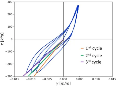
The Figure I-7 shows an example of a real soil sample under a cyclic compressional test (Site KSRH10 of the KIK-net Japanese network Régnier et al., 2016a). The response of this sample clearly shows that the stress-strain (τ/γ) relationship is not linear. In this particular example we can observe that during the traction from the first cycle to the third there is a decrease of the slope. The slope represents the secant shear modulus. We also observe that there is a hysteretic behavior with an unloading path different from the loading path and with the occurrence of permanent displacement under zero stress.
Figure I-7. Hysteric curve for a real sample under a periodic cyclic behavior stress load.
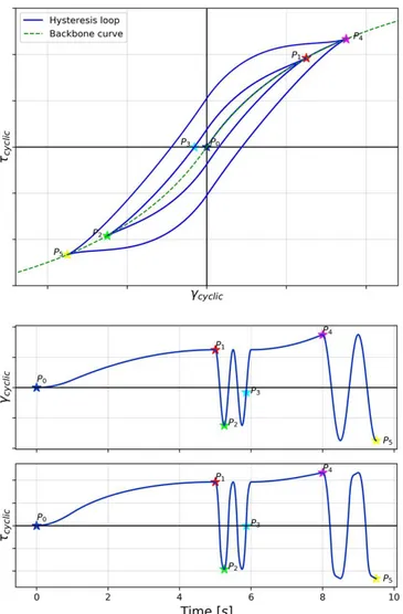
A sketch of the stress-strain relationship of a soil sample that is loaded and unloaded is shown in the Figure I-8 to explain one of the ways to generally analyze the influence of the non-linear soil behavior. First, the sample is loaded slowly from the points P0 to P1. In this case the relationship stress-strain follows a curve that is called backbone curve (Figure I-8, top). The backbone curve for small strains is defined by a constant relationship that is the line Gmax, where Gmax is the slope and it represents the stiffness. After, for higher strains the backbone curve has
a lower slope, representing the loss of stiffness.
From the point P1 to P2 (Figure I-8) the soil sample is unloaded. In this case, the stress-strain
relationship follows a new curve that does not revert to its initial state, zero-zero point (here there is a residual deformation, the material enters the plastic behavior). Under the Masing’s rules (Masing, 1926), the unloading curve is similar to the backbone curve but enlarged by 2. New cycles of loading and unloading are repeated several times from P2 to P3 (Figure I-8). The
loop that is observed after one cycle illustrate the hysteretic behavior of the soil.
The point P3 (Figure I-8) shows a permanent deformation that could not been predicted by a
pure linear method. After from this point (P3) to P4 the soil is load until a higher strain than the previous load. When the loading curve cross the backbone curve, the stress-strains relationship follows the backbone curve (P1 to P4). After a new cyclic load is applied from P4 to P5 defining a
Figure I-8. Sketch of a typical variation of the stress-strain relationship facing cyclic loads (figure based in L. Kramer, 1996, Figure 6.47).
I.2.2 Approximation with G/G
maxcurves and damping curves
To represent the changes of stiffness and in the attenuation due to the non-linear soil behavior, often the modulus reduction curves and damping curves are used (Figure I-9). Those curves show the evolution of these parameters with the strain. Many constitutive models are directly based on these curves, as the hyperbolic model that will be explained on the next section. There are also other more complex models that does not use this kind of curves (e.g. Mellal and Modaressi, 1998).
When using G/Gmax and damping curves, part of the non-linearity process is not taking in
account. For example:
- Under special conditions, as for saturated loose sands, the water that is stored in the soil pores is forced to move during the shaking, creating an increase of the porewater pressure and consequently a variation in the effective stress (the effective stress is the stress that the soil particles really are supporting). During strong shakings, the porewater pressure can increase until the effective stress goes to zero and the soil losses his resistance and start to act like a fluid. This phenomenon is called liquefaction (Mogami and Kubo, 1953; Seed and Idriss, 1971) and this cannot be considered using only damping and the modulus reduction curves.
- Even before liquefaction, the pore water pressure can induce specific behavior like cyclic mobility that cannot be considered by the damping and the modulus reduction curves. - Also, in special situations dynamic solicitations can produce changes in the consolidation of the material. It can create a hardening process on the soil (e.g. Roscoe et al., 1963) that produces plastic strains and it changes the stiffness of the material.
However, the modulus reduction and damping curves are a general and well know way to represent the non-linearity of the soil under cyclic loadings.
Figure I-9. General shape of the shear modulus reduction curves (top) and damping curves (bottom). Gmax represent the shear modulus for small strains. The strain range of the zones is variable for each soil material. The values in this figure are just indicatives, those have a high variability depending of each material.
The modulus reduction curve is normalized by Gmax that is the stiffness of the material at small
strains. This curve and the damping curve can be divided in three parts. The first zone (blue area in Figure I-9) is related with small strains and neither the damping nor the stiffness has a variation. In this zone, the stiffness is the highest in comparison with other zones (Gmax), in the
other hand, the damping in this zone is the lowest (ξmin) and the behavior of the material is
viscoelastic.
In the second zone (green area in Figure I-9) the soils are under moderate strains. The range is approximately between 10-5 to 10-2 (Ishibashi and Zhang, 1993; Seed et al., 1986) although it depends strongly on each material. In this zone the stiffness and the damping present clear changes with respect elastic response, and they are very sensitive to the changes of strains. Finally, the third zone (orange area in Figure I-9) where the soil is under large strains (just as indicative in Figure I-9 this zone starts or γ>10-2, but this threshold variate depending of the soil), the stiffness and the damping are already very low and very high, respectively, in comparison with the values for small strain in the first zone. However, in those zones both parameters, especially the stiffness, starts to converge at some point with the increasing of strain.
I.2.3 Variation of the non-linear behavior due to different parameters
The shear modulus reduction curves (Figure I-9) and the damping curves are characteristic of the material. Those curves have a high variability between materials. Additionally, the non-linear
soil behavior depends also on the soil conditions. For example, the effective stress, the plasticity index, and other factors (Vucetic and Dobry, 1991).
Kokusho, (1980) tested granular materials (sand from Toyoura sand) finding that the modulus reduction and damping curves change with different confinement effective stresses (Figure I-10). For a higher confinement the decay of the stiffness and the damping are lower. It means that the granular soils have a more linear behavior when the effective confinement stress is high.
Figure I-10, Variation of the modulus reduction curve for a similar kind of sand and different confinement stresses. The figure was extracted from (Kokusho, 1980).
Additionally, for granular and sands materials the modulus reduction and damping curves depend of the granulometry of the soil (the distribution of the size particles). Menq, 2003) tested different sandy and gravelly samples, finding a lower elastic zone when the granulometry is less homogenous, (uniformly gradated). It was represented by the relationship between the coefficient of uniformity (Cu) of the soil and the non-linear curves. Even the average size of the particles has not as higher influence as the granulometry.
For the case of the clays, the G/Gmax and damping curves also depends of several factors. The
Figure I-11 shows the variation for this kind of soil in both curves, that was obtained by several studies and summarized in Dobry and Vucetic, 1987). The figures show the influence of the proportions of voids in the soil, measured by the void index (e), and the plastic effect of the clay, measured by the index of plasticity (IP).
In the same study (Dobry and Vucetic, 1987) other factors that influence the modulus reduction and damping curves were analyzed. For stronger confinement stress, the damping curves are reduced (closer to zero) and the G/Gmax curves increase (they become closer to one). It means
that with high confinement stress the clays have a more linear behavior. The geologic age of the material has a similar behavior making more linear the damping and the stiffness. Additionally, since clays usually are commentated materials, the increasing of the cohesion makes also the material more linear.