HAL Id: hal-03127771
https://hal.archives-ouvertes.fr/hal-03127771
Submitted on 2 Feb 2021
HAL is a multi-disciplinary open access
archive for the deposit and dissemination of
sci-entific research documents, whether they are
pub-lished or not. The documents may come from
teaching and research institutions in France or
abroad, or from public or private research centers.
L’archive ouverte pluridisciplinaire HAL, est
destinée au dépôt et à la diffusion de documents
scientifiques de niveau recherche, publiés ou non,
émanant des établissements d’enseignement et de
recherche français ou étrangers, des laboratoires
publics ou privés.
atmospheric inverse applications
P. Kountouris, C. Gerbig, K.-U. Totsche, A. Dolman, A. G. C. A. Meesters,
G. Broquet, F. Maignan, B. Gioli, L. Montagnani, C. Helfter
To cite this version:
P. Kountouris, C. Gerbig, K.-U. Totsche, A. Dolman, A. G. C. A. Meesters, et al.. An objective
prior error quantification for regional atmospheric inverse applications. Biogeosciences, European
Geosciences Union, 2015, 12 (24), pp.7403-7421. �10.5194/bg-12-7403-2015�. �hal-03127771�
www.biogeosciences.net/12/7403/2015/ doi:10.5194/bg-12-7403-2015
© Author(s) 2015. CC Attribution 3.0 License.
An objective prior error quantification for regional
atmospheric inverse applications
P. Kountouris1, C. Gerbig1, K.-U. Totsche2, A. J. Dolman3, A. G. C. A. Meesters3, G. Broquet4, F. Maignan4, B. Gioli5, L. Montagnani6,7, and C. Helfter8
1Max Planck Institute for Biogeochemistry, Jena, Germany
2Institute of Geosciences, Department of Hydrology, Friedrich-Schiller-Universität, Jena, Germany 3VU University Amsterdam, Amsterdam, the Netherlands
4Laboratoire des Sciences du Climat et de l’Environnement, CEA-CNRS-UVSQ, UMR8212, IPSL, Gif-sur-Yvette, France 5Institute of Biometeorology, IBIMET CNR, Florence, Italy
6Faculty of Science and Technology, Free University of Bolzano, Piazza Università 5, 39100 Bolzano, Italy 7Forest Services, Autonomous Province of Bolzano, Via Brennero 6, 39100 Bolzano, Italy
8Centre for Ecology and Hydrology, Edinburgh, UK
Correspondence to: P. Kountouris ([email protected])
Received: 5 May 2015 – Published in Biogeosciences Discuss.: 23 June 2015
Revised: 24 November 2015 – Accepted: 3 December 2015 – Published: 16 December 2015
Abstract. Assigning proper prior uncertainties for inverse modelling of CO2 is of high importance, both to regularise
the otherwise ill-constrained inverse problem and to quanti-tatively characterise the magnitude and structure of the error between prior and “true” flux. We use surface fluxes derived from three biosphere models – VPRM, ORCHIDEE, and 5PM – and compare them against daily averaged fluxes from 53 eddy covariance sites across Europe for the year 2007 and against repeated aircraft flux measurements encompass-ing spatial transects. In addition we create synthetic observa-tions using modelled fluxes instead of the observed ones to explore the potential to infer prior uncertainties from model– model residuals. To ensure the realism of the synthetic data analysis, a random measurement noise was added to the mod-elled tower fluxes which were used as reference. The tempo-ral autocorrelation time for tower model–data residuals was found to be around 30 days for both VPRM and ORCHIDEE but significantly different for the 5PM model with 70 days. This difference is caused by a few sites with large biases between the data and the 5PM model. The spatial correla-tion of the model–data residuals for all models was found to be very short, up to few tens of kilometres but with uncer-tainties up to 100 % of this estimation. Propagating this error structure to annual continental scale yields an uncertainty of 0.06 Gt C and strongly underestimates uncertainties typically
used from atmospheric inversion systems, revealing another potential source of errors. Long spatial e-folding correlation lengths up to several hundreds of kilometres were determined when synthetic data were used. Results from repeated aircraft transects in south-western France are consistent with those obtained from the tower sites in terms of spatial autocorre-lation (35 km on average) while temporal autocorreautocorre-lation is markedly lower (13 days). Our findings suggest that the dif-ferent prior models have a common temporal error structure. Separating the analysis of the statistics for the model data residuals by seasons did not result in any significant differ-ences of the spatial e-folding correlation lengths.
1 Introduction
Atmospheric inversions are widely used to infer surface CO2
fluxes from observed CO2dry mole fractions with a Bayesian
approach (Ciais et al., 2000; Gurney et al., 2002; Lauvaux et al., 2008). In this approach a limited number of obser-vations of atmospheric CO2mixing ratios are used to solve
for generally a much larger number of unknowns, making this an ill-posed problem. By using prior knowledge of the surface–atmosphere exchange fluxes and an associated prior uncertainty, the information retrieved in the inversion from
the observations is spread out in space and time correspond-ing to the spatiotemporal structure of the prior uncertainty. In this way, the solution of the otherwise ill-posed problem is regularised in the sense that the optimisation problem be-comes one with a unique solution. This prior knowledge typ-ically comes from process-oriented or diagnostic biosphere models that simulate the spatiotemporal patterns of terrestrial fluxes, as well as from inventories providing information re-garding anthropogenic fluxes such as energy consumption, transportation, industry, and forest fires.
The Bayesian formulation of the inverse problem is a bal-ance between the a priori and the observational constraints. It is crucial to introduce a suitable prior flux field and assign to it proper uncertainties. When prior information is combined with inappropriate prior uncertainties, this can lead to poorly retrieved fluxes (Wu et al., 2011). Here, we are interested in biosphere–atmosphere exchange fluxes and their uncertain-ties, and we make the usual assumption that the uncertainties in anthropogenic emission fluxes are not strongly affecting the atmospheric observations at the rural sites that are used in the regional inversions of biosphere–atmosphere fluxes.
Typically inversions assume that prior uncertainties have a normal and unbiased distribution and thus can be represented in the form of a covariance matrix. The covariance matrix is a method to weigh our confidence of the prior estimates. The prior error covariance determines to what extent the posterior flux estimates will be constrained by the prior fluxes. Ideally the prior uncertainty should reflect the mismatch between the prior guess and the actual (true) biosphere–atmosphere ex-change fluxes. In this sense it needs to also have the sponding error structure with its spatial and temporal corre-lations.
A number of different assumptions of the error structure have been considered by atmospheric CO2inversion studies.
Coarser-scale inversions often neglect spatial and temporal correlations as the resolution is low enough for the inverse problem to be regularised (Bousquet et al., 1999; Röden-beck et al., 2003a) or assume large spatial correlation lengths (several hundreds of kilometres) over land (Houweling et al., 2004; Rödenbeck et al., 2003b). For the former case, large correlation scales are implicitly assumed since fluxes within a grid cell are fully correlated. For regional-scale inversions, with higher spatial grid resolutions which are often less than 100 km, the spatial correlations are decreased (Chevallier et al., 2012) and the error structure need to be carefully defined. A variety of different assumptions exist. This is because only recently an objective approach to define prior uncertainties based on mismatch between modelled and observed fluxes has been developed (Chevallier et al., 2006, 2012). In some regional studies, the same correlations are used as in large-scale inversions in order to regularise the problem, although the change of resolution could lead to different correlation scales (Schuh et al., 2010). Alternatively, they are defined with a correlation length representing typical synoptic mete-orological systems (Carouge et al., 2010). In other cases, ad
hoc solutions are adopted, where the correlation lengths are assumed to be smaller than in the case of global inversions (Peylin et al., 2005), or derived from climatological and eco-logical considerations (Peters et al., 2007), where correlation lengths only within the same ecosystem types have a value of 2000 km. In addition some studies use a number of differ-ent correlation structures in order to analyse which seems to be the most appropriate one based on cross-validation of the simulated against observed CO2 mole fractions. The
simu-lated mole fractions were derived using the influence func-tions and the inverted fluxes (Lauvaux et al., 2012). Micha-lak et al. (2004) applied a geostatistical approach based on the Bayesian method, in which the prior probability density function is based on an assumed form of the spatial and tem-poral correlation and no prior flux estimates are required. It optimises the prior error covariance parameters, the variance, and the spatial correlation length by maximising the prob-ability density function of the observations with respect to these parameters.
A recent study by Broquet et al. (2013) obtained good agreements between the statistical uncertainties as derived from the inversion system and the actual misfits calculated by comparing the posterior fluxes to local flux measurements at the European and 1-month scales. These good agreements re-lied largely on their definition of the prior uncertainties based on the statistics derived in an objective way from model–data mismatch by Chevallier et al. (2006, 2012). In these stud-ies, modelled daily fluxes from a site-scale configuration of the ORCHIDEE model are compared with flux observations made within the global FLUXNET site network, based on the eddy covariance method (Baldocchi et al., 2001), and a statistical upscaling technique is used to derive estimates of the uncertainties in ORCHIDEE simulations at lower res-olutions. While typical inversion systems have a resolution ranging from tens of kilometres up to several degrees (hun-dreds of kilometres), with the true resolution of the inverse flux estimates being even coarser, the spatial representativity of the flux observations typically covers an area with a ra-dius of around 1 km. Considering also the scarcity of the ob-serving sites in the flux network, the spatial information they bring is limited without methods for up-scaling such as the one applied by Chevallier et al. (2012). Typical approaches to up-scale site level fluxes deploy for example model tree algorithms, a machine learning algorithm which is trained to predict carbon flux estimates based on meteorological data, vegetation properties and types (Jung et al., 2009; Xiao et al., 2008), or neural networks (Papale and Valentini, 2003). Nev-ertheless eddy covariance measurements provide a unique opportunity to infer estimates of the prior uncertainties by examining model–data misfits for spatial and temporal auto-correlation structures.
Hilton et al. (2012) studied also the spatial model– data residual error structure using a geostatistical method. Hilton’s study is focused on the seasonal scale, i.e. investi-gated residual errors of seasonally aggreinvesti-gated fluxes.
How-ever, the state space (variables to be optimized considering also their temporal resolution) of current inversion systems is often at high temporal resolution (daily or even 3-hourly op-timisations). Further, the statistical consistency between the error covariance and the state space is crucial. Thus the er-ror structure at the daily timescale is of interest here and can be used in atmospheric inversions of the same temporal res-olution. Similar to Hilton’s study we select an exponentially decaying model to fit the spatial residual autocorrelation.
In this study, we augment the approach of Chevallier et al. (2006, 2012) to a multi-model–data comparison, investi-gating among others a potential generalisation of the error statistics, suitable to be applied by inversions using different biosphere models as priors. This expectation is derived from the observation that the biosphere models, despite their po-tential differences, typically have much information in com-mon, such as driving meteorological fields, land use maps, or remotely sensed vegetation properties, and sometimes even process descriptions. We evaluate model–model mismatches to (I) investigate intra-model autocorrelation patterns and (II) to explore whether they are consistent with the spatial and temporal e-folding correlation lengths of the model–data mismatch comparisons. Model comparisons have been used in the past to infer the structure of the prior uncertainties. For example, Rödenbeck et al. (2003b) used prior correla-tion lengths based on statistical analyses of the variacorrela-tions within an ensemble of biospheric models. This approach is to a certain degree questionable, as it is unclear how far the ensemble of models actually can be used as representative of differences between modelled and true fluxes. However, if a relationship between model–data and model–model statis-tics can be established for a region with a dense network of flux observations, it could also be used to derive prior error structure for regions with a less dense observational network. Moreover, to improve the knowledge of spatial flux er-ror patterns, we make use of a unique set of aircraft fluxes measured on 2 km spatial windows along intensively sam-pled transects of several tens of kilometres, ideally resolving spatial and temporal variability of ecosystem fluxes across the landscape without the limitation of the flux network with spatial gaps in between measurement locations. Lauvaux et al. (2009) compared results of a regional inversion against measurements of fluxes from aircraft and towers, while this is the first attempt to use aircraft flux measurements to assess spatial and temporal error correlation structures.
This study focuses on the European domain for 2007 (tower data) and 2005 (aircraft data) and uses output from high-resolution biosphere models that have been used for regional inversions. Eddy covariance tower fluxes were de-rived from the FLUXNET ecosystem network (Baldocchi et al., 2001), while aircraft fluxes were acquired within the CarboEurope Regional Experiment (CERES) in southern France. The methods and basic information regarding the models are summaries in Sect. 2. The results from model–
data and model–model comparisons are detailed in Sect. 3. Discussion and conclusions are following in Sect. 4.
2 Data and methods
Appropriate error statistics for the prior error covariance ma-trix are derived from comparing the output of three biosphere models which are used as priors for regional-scale inversions with flux data from the ecosystem network and aircraft. We investigate spatial and temporal autocorrelation structures of the model–data residuals. The temporal autocorrelation is a measure of similarity between residuals at different times but at the same location as a function of the time difference. The spatial autocorrelation refers to the correlation, at a given time, of the model–data residuals at different locations as a function of spatial distance. With this analysis we can formu-late and fit an error model such as an exponentially decaying model, which can be directly used in the mesoscale inversion system to describe the prior error covariance.
2.1 Observations
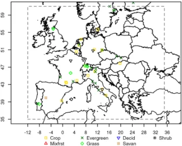
A number of tower sites within the European domain, roughly expanding from −12 to 35◦E and 35 to 61◦N (see also Fig. 1), provide us with direct measurements of CO2
biospheric fluxes using the eddy covariance technique. This technique computes fluxes from the covariance between ver-tical wind velocity and CO2dry mole fraction (Aubinet et al.,
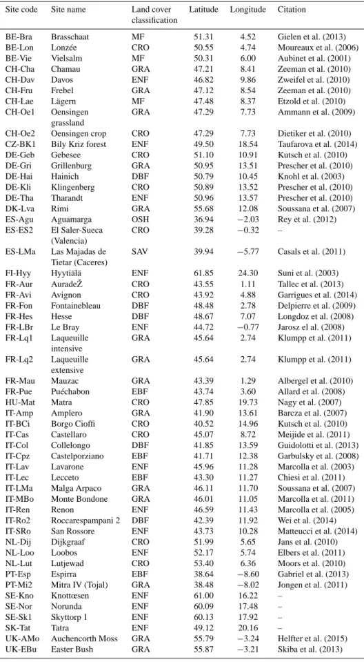
2000). We use Level 3 quality-checked half-hourly observa-tions of net ecosystem exchange fluxes (NEE), downloaded from the European Flux Database (www.europe-fluxdata.eu) and listed by site in Table 1. Each site is categorised into dif-ferent vegetation types (Table 1). A land cover classification is used to label the sites as crop (17 sites), deciduous forest (4), evergreen forest (17), grassland (8), mixed forest (3), sa-vannah (1 site), and shrub land (1). For the current study we focus on observations from these 53 European sites during the year 2007 (Fig. 1).
Additionally, aircraft fluxes are used, obtained with an eddy covariance system installed onboard a SkyArrow ERA aircraft (Gioli et al., 2006). Flights were made in southern France during CERES (CarboEurope Regional Experiment) from 17 May to 22 June 2005. Eddy covariance fluxes were computed on 2 km length spatial windows along transects of 69 km above forest and 78 km above agricultural land, flown 52 and 54 times respectively, covering the daily course. Exact routes are reported in Dolman et al. (2006).
2.2 Biosphere models
We simulate CO2terrestrial fluxes for 2007 with three
differ-ent biosphere models described in the following. The Vege-tation Photosynthesis and Respiration Model (VPRM) (Ma-hadevan et al., 2008), used to produce prior flux fields for inverse studies (Pillai et al., 2012), is a diagnostic model that
Table 1. Eddy covariance sites measuring CO2fluxes that were used in the analysis. The land cover classification used is coded as fol-lows: CRO, DCF, EVG, MF, GRA, OSH, and SAV for crops, deciduous forest, evergreen forest, mixed forest, grass, shrub, and savanna respectively.
Site code Site name Land cover Latitude Longitude Citation classification
BE-Bra Brasschaat MF 51.31 4.52 Gielen et al. (2013) BE-Lon Lonzée CRO 50.55 4.74 Moureaux et al. (2006) BE-Vie Vielsalm MF 50.31 6.00 Aubinet et al. (2001) CH-Cha Chamau GRA 47.21 8.41 Zeeman et al. (2010) CH-Dav Davos ENF 46.82 9.86 Zweifel et al. (2010) CH-Fru Frebel GRA 47.12 8.54 Zeeman et al. (2010) CH-Lae Lägern MF 47.48 8.37 Etzold et al. (2010) CH-Oe1 Oensingen GRA 47.29 7.73 Ammann et al. (2009)
grassland
CH-Oe2 Oensingen crop CRO 47.29 7.73 Dietiker et al. (2010) CZ-BK1 Bily Kriz forest ENF 49.50 18.54 Taufarova et al. (2014) DE-Geb Gebesee CRO 51.10 10.91 Kutsch et al. (2010) DE-Gri Grillenburg GRA 50.95 13.51 Prescher et al. (2010) DE-Hai Hainich DBF 50.79 10.45 Knohl et al. (2003) DE-Kli Klingenberg CRO 50.89 13.52 Prescher et al. (2010) DE-Tha Tharandt ENF 50.96 13.57 Prescher et al. (2010) DK-Lva Rimi GRA 55.68 12.08 Soussana et al. (2007) ES-Agu Aguamarga OSH 36.94 −2.03 Rey et al. (2012) ES-ES2 El Saler-Sueca CRO 39.28 −0.32 –
(Valencia)
ES-LMa Las Majadas de SAV 39.94 −5.77 Casals et al. (2011) Tietar (Caceres)
FI-Hyy Hyytiälä ENF 61.85 24.30 Suni et al. (2003) FR-Aur AuradeŽ CRO 43.55 1.11 Tallec et al. (2013) FR-Avi Avignon CRO 43.92 4.88 Garrigues et al. (2014) FR-Fon Fontainebleau DBF 48.48 2.78 Delpierre et al. (2009) FR-Hes Hesse DBF 48.67 7.07 Longdoz et al. (2008) FR-LBr Le Bray ENF 44.72 −0.77 Jarosz el al. (2008) FR-Lq1 Laqueuille GRA 45.64 2.74 Klumpp et al. (2011)
intensive
FR-Lq2 Laqueuille GRA 45.64 2.74 Klumpp et al. (2011) extensive
FR-Mau Mauzac GRA 43.39 1.29 Albergel et al. (2010) FR-Pue Puéchabon EBF 43.74 3.60 Allard et al. (2008) HU-Mat Matra CRO 47.85 19.73 Nagy et al. (2007) IT-Amp Amplero GRA 41.90 13.61 Barcza et al. (2007) IT-BCi Borgo Cioffi CRO 40.52 14.96 Kutsch et al. (2010) IT-Cas Castellaro CRO 45.07 8.72 Meijide et al. (2011) IT-Col Collelongo DBF 41.85 13.59 Guidolotti et al. (2013) IT-Cpz Castelporziano EBF 41.71 12.38 Garbulsky et al. (2008) IT-Lav Lavarone ENF 45.96 11.28 Marcolla et al. (2003) IT-Lec Lecceto EBF 43.30 11.27 Chiesi et al. (2011) IT-LMa Malga Arpaco GRA 46.11 11.70 Soussana et al. (2007) IT-MBo Monte Bondone GRA 46.01 11.05 Marcolla et al. (2011) IT-Ren Renon ENF 46.59 11.43 Marcolla et al. (2005) IT-Ro2 Roccarespampani 2 DBF 42.39 11.92 Wei et al. (2014) IT-SRo San Rossore ENF 43.73 10.28 Matteucci et al. (2014) NL-Dij Dijkgraaf CRO 51.99 5.65 Jans et al. (2010) NL-Loo Loobos ENF 52.17 5.74 Elbers et al. (2011) NL-Lut Lutjewad CRO 53.40 6.36 Moors et al. (2010) PT-Esp Espirra EBF 38.64 −8.60 Gabriel et al. (2013) PT-Mi2 Mitra IV (Tojal) GRA 38.48 −8.02 Jongen et al. (2011)
SE-Kno Knottœsen ENF 61.00 16.22 –
SE-Nor Norunda ENF 60.09 17.48 –
SE-Sk1 Skyttorp 1 ENF 60.13 17.92 –
SK-Tat Tatra ENF 49.12 20.16 –
UK-AMo Auchencorth Moss GRA 55.79 −3.24 Helfter et al. (2015) UK-EBu Easter Bush GRA 55.87 −3.21 Skiba et al. (2013)
Figure 1. Eddy covariance sites used in the study. The dashed line
delimits the exact domain used to calculate the aggregated fluxes.
uses the enhanced vegetation index (EVI) and land surface water index (LSWI) from MODIS, a vegetation map (Syn-map, Jung et al., 2006) and meteorological data (temperature at 2 m and downward shortwave radiative flux extracted from ECMWF short-term forecast fields at 0.25◦resolution) to de-rive gross biogenic fluxes. VPRM parameters controlling res-piration and photosynthesis for different vegetation types (a total of four parameters per vegetation type) were optimized using eddy covariance data for the year 2005 collected during the CarboEuropeIP project (Pillai et al., 2012). For this study, VPRM fluxes are provided at hourly temporal resolution and at three spatial resolutions of 1, 10 and 50 km (referred to as VPRM1, VPRM10, and VPRM50). The difference between the 1, 10, and 50 km resolution version is the aggregation of MODIS indices to either 1, 10, or 50 km; otherwise the same meteorology and VPRM parameters are used. At 10 km res-olution VPRM uses a tiled approach, with fractional cover-age for the different vegetation types and vegetation-type-specific values for MODIS indices. For the comparison with the aircraft data VPRM produced fluxes for 2005 at 10 km spatial resolution.
The Organising Carbon and Hydrology In Dynamic Ecosystems (ORCHIDEE) model (Krinner et al., 2005) is a process-based site scale to global land surface model that simulates the water and carbon cycle using meteorological forcing (temperature, precipitation, humidity, wind, radia-tion, pressure). The water balance is solved at a half-hourly time step while the main carbon processes (computation of a prognostic leaf area index (LAI), allocation, respiration, turnover) are called on a daily basis. It uses a tiled approach, with fractional coverage for 13 plant functional types (PFTs). It has been extensively used as prior information in regional-and global-scale inversions (Piao et al., 2009; Broquet et al., 2013). For the present simulation, we use a global
configura-tion of the version 1.9.6 of ORCHIDEE, where no parameter has been optimized against eddy covariance data. The model is forced with 0.5◦ WFDEI meteorological fields (Weedon
et al., 2014). The PFT map is derived from an Olson land cover map (Olson, 1994) based on AVHRR remote sensing data (Eidenshink and Faundeen, 1994). The fluxes are diag-nosed at 3-hourly temporal resolution and at 0.5◦horizontal resolution.
The “5 parameter model” (5PM) (Groenendijk et al., 2011), also used in atmospheric inversions (Tolk et al., 2011; Meesters et al., 2012), is a physiological model describing transpiration, photosynthesis, and respiration. It uses MODIS LAI at 10 km resolution, meteorological data (temperature, moisture, and downward shortwave radiative flux, presently from ECMWF at 0.25◦resolution), and differentiates PFTs for different vegetation types and climate regions. 5PM fluxes are at hourly temporal resolution. The optimisation has been done with eddy covariance (EC) data from FLUXNET as described (except for heterotrophic respiration) in Groe-nendijk et al. (2011). Regarding the heterotrophic respiration, an ad hoc optimisation using FLUXNET EC data from 2007 was performed since no previous optimisation was available. Modelled fluxes for all above mentioned sites have been provided by the different models by extracting the fluxes from the grid cells which encompass the EC station location using vegetation-type-specific simulated fluxes, i.e. using the vegetation type within the respective grid cell for which the eddy covariance site is assumed representative. For most of the sites the same vegetation type was used for model ex-traction as long as this vegetation type is represented within the grid cell. As VPRM uses a tile approach, for two cases (IT-Amp and IT-MBo) the represented vegetation type (crop) differs from the actual one (grass). For these cases, the fluxes corresponding to crop were extracted. Fluxes were aggre-gated to daily fluxes in the following way: first, fluxes from VPRM and 5PM as well as the observed fluxes were tem-porally aggregated to match with the ORCHIDEE 3-hourly resolution; in a second step we created gaps in the modelled fluxes where no observations were available; the last step ag-gregated to daily resolution on the premise that (a) the gaps covered less than 50 % of the day and (b) the number of gaps (number of individual 3-hourly missing values) during day and during night were similar (not different by more than a factor two) to avoid biasing.
Spatial and temporal correlation structures and the stan-dard deviation of flux residuals (model–observations) were examined for daily fluxes over the year 2007. Simulated fluxes from the different models are at different spatial resolution, which makes comparisons difficult to interpret. For the model–data residual analysis, the models VPRM1, VPRM10, ORCHIDEE, and 5PM were used. We note that VPRM1 with 1 km resolution is considered compatible when comparing with local measurements. For the model–model analysis we use VPRM50 at 50 km resolution when com-paring with ORCHIDEE fluxes as both models share the
same resolution. VPRM10 is considered also appropriate for comparisons with 5PM model as they both share the same resolution (MODIS radiation resolution of 1 km aggregated to 10 km and meteorological resolution at 0.25◦). Further, we compare VPRM50 with 5PM to investigate whether the different spatial resolution influences the correlation scale as a measure of how trustworthy the derived scales from ORCHIDEE–5PM comparisons might be.
For the aircraft analysis, only the VPRM was used since it is the only model with spatial resolution (10 km) comparable with aircraft flux footprint and capable of resolving spatial variability in relatively short flight distances. Aircraft NEE data, natively at 2 km resolution along the track, have been aggregated into 10 km segments to maximise the overlap with the VPRM grid, obtaining six grid points in forest tran-sects and eight in agricultural land trantran-sects. Footprint areas of aircraft fluxes were computed with the analytical model of Hsieh et al. (2000), yielding an average footprint width containing 90 % of the flux of 3.9 km. Averaging also over the different wind directions (perpendicular or parallel to the flight direction) and taking into account the 10 km length of the segments, the area that the aircraft flux data corresponds to, is around 23.5 km ± 12 km2. VPRM fluxes at each aircraft grid cell were extracted and then linearly interpolated to the time of each flux observation.
2.3 Analysis of model–observation differences
Observed and modelled fluxes are represented as the sum of the measured or simulated values and an error term respec-tively. When we compare modelled to observed data this er-ror term is a combination of model (the prior uncertainty we are interested in) and observation error. Separating the obser-vation error from the model error in the statistical analysis of the model–observation mismatch is not possible; there-fore e-folding correlation length estimations do include the observation error term. Nevertheless, later in the analysis of model–model differences we assess the impact of the obser-vation error on estimated e-folding correlation lengths.
The tower temporal autocorrelation is computed between the time series of model–observations differences xl,iat site
l and the same series lagged by a time unit k (Eq. 1), where
x is the overall mean and N the number of observations:
rl(k) = N −k P i=1 (xl,i−xl) · (xl,i+k−xl) N P i=1 (xl,i−xl)2 . (1)
In order to reduce boundary effects in the computation of the autocorrelation at lag times around 1 year, the 1-year flux time series data (model and observations) for each site was replicated four times. This follows the approach of Chevallier et al. (2012), where sites with at least 3 consecutive years of measurements have been used.
In the current analysis we introduce the all-site temporal autocorrelation by simultaneously computing the autocorre-lation for all the observation sites, where M is the number of the sites: r(k) = M P l=1 N −k P i=1 (xl,i−xl) · (xl,i+k−xl) M P l=1 N P i=1 (xl,i−xl)2 . (2)
Temporal correlation scales τ were derived by fitting an ex-ponentially decaying model:
r = (1 − α) · e−τt. (3)
Here t is the time lag. For the exponential fit, lags up to 180 days were used (thus the increase in correlations for lag times larger than 10 months is excluded). At 0 lag time the correlogram has a value of 1 (fully correlated); however for even small lag times this drops to values smaller than 1, also known as the nugget effect. The nugget effect is driven by measurement errors and variations at distances (spatial or temporal) smaller than the sampling interval. For this we in-clude the nugget effect variable α.
The aircraft temporal autocorrelation was similarly com-puted according to Eq. (1) using VPRM, and the same expo-nentially decaying model (Eq. 3) was used to fit the individ-ual flight flux data. The temporal interval was limited at 36 days by the experiment duration.
For the spatial analysis the correlation between model– observation residuals at two different locations (i.e sites or aircraft grid points) separated by a specific distance was com-puted in a way similar to the temporal correlation and in-volved all possible pairs of sites and aircraft grid points. Ad-ditional data treatment for the spatial analysis was applied to reduce the impact of tower data gaps, as it is possible that the time series for two sites might have missing data at different times. Thus in order to have more robust results, we also ex-amined spatial structures by setting a minimum threshold of 150 days of overlapping observations within each site pair. Furthermore spatial correlation was investigated for seasonal dependence, where seasons are defined as summer (JJA), au-tumn (SON), winter (DJF for the same year), and spring (MAM). In those cases a different threshold of 20 days of overlapping observations was applied. We note that we do not intend to investigate the errors at the seasonal scale but rather to study whether different seasons trigger different er-ror correlation structures.
To estimate the spatial correlation scales, the pairwise cor-relations were grouped into bins of 100 km distance for tow-ers and 10 km for aircraft data respectively (dist). Following the median for each bin was calculated, and a model similar to Eq. (3) was fitted but omitting the nugget effect variable:
The nugget effect could not be constrained simultaneously with the spatial correlation scale d given the relatively coarse distance groups, the fast drop in the median correlation from 1 at 0 distance to small values for the first distance bin com-bined with somewhat variations at larger distances. Note that this difference between the spatial and the temporal correla-tion becomes obvious in the results Sect. 3.
Confidence intervals for the estimated model parame-ters were computed based on the profile likelihood (Venzon and Moolgavkar, 1988) as implemented within the “confint” function from MASS package inside the R statistical lan-guage.
As aircraft fluxes cannot obviously be measured at the same time at different locations, given the relatively short flight duration (about 1 h) we treated aircraft flux transect as instantaneous “snapshots” of the flux spatial pattern across a landscape, neglecting temporal variability that may have oc-curred during flight.
2.4 Analysis of model–model differences
We evaluate both model–data flux residuals and model– model differences in a sense of pairwise model comparisons, in order to assess whether model–model differences can be used as proxy for the prior uncertainty, assuming that mod-els have independent prior errors. In order to minimise po-tential influence of the different spatial resolution between the models on the estimated correlation lengths, we com-pare pairs that have comparable spatial resolution. Such cases are VPRM50–ORCHIDEE and VPRM10–5PM. We choose VPRM10 as more representative to compare against 5PM as 5PM fluxes have also a resolution of 10 km (the main driver, MODIS radiation has the same resolution of 10 km for both models). Similar to the model–observation analysis, the sta-tistical analysis gives a combined effect of both model errors. We assess the impact in the error structure between model– observation and model–model comparisons caused by the observation error by adding a random measurement error to each model–model comparison. This error has the same char-acteristics as the observation error which is typically asso-ciated with eddy covariance observations; the error charac-teristics were derived from the paired observation approach (Richardson et al., 2008). Specifically, we implement the flux observation error as a random process (white noise) with a double-exponential probability density function. This can be achieved by selecting a random variable u drawn from the uniform distribution in the interval (−1/2, 1/2) and then ap-plying Eq. (5) to get a Laplace distribution (also referred to as the double exponential):
x = µ −√σ
2
·sgn(u) · ln (1 − 2 · |u|) . (5)
Here µ = 0 and σ is the standard deviation of the double exponential. We compute the σ according to Richardson et
al. (2006) as
σ = α1+α2· |F | , (6)
where F is the flux and α1, α2are scalars specific to the
dif-ferent vegetation classes. Lasslop et al. (2008) found that the autocorrelation of the half-hourly random errors is below 0.7 for a lag of 30 min and falls off rapidly for longer lag times. Thus we assume the standard deviation for hourly random errors to be comparable with the half-hourly errors. Hourly random errors specific for each reference model are gener-ated for each site individually. With ORCHIDEE as refer-ence with fluxes at hourly resolution, a new ensemble of 3-hourly random noise was generated with σ for the 3-3-hourly errors modified (divided by the square root of 3 to be co-herent with the hourly σ ). As both modelled and observed fluxes share the same gaps, the random errors were aggre-gated to daily resolution, with gaps such to match those of observed fluxes. Finally the daily random errors were added to the modelled fluxes.
3 Results
3.1 Model–data comparison for tower and aircraft fluxes
Observed daily averaged NEE fluxes, for all ground sites and the full time series, yield a standard deviation of 3.01 µmol m−2s−1, while the modelled fluxes were found to be less spatially varying and with a standard deviation of 2.84, 2.80, 2.53, and 2.64 µmol m−2s−1 for VPRM10,
VPRM1, ORCHIDEE, and 5PM respectively.
The residual distribution of the models defined as the dif-ference between simulated and observed daily flux averages for the full year 2007 was found to have a standard devia-tion of 2.47, 2.49, 2.7, and 2.25 µmol m−2s−1for VPRM10, VPRM1, ORCHIDEE, and 5PM respectively. Those values are only slightly smaller than the standard deviations of the observed or modelled fluxes themselves. This fact is in line with the generally low fraction of explained variance with
r-square values of 0.31, 0.27, 0.12, and 0.25 for VPRM10, VPRM1, ORCHIDEE, and 5PM respectively. When using site-specific correlations (correlations computed for each site, then averaged over all sites), the average fraction of explained variance increases to 0.38, 0.36, 0.35, and 0.42 for VPRM10, VPRM1, ORCHIDEE, and 5PM respectively. Note that for deseasonalised time series (using a second-order harmonic, not shown) the same picture emerges with increased averaged site-specific correlation compared to cor-relations using all sites. This indicates better performance for the models to simulate temporal changes (not only sea-sonal, but also synoptic) at the site level. Further, the differ-ences between site-specific and overall r-square values indi-cate limitation of the models to reproduce observed spatial (site to site) differences. Figure 2 shows the correlation
be-Figure 2. Box and whisker plot for site-specific correlation
coef-ficients between modelled and observed daily fluxes as a function of the vegetation type. The numbers beneath the x axis indicate the number of sites involved. The bottom and the top of the box denote the first and the third quartiles. The band inside the box indicates the central 50 % and the line within is the median. Upper and lower line edges denote the maximum and the minimum values excluding outliers. Outliers are shown as circles.
tween modelled and observed daily fluxes as a function of the vegetation type characterising each site. All models ex-hibit a significant scatter of the correlation ranging from 0.9 for some sites to 0 or even negative correlation for some crop sites, with the highest correlation coefficients for deciduous and mixed forest.
The distribution is biased by −0.07, 0.26, 0.92, and 0.25 µmol m−2s−1for VPRM10, VPRM1, ORCHIDEE, and 5PM respectively. Figure 3 shows the distribution of bias (de-fined as modelled–observed fluxes) for different vegetation types. Bias and standard deviation seem to depend on the vegetation type for all models, without a clear general pat-tern.
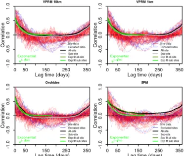
The temporal autocorrelation was calculated for model– data residuals for each of the flux sites (“site data” in Fig. 4), but also for the full data set (“all-site” in Fig. 4). The all-site temporal autocorrelation structure of the residuals appears to have the same pattern for all models. It decays smoothly for time lags up to 3 months and then remains constant near to 0 or to some small negative values. The temporal autocor-relation increases again for time lags > 10 months, which is caused by the seasonal cycle. These temporal autocorrelation results agree with the findings of Chevallier et al. (2012).
The exponentially decaying model in Eq. (3) was used to fit the data. At 0 separation time (t = 0) the correlogram value is 1. However the correlogram exhibits a nugget effect (values ranging from 0.31 to 0.48 for the different models) as a consequence of an uncorrelated part of the error. For the
Figure 3. Box and whisker plot for the annual site-specific biases
of the models differentiated by vegetation type. Units at y axis are in µmol m−2s−1(for conversion to gC m−2yr−1reported values in y axis should be multiplied by 378 7694).
Figure 4. Temporal lagged autocorrelation from model–data daily
averaged NEE residuals for all models. Thin red lines correspond to different sites, while the blue thin lines reveal the sites with a bias larger than ±2.5 µmol m−2s−1. The thick black line shows the all-site autocorrelation, and the thick grey line indicates the all-site autocorrelation but for a subset that excludes sites with large model– data bias (“sub-site”). The dark green line is the all-site exponential fit, and the light green line shows the all-site autocorrelation exclud-ing the sites with large bias. The exponential fits use lag times up to 180 days.
current analyses we fit the exponential model with an initial correlation different from 1. The fit has a root mean square error ranging from 0.036 to 0.059 for the different biosphere models. The normalised root mean square error (RMSE) (i.e.
RMSE divided by the range of the autocorrelation) results in values ranging from 0.061 to 0.092, indicating relative errors in the fit of less than 10 %. The e-folding time (defined as the lag required for the correlation to decrease by a factor of e (63 % of its initial value) ranged between 26 and 70 days for the different models (see Table 2). Specifically, for VPRM10 and VPRM1 the e-folding time is 32 and 33 days respec-tively (30–34 days within 95 % confidence interval for both). Confidence intervals for the e-folding time were calculated by computing the confidence intervals of the parameter in the fitted model. For ORCHIDEE best fit was 26 days (23– 28 days within 95 % confidence interval). In contrast, 5PM yields a significantly longer correlation time between 65 and 75 days (95 % confidence interval) with the best fit being 70 days.
For a number of sites a large model–data bias was found. In order to assess how the result depends on individual sites where model–data residuals are more strongly biased the analysis was repeated under exclusion of sites with an annual mean of model–data flux residuals larger than 2.5 µmol m−2s−1. This threshold value is roughly half of the most deviant bias. In total nine sites (CH-Lae, ES-ES2, FR-Pue, IT-Amp, IT-Cpz, IT-Lav, IT-Lec, IT-Ro2, PT-Esp) across all model–data residuals were excluded. From these sites, CH-Lae appears to have serious problems related to the steep terrain, where the basic assumptions made for eddy covariance flux measurements are not applicable (Göckede et al., 2008). The rest of the sites are located in the Mediter-ranean region and suffer from summer drought according to the Köppen–Geiger climate classification map (Kottek et al., 2006); in those cases a large model–data bias is expected as existing models tend to have difficulties estimating carbon fluxes for drought-prone periods (Keenan et al., 2009). The model–data bias at those sites does not necessarily exceed the abovementioned threshold of 2.5 µmol m−2s−1 simulta-neously for each individual model, but a larger bias than the average was detected. After exclusion of those sites the tem-poral correlation times were found to be between 33 and 35 days within 95 % confidence interval for 5PM with the best-fit value being 34 days. The rest of the models had temporal e-folding times of 27, 29, and 24 days (first row of Table 2), while the all-site correlation remains positive for lags < 76, < 79, and < 66 days for VPRM10, VPRM1, and ORCHIDEE respectively. Some weak negative correlations exist, with a minimum value of −0.06, −0.02, −0.09, and −0.005 for VPRM10, VPRM1, ORCHIDEE, and 5PM respectively.
The temporal correlation of differences between VPRM10 and aircraft flux measurements could be computed for time intervals up to 36 days (Fig. 5) corresponding to the duration of the campaign. The correlation shows an exponential de-crease and levels off after about 25 days with an e-folding correlation time of 13 days (range of 10–16 days within the 95 % confidence interval). Whilst the general behaviour is consistent with results obtained for VPRM–observation residuals for flux sites, the correlation time is 2 times smaller.
Figure 5. Temporal autocorrelation for VPRM10–aircraft NEE
residuals. Black dots represent individual flux transects pairs sam-pled at different times as function of time separation. Black circles represent daily-scale binned data.
Regarding spatial error correlations, results for all models show a dependence on the distance between pairs of sites. The median correlation drops within very short distances (Fig. 6). Fitting the simple exponentially decaying model (Eq. 4) to the correlation as a function of distance we find an e-folding correlation length d of 40, 37, 32, and 31 km with a RMSE of 0.14, 0.09, 0.05, and 0.07 for VPRM10, VPRM1, ORCHIDEE, and 5PM respectively. The normalised RMSE is found to have values ranging from 0.05 to 0.084 indicat-ing relative errors of the fit less than 9 %. Spatial correlation scales are also computed for a number of different data selec-tions (cases) in addition to the standard case shown in Fig. 6 (case S): using only pairs with at least 150 overlapping days of non-missing data (case S∗), using only pairs with identi-cal PFT (case I), using only pairs with different PFT (case D), and using only pairs with at least 150 overlapping days for the D and I cases (cases D∗, I∗). The results for these cases are summarised in Fig. 7. Also 95 % confidence inter-vals were computed, and the spread spatial correlation was found to be markedly more critical than for the time correla-tions. Note that for some cases the 2.5 percentile (the lower bound of the confidence interval) hit the lower bound for cor-relation lengths (0 km). The e-folding corcor-relation lengths are similar for each of the models: this also means that no de-pendence on the spatial resolution was detectable. Further, we examined also the spatial autocorrelation from VPRM50– data residuals with no significant difference compared to pre-vious results.
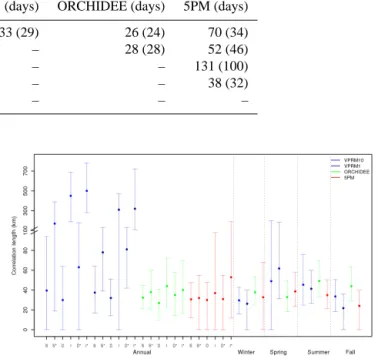
Table 2. Annual temporal autocorrelation times in days, from model–data and model–model residuals. The number within the brackets shows
the correlation times when excluding sites with large model–data bias from the analysis.
Reference VPRM10 (days) VPRM1 (days) ORCHIDEE (days) 5PM (days)
OBSERVATION 32 (27) 33 (29) 26 (24) 70 (34)
VPRM50 – – 28 (28) 52 (46)
VPRM10 – – – 131 (100)
ORCHIDEE – – – 38 (32)
5PM – – – –
Figure 6. Distance correlogram for the daily net ecosystem
ex-change (NEE) residuals using all sites. Black dots represent the dif-ferent site pairs; the blue line represents the median value of the points per 100 km bin and the green an exponential fit. Results are shown for residuals of VPRM at a resolution of 10 (top left) and 1 km (top right), ORCHIDEE (bottom left), 5PM (bottom right).
Interestingly, if we restrict the analysis to pairs with at least 150 overlapping days between site pairs, larger cor-relation scales are found (case S∗ in Fig. 7). Considering only pairs with different PFT (case D), consistently, all e-folding correlation lengths are found to be smaller compared to the standard case (S). This is expected to a certain de-gree, as model errors should be more strongly correlated be-tween sites with similar PFTs than bebe-tween sites with differ-ent PFTs. By considering only pairs within the same vege-tation type (case I) we observe a significant increase of the e-folding correlation length relative to case S for VPRM at 10 and 1 km resolution to values of 432 km and 305 km re-spectively. The ORCHIDEE and 5PM models show some (although not significant) increase in e-folding correlation length. Restricting again the analysis to pairs with at least 150 overlapping days for the D and I cases (D∗, I∗) we ob-serve an increase of the e-folding correlation lengths that is, however, significant only for VPRM at 10 and 1 km.
Figure 7. Annual and seasonal e-folding correlation length of the
daily averaged model–data NEE residuals for VPRM at 10 and 1 km resolution, ORCHIDEE and 5PM. S refers to the standard case where all pairs were used, D refers to the case where only pairs with different vegetation types were used, I denotes the case in which only pairs with identical vegetation type were considered, and∗ de-notes that in addition 150 days of common non-missing data are required for each pair of sites. The dot represents the best-fit value when fitting the exponential model. The upper and the lower edge of the error bars show the 2.5 and 97.5 percentiles of the length value. Note the scale change in the y axis at 100 km.
Seasonal dependence of the e-folding correlation lengths for at least 20 overlapping days per season and for all-site pairs is also shown in Fig. 7. VPRM showed somewhat longer correlation lengths during spring and summer, OR-CHIDEE had the largest lengths occurring during summer and autumn, and 5PM e-folding correlation lengths show slightly enhanced values during spring and summer. How-ever, none of these seasonal differences are significant with respect to the 95 % confidence interval.
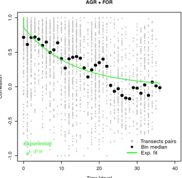
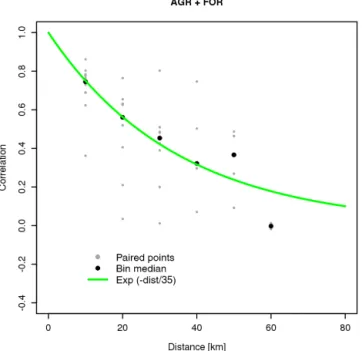
The spatial error correlation between VPRM10 model and aircraft fluxes measured during May–June along continuous transects at forest and agriculture land use (Fig. 8) shows an exponential decay up to the maximum distance that was en-compassed during flights (i.e. 70 km). Of note is that only two measurements were available at 60 km distance and none for larger distances making it difficult to identify where the asymptote lies. Nevertheless, fitting the decay model (Eq. 4) leads to d = 35 km (26–46 km within the 95 % confidence interval), which is in good agreement with the spatial
corre-Figure 8. Distance correlogram between VPRM10 and aircraft
NEE measurements. Black dots represents the different aircraft grid points pairs; black circles represent 10 km scale binned data.
lation scale derived for VPRM10 using flux sites during both spring and summer (Fig. 7).
3.2 Model–model comparison
We investigate the model–model error structure of NEE es-timates by replacing the observed fluxes which were used as reference, with simulated fluxes from all the biosphere models. Note that for consistency with the model–data anal-ysis, the simulated fluxes contained the same gaps as the observed flux time series. The e-folding correlation time is found to be slightly larger compared to the model–data cor-relation times, for most of the cases. An exception is the 5PM–VPRM10 pair which produced remarkably larger cor-relation time (Table 2). Specifically, VPRM50–ORCHIDEE and VPRM10–5PM residuals show correlation times of 28 days (range between 24 and 32 days within 95 % confidence interval) and 131 (range between 128 and 137 days within 95 % confidence interval) respectively. Significantly differ-ent e-folding correlation times are found for VPRM50–5PM compared to VPRM10–5PM with correlation times of 52 days (range between 49 and 56 days within 95 % confidence interval). Repeating the analysis excluding sites with resid-ual bias larger than 2.5 µmol m−2s−1, correlation times of 28 and 100 days for VPRM50–ORCHIDEE and VPRM10– 5PM are found respectively. If we use the ORCHIDEE–5PM pair, the e-folding correlation time is 38 days (range between 35 and 41 days within 95 % confidence interval).
Although the e-folding correlation times show only mi-nor differences compared to the model–data residuals, this
Figure 9. Annual and seasonal e-folding correlation length for an
ensemble of daily averaged NEE differences between two models without (filled circle) and with random measurement errors added to the modelled fluxes used as reference (crosses). The symbols rep-resents the best-fit value when fitting the exponential model, and the upper and lower edge of the error bars show the 2.5 and 97.5 per-centiles of the correlation length. The first acronym at the legend represents the model used as reference and the second the model which was compared with. Note that for the VPRM10/VPRM1 case during spring (with and without random error), the 97.5 percentile of the length value exceeds the y axis and has a value of 1073, 1626 km respectively.
is not the case for the spatial correlation lengths (Fig. 9). The standard case (S) was applied for the annual analysis, with no minimum number of days with overlapping non-missing data for each site within the pairs. Taking VPRM50 as reference, much larger e-folding correlation lengths of 371 km with a range of 286–462 km within 95 % confi-dence interval yielded for VPRM50–ORCHIDEE compar-isons, and 1066 km for VPRM50–5PM were found. How-ever, VPRM10–5PM analysis, which is also considered appropriate in terms of the spatial resolution compatibil-ity contrary to the VPRM50–5PM pair, is in good agree-ment with VPRM50–ORCHIDEE spatial scale (230–440 km range within 95 % confidence interval with the best fit be-ing 335 km). With ORCHIDEE as reference, the e-foldbe-ing correlation length for the ORCHIDEE–5PM comparison is 276 km with a range of 183–360 km within 95 % confidence interval. However the later correlation length might be af-fected by the different spatial resolution as the difference be-tween VPRM10 and VPRM50 against 5PM suggests. Sea-sonal e-folding correlation lengths, using a minimum of 20 days overlap in the site-pairs per season (Fig. 9), are also sig-nificantly larger compared with those from the model–data analysis.
When we add the random measurement error to the mod-elled fluxes used as reference (crosses in Fig. 9), we ob-serve only slight changes in the annual e-folding correlation lengths, without a clear pattern. The correlation lengths show a random increase or decrease but limited up to 6 %.
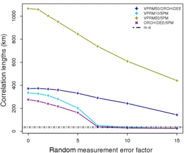
Interest-Figure 10. Annual e-folding correlation lengths as a function of
the factor used for scaling the random measurement error, for all model–model combinations. The black dot-dash lines reveal the range of the spatial correlation lengths generated from the model– data comparisons.
ingly, the seasonal e-folding correlation lengths for most of the cases show a more clear decrease. For example, the cor-relation length of the VPRM10–5PM residuals during win-ter decreases by 22 % or even more for spring season. De-spite this decrease, the e-folding seasonal correlation lengths remain significantly larger in comparison to those from the model–data analysis. Overall, all models when used as ref-erence show the same behaviour with large e-folding cor-relation lengths that mostly decrease slightly when the ran-dom measurement error is included. Although the ranran-dom measurement error was added as “missing part” to the mod-elled fluxes to better mimic actual flux observations, it did not lead to correlation lengths similar to those from the model– data residual analysis. To investigate whether a larger random measurement error could cause spatial correlation scales in model–model differences, we repeated the analysis with ar-tificially increased random measurement error (multiplying with a factor between 1 and 15). Only for very large random measurement errors did the model–model e-folding correla-tion lengths start coinciding with those of the model–data residuals (Fig. 10).
4 Discussion and conclusions
We analysed the error structure of a priori NEE uncertainties derived from a multi-model–data comparison by comparing fluxes simulated by three different vegetation models to daily averages of observed fluxes from 53 sites across Europe, cat-egorised into seven land cover classes. The different models showed comparable performance with respect to
reproduc-ing the observed fluxes; we found mostly insignificant differ-ences in the mean of the residuals (bias) and in the variance. Site-specific correlations between simulated and observed fluxes are significantly higher than overall correlations for all models, which suggest that the models struggle with repro-ducing observed spatial flux differences between sites. Fur-thermore, the site-specific correlations reveal a large spread even within the same vegetation class, especially for crops (Fig. 2). This is likely due to the fact that none of the mod-els uses a specific crop model that differentiates between the different crop types and their phenology. The models using remotely sensed vegetation indices (VPRM and 5PM) better capture the phenology; ORCHIDEE is the only model that differentiates between C3and C4plants but shows the largest
spread in correlation for the crop. Differences in correlations between the different vegetation types were identified for all the biosphere models; however it must be noted that the num-ber of sites per vegetation type is less than 10 except for crop and evergreen forests.
Model–data flux residual correlations were investigated to give insights regarding prior error temporal scales which can be adopted by atmospheric inversion systems. Whilst fluxes from ORCHIDEE model are at much coarser resolution com-pared to the representative area from the flux measurements, VPRM1 fluxes (1 km resolution and only the meteorology at 25 km) are considered appropriate for the comparisons. Despite the scale mismatch, results are in good agreement across all model–data pairs.
Exponentially decaying correlation models are a dominant technique among atmospheric inverse studies to represent temporal and spatial flux autocorrelations (Rödenbeck et al., 2009; Broquet et al., 2011, 2013). However, regarding the temporal error structure we need to note the weakness of this model to capture the slightly negative values at 2–10 months lags and, more importantly, the increase in correlations for lag times larger than about 10 months. Error correlations were parameterized differently by Chevalier et al. (2012) where the prior error was investigated without implement-ing it to atmospheric inversions. Polynomial and hyperbolic equations were used to fit temporal and spatial correlations respectively. Nevertheless, we use here e-folding lengths not only for their simplicity in describing the temporal correla-tion structure with a single number but also because this er-ror model ensures a positive definite covariance matrix (as required for a covariance). This is crucial for atmospheric inversions as otherwise negative, spatially and temporally in-tegrated uncertainties may be introduced. In addition it can keep the computational costs low, because the hyperbolic equation has significant contributions from larger distances: for the case of the VPRM1 model, at 200 km distance the correlation according to Chevallier et al., hyperbolic equa-tion is 0.16 compared to 0.004 for the exponential model. As a consequence, more non-zero elements are introduced to the covariance matrix, which increases computational costs in the inversion systems. Using the same hyperbolic equation
for the spatial correlation, d values of 73, 39, 12, and 20 km were found with a RMSE of 0.11, 0.07, 0.05, and 0.07 for VPRM10, VPRM1, ORCHIDEE, and 5PM respectively. A similar RMSE was found when using the exponential (0.14, 0.09, 0.05, and 0.07), indicating similar performance of both approaches with respect to fitting the spatial correlation.
Autocorrelation times were found to be in line with find-ings of Chevallier et al. (2012). The model–data residuals were found to have an e-folding time of 32 and 26 days for VPRM and ORCHIDEE respectively and 70 days for 5PM. This significant difference appears to have a strong depen-dence on the set of sites used in the analysis. Excluding nine sites with large residual bias, the autocorrelation time from the 5PM–data residuals drastically decreased and became co-herent with the times of the other biosphere models. The all-models and all-site autocorrelation time was found to be 39 days, which reduces to 30 days (28–31 days within 95 % con-fidence interval), when excluding the sites with large residual bias, coherent with the single model times. From the model– model residual correlation analysis, the correlation time ap-pear to be consistent with the above-mentioned results and lies between 28 and 46 days for most of the ensemble mem-bers. However model–model pairs consisting of the VPRM and 5PM models produced larger times up to 131 days; omit-ting sites with large residual biases this is reduced to 100 days (99–105 days within 95 % confidence interval). This finding could be attributed to the fact that despite the conceptual dif-ference between those models, they do have some common properties. Both models were optimized against eddy covari-ance data although for different years (2005 and 2007 re-spectively), while no eddy covariance data were used for the optimisation of ORCHIDEE. In addition, VPRM and 5PM both use data acquired from MODIS, although they estimate photosynthetic fluxes by using different indices of reflectance data. Summarising the temporal correlation structure, it ap-pears reasonable to (a) use the same error correlation in at-mospheric inversions regardless of which biospheric model is used prior or (b) use an autocorrelation length of around 30 days.
Only weak spatial correlations for model–data residuals were found, comparable to those identified by Chevallier et al. (2012) that were limited to short lengths up to 40 km with-out any significant difference between the biospheric models (31–40 km). Hilton et al. (2012) estimated spatial correlation lengths of around 400 km. However, we note that significant differences exist between this study and Hilton et al. (2012) regarding the methods that were used and the landscape het-erogeneity of the domain of interest. With respect to the first aspect the time resolution is much coarser (seasonal aver-aged flux residuals) compared to the daily averaver-aged residuals used here. Furthermore spatial bins of 300 km were used for the autocorrelation analysis, which is far larger than the ap-proximate bin width of 100 km that were used in our study. Regarding the second aspect North America has a more ho-mogenous landscape compared to the European domain. The
scales for each ecosystem type (e.g. forests, agricultural land) are drastically larger than those in Europe as can be seen from MODIS retrievals (Friedl et al., 2002).
Although the estimated spatial scales are shorter than the spatial resolution that we are solving for (100 km bins), the autocorrelation analysis of aircraft measurements made dur-ing CERES supports the short-scale correlations. These mea-surements have the advantage of providing continuous spa-tial flux transects along specific tracks that were sampled rou-tinely (in this case over period of 36 days at various times of the day), thus also resolving flux spatial variability at small scales, where pairs of eddy covariance sites may not be suffi-ciently close. However, aircraft surveys are necessarily spo-radic in time. Of note is that the eddy covariance observa-tion error has no significant impact on the error structure, as the addition of an observation error to the analysis of model–model differences had only minor influence on the error structure. We note that the current analysis focuses to daily timescale and therefore the error statistics with respect to the estimated spatial and temporal e-folding correlation lengths are valid for such scales.
Model–data residual e-folding correlation lengths show a clear difference between the cases where pairs only with dif-ferent (D) or identical (I) PFT were considered, with the lat-ter resulting in longer correlation lengths but only identified for the VPRM model at both resolutions. The D case has slightly shorter lengths for all models than the standard case (S). One could argue that as VPRM uses PFT-specific pa-rameters that were optimized against 2005 observations, the resulting PFT-specific bias could lead to longer spatial corre-lations. However, ORCHIDEE and 5PM also show compa-rable biases (Fig. 3), although long correlation scales were not found. Moreover we repeated the spatial analysis after subtracting the PFT-specific bias from the fluxes, and the re-sulting correlation lengths showed no significant change. The impact of data gaps was also investigated by setting a thresh-old value of overlapping observations between site pairs. Set-ting this to 150 days results in an increase for the S case up to 60 km but only for the VPRM model. For the D and I cases when setting the same threshold value (D∗and I∗) we only found an insignificant increase, indicating that data gaps are hardly affecting the D and I cases. These findings suggest that resolution diagnostic models might be able to high-light the increase of the spatial correlation length between identical PFTs vs. different PFTs. Note that the Chevallier et al. (2012) study concluded that assigning vegetation-type-specific spatial correlations is not justified, based on com-parisons of eddy covariance observations with ORCHIDEE simulated fluxes. The current study could not further investi-gate this dependence, as the number of pairs within a distance bin is not large enough for statistical analyses when using only sites within the same PFT. With respect to the seasonal analysis, spatial correlations are at the same range among all models and seasons. Although in some cases (VPRM10 and VPRM1 spring) the scales are larger, they suffer from large
uncertainties. Hence, implementing distinct and seasonally dependent spatial correlation lengths in inversion systems cannot be justified.
The analysis of model–model differences did not repro-duce the same spatial scales as those from the model–data differences, but instead spatial e-folding correlation lengths were found to be dramatically larger. Adding a random mea-surement error to the modelled fluxes used as reference slightly reduced the spatial correlation lengths to values rang-ing from 278 to 1058 km. Even when largely inflatrang-ing the measurement error, the resulting spatial correlation lengths (Fig. 10) still do not approach those derived from model– data residuals. Only when the measurement error is scaled up by a factor of 8 or larger (which is quite unrealistic as this corresponds to a mean error of 1.46 µmol m−2s−1or larger, which is comparable to the model–data mismatch where a standard deviation of around 2.5 µmol m−2s−1was found),
the e-folding correlation lengths are consistent with those based on model–data differences. Whilst the EC observations are sensitive to a footprint area of about 1 km2, the model resolution is too coarse to capture variations at such a small scale. This local uncorrelated error has not been taken into account by the analysis of model–data residuals as the er-ror model could not be fitted with a nugget term included, favouring therefore smaller correlation scales. The analysis of differences between two coarser models does not involve such a small-scale component, thus resulting in larger cor-relation scales. This would suggest that for inversion studies targeting scales much larger than the eddy covariance foot-print scale, the statistical properties of the prior error should be derived from the model–model comparisons.
The large e-folding correlation lengths yielded from this model–model residual analysis suggest that the models are more similar to each other than to the observed terrestrial fluxes, at least on spatial scales up to a few hundred kilo-metres regardless of their conceptual differences. This might be expected to some extent due to elements that the mod-els share. Respiration and photosynthetic fluxes are strongly driven by temperature and downward radiation respectively and those meteorological fields have significant commonal-ities between the different models. VPRM and 5PM both use temperature and radiation from ECMWF analysis and short-term forecasts. Also the WFDEI temperature and radi-ation fields used in ORCHIDEE are basically from the ERA-Interim reanalysis, which also involves the integrated fore-casting system (IFS) used at ECMWF (Dee et al., 2011). Regarding the vegetation classification all models are site specific and therefore are using the same PFT for each cor-responding grid cell. Photosynthetic fluxes are derived with the use of MODIS indices in VPRM (EVI and LSWI) and in 5PM (LAI and albedo).
Using full flux fields from the model ensemble (rather than fluxes at specific locations with observation sites only) to as-sess spatial correlations in model–model differences is not expected to give significantly different results, as the sites
are representative for quite a range of geographic locations and vegetation types within the domain investigated here.
The current study intended to provide insight on the error structure that can be used for atmospheric inversions. Typi-cally, inversion systems have a pixel size ranging from 10 to 100 km for regional and continental inversions, and as large as several degrees (hundreds of kilometres) for global inver-sions. If a higher-resolution system assumes such small-scale correlations (as those found in the current analysis), in the covariance matrix, this leads to very small prior uncertain-ties when aggregating over large areas and over longer time periods. To aggregate the uncertainty to large temporal and spatial scales, we used the following equation (after Rodgers, 2000):
U a = u × Qc×uT, (7)
where “×” denotes matrix multiplication, Qc is the prior
error covariance matrix, and u a scalar operator that aggre-gates the full covariance to the target quantity (e.g. domain-wide and full year). For example, with a 30 km spatial and a 40-day temporal correlation scale, annually and domain-wide (Fig. 1) aggregated uncertainties are around 0.06 GtC. This is about a factor of 10 smaller than uncertainties typ-ically used e.g. in the Jena inversion system (Rödenbeck et al., 2005). This value is also 8 times smaller when compar-ing it to the variance of the signal between 11 global inver-sions reported in Peylin et al. (2013) which was found to be 0.45 GtC yr−1, proving that the aggregated uncertainties are unrealistically small. In addition, the aggregated uncer-tainties using the VPRM10–ORCHIDEE error structure (32 days and 320 km temporal and spatial correlation scales) are found to be 0.46 GtC yr−1which is also much smaller than
the difference between VPRM10 (NEE = −1.45 GtC yr−1) and ORCHIDEE (NEE = −0.2 GtC yr−1), when aggregated over the domain shown in Fig. 1. Although this analysis does capture the dominating spatiotemporal correlation scale in the error structure, it fails in terms of the error budget, sug-gesting that also other parts of the error structure are impor-tant as well. Therefore additional degrees of freedom (e.g. for a large-scale bias) need to be introduced in the inversion systems to fully describe the error structure.
Whilst temporal scales found from this study have already been used in inversion studies, this is not the case to our best knowledge for the short spatial scales. The impact of the prior error structure derived from this analysis, on pos-terior flux estimates and uncertainties will be assessed in a subsequent paper. For that purpose, findings from this study are currently implemented in three different regional inver-sion systems aiming to focus on network design for the ICOS atmospheric network.
Acknowledgements. The research leading to these results has received funding from the European Community’s Seventh Framework Program ([FP7/2007–2013]) under grant agreement