HAL Id: hal-00419608
https://hal.archives-ouvertes.fr/hal-00419608v3
Submitted on 16 Mar 2011
HAL is a multi-disciplinary open access
archive for the deposit and dissemination of sci-entific research documents, whether they are pub-lished or not. The documents may come from
L’archive ouverte pluridisciplinaire HAL, est destinée au dépôt et à la diffusion de documents scientifiques de niveau recherche, publiés ou non, émanant des établissements d’enseignement et de
Reconstruction of the equilibrium of the plasma in a
Tokamak and identification of the current density profile
in real time
Jacques Blum, Cedric Boulbe, Blaise Faugeras
To cite this version:
Jacques Blum, Cedric Boulbe, Blaise Faugeras. Reconstruction of the equilibrium of the plasma in a Tokamak and identification of the current density profile in real time. Journal of Computational Physics, Elsevier, 2012, 231, pp.960-980. �hal-00419608v3�
Reconstruction of the equilibrium of the plasma in a
Tokamak and identification of the current density profile
in real time
J. Bluma
, C. Boulbea
, B. Faugerasa
a
Laboratoire J.A. Dieudonn´e, UMR 6621, Universit´e de Nice Sophia Antipolis, Parc Valrose, 06108 Nice Cedex 02, France
Abstract
The reconstruction of the equilibrium of a plasma in a Tokamak is a free boundary problem described by the Grad-Shafranov equation in axisymmet-ric configuration. The right-hand side of this equation is a nonlinear source, which represents the toroidal component of the plasma current density. This paper deals with the identification of this nonlinearity source from experi-mental measurements in real time. The proposed method is based on a fixed point algorithm, a finite element resolution, a reduced basis method and a least-square optimization formulation. This is implemented in a software called Equinox with which several numerical experiments are conducted to explore the identification problem. It is shown that the identification of the profile of the averaged current density and of the safety factor as a function of the poloidal flux is very robust.
Key words: Inverse problem, Grad-Shafranov equation, finite elements
method, real-time, fusion plasma
PACS: 02.30.Zz, 02.60.-x, 52.55.-s, 52.55.Fa, 52.65.-y
1. Introduction
In fusion experiments a magnetic field is used to confine a plasma in the toroidal vacuum vessel of a Tokamak [1]. The magnetic field is produced by external coils surrounding the vacuum vessel and also by a current circulating in the plasma itself. The resulting magnetic field is helicoidal.
Let us denote by j the current density in the plasma, by B the magnetic field and by p the kinetic pressure. The momentum equation for the plasma
is
ρdu
dt + ∇p = j × B
where u represents the mean velocity of particles and ρ the mass density.
At the slow resistive diffusion time scale [2] the term ρdu
dt can be neglected
compared to ∇p and the equilibrium equation for the plasma simplifies to
j× B = ∇p
meaning that at each instant in time the plasma is at equilibrium and the Lorentz force j × B balances the force ∇p due to kinetic pressure. Taking into account the magnetostatic Maxwell equations which are satisfied in the whole space (including the plasma) the equilibrium of the plasma in presence of a magnetic field is described by
µ0j = ∇ × B, (1)
∇ · B = 0, (2)
j× B = ∇p, (3)
where µ0 is the magnetic permeability of the vacuum. Ampere’s theorem is
expressed by Eq. (1) and Eq. (2) represents the conservation of magnetic induction. From the equilibrium equation (3) it is clear that
B· ∇p = 0 and j · ∇p = 0.
Therefore field lines and current lines lie on isobaric surfaces. These iso-surfaces form a family of nested tori called magnetic iso-surfaces which enable to define the magnetic axis and the plasma boundary. On the one hand the innermost magnetic surface degenerates into a closed curve and is called magnetic axis and on the other hand the plasma boundary corresponds to the surface in contact with a limiter or to a magnetic separatrix (hyperbolic line with an X-point).
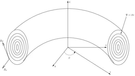
The Grad-Shafranov equation [3, 4, 5] is a rewriting of Eqs. (1-3) un-der the axisymmetric assumption. Consiun-der the cylindrical coordinate
sys-tem (er, eφ, ez). The magnetic field B is supposed to be independent of the
toroidal angle φ. Let us decompose it in a poloidal field Bp = Brer+ Bzez
and a toroidal field Bφ= Bφeφ (see Fig. 1).
Let us also introduce the poloidal flux
ψ(r, z) = 1 2π Z D Bds= Z r 0 Bzrdr
x r y z Ψ = cte φ BP Bφ
Figure 1: Toroidal geometry.
where D is the disc having as circumference the circle centered on the Oz axis and passing through a point (r, z) in a poloidal section. From Eq. (2)
one deduces that Bp =
1
r[∇ψ × eφ]. Therefore B.∇ψ = 0 meaning that ψ is
a constant on each magnetic surface and that p = p(ψ).
The same poloidal-toroidal decomposition can be applied to j. From Eq.
(1) it is clear that ∇ · j = 0. As for Bp it is shown that there exists a function
f , called the diamagnetic function, such that jp =
1
r[∇(
f
µ0) × e
φ]. Since
j.∇p = 0 then ∇f × ∇p = 0 and f is constant on the magnetic surfaces,
f = f (ψ).
From Eq. (1) one also deduces that Bφ=
f reφand jφ = (−∆ ∗ψ)e φwhere ∆∗. = ∂ ∂r( 1 µ0r ∂. ∂r) + ∂ ∂z( 1 µ0r ∂. ∂z). To sum up
B= Bp+ Bφ Bp = 1 r[∇ψ × eφ] Bφ= f reφ and j= jp+ jφ jp = 1 r[∇ f µ0 × e φ] jφ = −∆∗ψeφ
From Eq. (3) one deduces that
(jp+ jφeφ) × (Bp+ Bφeφ) = − 1 µ0r Bφ∇f + jφ 1 r∇ψ = ∇p and since ∇p = p′(ψ)∇ψ and ∇f = f′(ψ)∇ψ
the Grad-Shafranov equation valid in the plasma reads
−∆∗ψ = rp′(ψ) + 1
µ0r
(f f′)(ψ) (4)
Thus under the axisymmetric assumption, the three dimensional equilib-rium Eqs. (1 - 3) reduce to a two dimensional non linear problem. Note that
the right-hand side of Eq. (4) represents the toroidal component jφ of the
current density in the plasma which is determined by the unknown functions
p′ and f f′. In the vacuum there is no current and the poloidal flux satisfies
−∆∗ψ = 0
In this paper, we are interested in the numerical reconstruction of the equilibrium i.e of the poloidal flux ψ and in the identification of the unknown plasma current density [6, 7, 8]. In a control perspective this reconstruction has to be achieved in real time from experimental measurements. The main
difficulty consists in identifying the functions p′ and f f′ in the non linear
right-hand side source term in Eq. (4). An iterative strategy involving a finite element method for the resolution of the direct problem and a least square optimisation procedure for the identification of the non linearity using a decomposition basis is proposed.
Let us give a brief historical background of this problem of the recon-struction of the plasma current density from experimental measurements. In large aspect ratio Tokamaks with circular cross-sections, it was established
in [9, 10] that the quantities that can be identified from magnetic
measure-ments are the total plasma current Ip and a sum involving the poloidal beta
and the internal inductance: βp+ li/2 (see Appendix C). A large number of
papers proved the possibility of separating βp from li as soon as the plasma is
no longer circular with high-aspect ratio [11, 12, 13, 14]. The fact of adding supplementary experimental diagnostics, such as line integrated electronic density and Faraday rotation measurements, has considerably improved the identification of the current density profile [15, 6, 7]. The knowledge of the flux lines (from density or temperature measurements) enables in principle
[16] to determine fully the two functions p′ and f f′ in the toroidal plasma
current density, except in a particular case pointed out by [17] and studied by [18] and referred to as minimum-B equilibria. The difficulty in the recon-struction of the current profile, especially when only magnetic measurements are used, has been pointed out in [19] and is inherent to the ill-posedness of this inverse problem. The theory of variances in equilibrium reconstruction [20] enables to determine by statistical methods what kind of plasma func-tions can be reconstructed in a robust way. The equilibrium reconstruction problem in the case of anisotropic pressure is treated in [21].
A certain number of mathematical results on the identifiability of the right-hand-side of the Grad-Shafranov equation from Cauchy boundary con-ditions on the plasma frontier exist and seem unknown from the physical community. They are first dealing with the cylindrical case where the
equi-librium equation becomes −∆ψ = p′(ψ) and where only one non-linearity
has to be identified. It is clear that, if the plasma boundary is circular, then the magnetic field is constant on the plasma boundary and there is an infinity of non-linearities giving this value and the only information coming from the poloidal field on the plasma boundary is the total plasma current. In [22]
it was proved that if p′ is a real-analytic function, then in a domain with
a corner there is only one non-linearity p′ corresponding to a given poloidal
field on the plasma boundary. Some angles in the proof were excluded but in [23] the proof was given for corners with arbitrary angles (including the 90 degrees X-point case). Curiously the case where the plasma boundary is smooth is mathematically more difficult and it has been proved in [24] that,
if the plasma is non-circular and if p′ is affine in terms of ψ then there
ex-ists at most a finite number of affine functions corresponding to the Cauchy boundary conditions. The link with the Schiffer and Pompeiu conjectures which is clearly pointed out in this paper is particularly interesting. In [25] results of unicity for a class of affine functions or for exponential functions are
given for special smooth boundaries and results of non-unicity for doublet-type configurations. Finally in [26] identifiability results are given for the full Grad-Shafranov equation in a domain with a corner, with some excep-tions for the angle. Of course, in spite of all these identifiability results, the ill-posedness of the reconstruction of the non-linearities from the Cauchy boundary measurements remains and has to be tackled very cautiously.
Section 2 is devoted to the statement of the mathematical problem and to the description of the experimental measurements avalaible. The proposed algorithm is described in Section 3. This methodology has been implemented in a software called Equinox and numerical results using synthetic and real measurements are presented in Section 4.
2. Setting of the direct and inverse problems 2.1. Experimental measurements
Although the unknown functions p′(ψ) and (f f′)(ψ) cannot be directly
measured in a Tokamak several measurements are available:
• Magnetic measurements: they represent the basic information on which any equilibrium reconstruction relies. Flux loops provide measurements of ψ and magnetic probes provide measurements of the poloidal field
Bp at several points around the vacuum vessel. Let Ω be the domain
representing the vacuum vessel and ∂Ω its boundary. In what follows we assume that we are able to obtain the Dirichlet boundary
condi-tions ψ = gD and the Neumann boundary conditions
1 r
∂ψ
∂n = gN at
any points of the contour ∂Ω thanks to a preprocessing of the magnetic measurements. This preprocessing can either be a simple interpolation between real measurements or be the result of some boundary recon-struction algorithm which computes ψ outside the plasma satisfying
∆∗ψ = 0 under the constraint of the measurements [27, 28, 29].
A second set of measurements which can be used as a complement to magnetic measurements are internal measurements:
• Interferometric measurements: they give the values of the integrals
along a family of chords Ci of the electronic density ne(ψ) which is
approximately constant on each flux line Z
Ci
• Polarimetric measurements: they give the value of the integrals Z Ci ne(ψ) r ∂ψ ∂ndl = αi. ∂ψ
∂n is the normal derivative of ψ along the chord Ci.
Even when using magnetic measurements only for the equilibrium recon-struction the numerical algorithm presented in this paper also uses:
• Current measurement: it gives the value of the total plasma current Ip
defined by
Ip =
Z
Ωp
jφdx.
Ampere’s theorem shows that this quantity can be deduced from mag-netic measurements.
• Toroidal field measurement: it gives the value B0 of the toroidal
com-ponent of the field in the vacuum at the point (R0, 0) where R0 is the
major radius of the Tokamak. This is used for the integration of f f′
into f and for the computation of the safety factor q (see Appendix A). 2.2. Direct problem
The equilibrium of a plasma in a Tokamak is a free boundary problem. The plasma boundary is determined either as being the last flux line in a limiter L or as being a magnetic separatrix with an X-point (hyperbolic
point). The region Ωp ⊂ Ω containing the plasma is defined by
Ωp = {x ∈ Ω, ψ(x) ≥ ψb}
where ψb = maxLψ in the limiter configuration or ψb = ψ(X) when an
X-point exists.
In the vacuum region, the right-hand side of Eq. (4) vanishes and the equilibrium equation reads
∆∗ψ = 0 in Ω \ Ωp
Let us introduce the normalized flux ¯ψ = ψ − ψa
ψb− ψa ∈ [0, 1] in Ωp with ψa = maxΩpψ, A( ¯ψ) = R0 λ p ′(ψ) and B( ¯ψ) = 1 λµ0R0 (f f′)(ψ). This is
defined and identified on the fixed interval [0, 1]. Imposing Dirichlet bound-ary conditions the final equilibrium equation is expressed as the boundbound-ary value problem: −∆∗ψ = λ[ r R0 A( ¯ψ) + R0 r B( ¯ψ)]χΩp in Ω ψ = gD on ∂Ω (5)
The free boundary aspect of the problem reduces to the particular non
linear-ity appearing through χΩp the characteristic function of Ωp. The parameter
λ is a scaling factor used to ensure that the given total current value Ip is
satisfied Ip = λ Z Ωp [ r R0 A( ¯ψ) +R0 r B( ¯ψ)]dx. (6) 2.3. Inverse problem
The inverse problem consists in the identification of functions A and B from the measurements available. It is formulated as a least-square mini-mization problem ( Find A∗, B∗, n∗ e such that : J(A∗, B∗, n∗ e) = inf J(A, B, ne). (7) If magnetic measurements only are used the formulation only needs the
A and B variables and the J1 and J2 terms in Eq. (8) below are not needed.
When polarimetric and interferometric measurements are used, the electronic
density ne( ¯ψ) also has to be identified even if it does not appear in Eq. (5).
The cost function J is defined by
J(A, B, ne) = J0+ J1 + J2+ Jε (8)
J0 describes the misfit between computed and measured tangential
compo-nent of Bp J0 = 1 2 N X k=1 (wk)2( 1 r ∂ψ ∂n(Mk) − gN(Mk)) 2
where N is the number of points Mkof the boundary ∂Ω where the magnetic
J1 = 1 2 Nc X k=1 (wpolark )2 ( Z Ck ne( ¯ψ) r ∂ψ ∂ndl − αk) 2 and J2 = 1 2 Nc X k=1 (wkinter)2( Z Ck ne( ¯ψ)dl − γk)2
Nc is the number of chords over which interferometry and polarimetry
measurements are given. The weights w give the relative importance of the different measurements used. The influence of the choice of the weights on the results of the identification was extensively studied in [7]. As a
conse-quence of the ill-posedness of the identification of A, B and ne, a Tikhonov
regularization term Jε is introduced [30] where
Jε = εA 2 Z 1 0 [A′′(x)]2 dx + εB 2 Z 1 0 [B′′(x)]2 dx +εne 2 Z 1 0 [n′′e(x)]2 dx
and εA, εB and εne are the regularization parameters.
The values of the different weights and parameters introduced in the cost function are discussed in Section 4.
It should be noticed here that magnetic measurements provide Dirichlet and Neumann boundary conditions. The choice was made to use the Dirichlet boundary conditions in the resolution of direct problem and to include the Neumann boundary conditions in the cost function formulated to solve the inverse problem. This is arbitrary and another solution could have been chosen.
3. Algorithm and numerical resolution 3.1. Overview of the algorithm
The aim of the method is to reconstruct the equilibrium and the toroidal current density in real time. At each time step determined by the avail-ability of new measurements during a discharge, the algorithm consists in
constructing a sequence (ψn, Ωn
p, An, Bn, λn) converging to the solution
vec-tor (ψ, Ωp, A, B, λ). The unknown function ne may be added too if
interfer-ometry and polarimetry measurements are used. The sequence is obtained through the following iterative loop:
• Starting guess: ψ0, Ω0
p, A0, B0 and λ0 known from the previous time
step solution.
• Step 1 - Optimisation step: compute λn+1 satisfying (6)
λn+1= Ip/ Z Ωn p [ r R0 An( ¯ψn) + R0 r B n( ¯ψn)]dx
then compute An+1( ¯ψn) and Bn+1( ¯ψn) using the least square procedure
detailed in Section 3.2.2.
• Step 2 - Direct problem step: compute ψn+1 solution to
−∆∗ψn+1 = λn+1[ r R0 An+1( ¯ψn) + R0 r B n+1( ¯ψn)]χ Ωn p in Ω ψn+1 = g D on ∂Ω. (9)
and the new plasma domain Ωn+1
p .
• n := n + 1. If the process has not converged return to Step 1 else
(ψ, Ωp, A, B, λ) = (ψn, Ωnp, An, Bn, λn). The process is supposed to have
converged when the relative residu ||ψ
n+1− ψn||
||ψn|| is small enough.
At each iteration of the algorithm, an inverse problem corresponding to the optimization step and an approximated direct Grad-Shafranov problem
have to be solved successively. In Eq. (9), ¯ψn is known and since the
right-hand side does not depend on ψn+1 the boundary value problem (9) is linear.
In the next section the numerical methods used to solve the two problems corresponding to step 1 and step 2 are detailed.
3.2. Numerical resolution
3.2.1. The finite element method for the direct problem
The resolution of the direct problem is based on a classical P1
finite
element method [31]. Let us consider the family of triangulation τh of Ω, and
Vh the finite dimensional subspace of H1(Ω) defined by
and introduce V0
h = Vh∩ H01(Ω). The discrete variational formulation of the
boundary value problem (9) reads
Find ψh∈ Vh with ψh = gD on ∂Ω such that
∀vh ∈ Vh0, Z Ω 1 µ0r∇ψ h· ∇vhdx = Z Ωp λ[ r R0 A( ¯ψ∗) + R0 r B( ¯ψ ∗)]v hdx (10)
where ψ∗ represents the known value of ψ at the previous iteration.
Nu-merically the Dirichlet boundary conditions are imposed using the method
consisting in computing the stiffness matrix ˆK of the Neumann problem and
modifying it. Consider (vi) a basis of Vh then ˆKij =
Z
Ω
1
µ0r∇v
i∇vjdx The
modifications consist in replacing the rows corresponding to each boundary node setting 1 on the diagonal terms and 0 elsewhere. At each iteration only the right-hand side of the linear system in which the Dirichlet boundary con-ditions appear has to be modified. The linear system corresponding to Eq. (10) can be written in the form
K.Ψ = y + g (11)
where K is the n × n modified stiffness matrix, Ψ is the unknown vector of size n (the number of nodes of the finite elements mesh), y is the vector associated with the modified right-hand side of Eq. (10) and g is the vector corresponding to the Dirichlet boundary conditions.
The matrix K is sparse and let LU be its decomposition. The inverse
matrix K−1 is not sparse. The linear system (11) is inverted using the LU
decomposition since it is computationally cheaper than using the full inverse
matrix K−1 which is nevertheless needed for the optimization step of the
algorithm in Eq. (15) below.
The vector y depends on functions A and B which are determined in
the optimization step. Functions A, B and ne are decomposed on a finite
dimensional basis (Φi)i=1,...,mof functions defined on [0, 1]
A(x) = m X i aiΦi(x), B(x) = m X i biΦi(x) and ne(x) = m X i ciΦi(x).
The vector y reads
where u = (a1, ..., am, b1, ..., bm) ∈ R2m is the vector of the components of
functions A and B in the basis (Φi). The matrix Y of size n × 2m is defined
as follows. Each row i of Y is decomposed as
Yij( ¯Ψ∗) = Z Ωp λ r R0 Φj( ¯ψ∗)vidx if 1 ≤ j ≤ m Z Ωp λR0 r Φj−m( ¯ψ ∗)v idx if m + 1 ≤ j ≤ 2m.
3.2.2. Detailed numerical algorithm
One equilibrium computation corresponds to one instant in time during a pulse. The quasi-static approximation consists in considering that at each instant the Grad-Shafranov equation is satisfied. During a pulse successive equilibrium configurations are computed with a time resolution ∆t corre-sponding to the acquisition time of measurements:
• Initialization before the discharge: the modified stiffness matrix K, its
LU decomposition as well its inverse K−1 are computed once for all
and stored.
• Consider that the equilibrium at time t − ∆t is known and that a new set of measurements is acquired at time t.
• Computation of the new equilibrium at time t through the iterative loop briefly described in the previous Section and detailed below: The equilibrium from the previous time step is used as a first guess in the iterative loop.
Step 1 - Optimization step. During the optimisation step, neis first estimated
from interferometric measurements and A and B are computed in a second time.
• Compute the electronic density ne based on the equilibrium of the
previous iteration ¯ψ∗ using a least square formulation for the minimun
of J2 with Tikhonov regularization and solving the associated normal
equation: The flux ¯ψ∗ is given.
ne(x) =
m
X
j=1
The interferometric measurements for i = 1 ... nc are γi ≈ Z Ci ne( ¯ψ∗)dl = X j vj Z Ci φj( ¯ψ∗)dl = X j vjBij
The cost functional reads
J(v) = 1 2 X i (wiinter)2(X j Bijvj − γi)2+ ε 2v TΛv = 1 2||D 1/2 (Bv − γ)||2 + ε 2v TΛv
where D1/2 = diag(winter
i ) and the regularization matrix Λ is defined
by Λij = Z 1 0 Φ”i(x)Φ”j(x)dx and Φ”
i is the second order derivative of the basis function Φi.
It is minimized solving the associated normal equation
(α2(D1/2B)T(D1/2B) + ˆεΛ)ˆv = α(D1/2B)TD1/2γ (13)
Since ne ≈ 1019m−3 an adimensionalizing parameter α = 1019m−3,
such that v = αˆv, is introduced in order to precondition the linear
system which is inverted using LU decomposition, as well as a reason-able prescribed value for the non dimensional regularization parameter ˆ
ε = α2ε.
• Compute λn+1 satisfying Eq. (6). In the right-hand side y, λ appears
in the product λu. In order to avoid any divergence issue due to the
non uniqueness of λ (for all α, λu = (λα)(u
α)) the degrees of freedom
(dofs) u are scaled by m = max(|ai|), u is replaced by
1
mu and λ by
mλ.
• Compute A and B. In order to approximate A and B, suppose ne is
known and consider the discrete approximated inverse problem ( Find u minimizing : J(u) = 1 2kC(ψ ∗ )Ψ − dk2D + ε 2u TΛu (14)
where C(ψ∗) is the observation operator and d the vector of
experimen-tal measurements. The first term in J is the discrete version of J0+ J1.
The second one corresponds to the first two terms of the Tikhonov
reg-ularization Jε with εA= εB = ε which will always be assumed in order
for functions A and B to play a symmetric role.
Let us denote by l the number of measurements available (l = N + Nc
if magnetic and polarimetric measurements are used) and by D the
diagonal matrix made of the weights wk and wkpolar, the norm k.kD is
defined by ∀x ∈ Rl kxk2
D = (Dx, x) = (D1/2x, D1/2x)
C(ψ∗) is a sparse matrix of size l × n and can be viewed as a vector
composed of two blocks C0 of size N × n and independent of ψ∗ and
C1(ψ∗) of size Nc × n corresponding respectively to J0 and J1. That
is to say that multiplication of the kth row of C0 by ψ gives the kth
Neumann boundary condition approximation
(C0)kΨ ≈ (
1 r
∂ψ
∂n)(Mk).
The block C1(ψ∗) depends on ψ∗ through the ne(ψ∗) function. The
multiplication of the kth row of C1(ψ∗) by Ψ gives the kth polarimetric
measurements approximation (C1(ψ∗))kΨ ≈ Z ck ne(ψ∗) r ∂ψ ∂ndl.
The matrix Λ is of size 2m × 2m and is block diagonal composed of
two blocks Λ1 and Λ2 of size m × m, with
(Λ1)ij = (Λ2)ij =
Z 1
0
Φ”i(x)Φ”j(x)dx
Using Eqs .(11 - 12) problem (14) becomes
J(u) = 1 2kC(ψ ∗ )Ψ − dk2D+ ε 2u TΛu = 1 2kC(ψ ∗)K−1Y ( ¯ψ∗)u + (C(ψ∗)K−1 g − d)k2 D + ε 2u TΛu = 1 2kEu − fk 2 D+ ε 2u TΛu
where E = C(ψ∗)K−1Y ( ¯ψ∗) and f = −C(ψ∗)K−1h + d. Setting ˜E =
D1/2E, problem (14) reduces to solve the normal equation
( ˜ETE + εΛ)u = ˜˜ ETf (15)
whose solution is denoted by u∗.
Step 2 - Direct problem step.. Update the dofs u and update the flux ψ by
solving the linear system
Kψ = Y ( ¯ψ∗)u∗+ g (16)
using the LU decomposition of matrix K. Update Ωp possibly computing
the position of the X-point if the plasma is not in a limiter configuration. Finally it should be noticed that this algorithm is particularly well adapted to real-time applications. Indeed during the computations the expensive operations are the updates of matrices C and Y as well as the computation
of products CK−1 and CK−1Y which appear in Eq. (15). In order to reduce
computation time the K−1 matrix is precomputed and only the ψ-dependent
part of C is dealt with. The resolution of the direct problem, Eq. (16), is cheap since the LU decomposition of the K matrix is also precomputed. 4. Numerical results
4.1. Twin experiment with noise free magnetic measurements
In this section we assume that the poloidal flux corresponding to an equi-librium configuration ψ is given on the boundary Γ . These Dirichlet bound-ary conditions can either be real measurements or can be the output from some equilibrium simulation code. In a first step we also assume to know
functions p′ and f f′ (or A and B). In what follows these reference functions
are given point by point. It is then possible to run a direct simulation to
compute ψ on Ω (see Fig. 2) and thus 1
r ∂ψ
∂n on Γ which can then be used as
measurements in an inverse problem resolution.
In this first experiment the magnetic measurements are free of noise. The identification algorithm is initialized using the first guess functions are A(x) = B(x) = 1−x and λ = 1. The poloidal flux ψ is initially a constant on
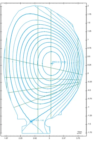
1.87 2.25 2.62 3 3.37 3.75 -1.75 -1.5 -1.25 -1 -0.75 -0.5 -0.25 0 0.25 0.5 0.75 1 1.25 1.5 1.75 2 10cm MAG (3.1, 0.31) XPL (2.5, -1.4)
Figure 2: An equilibrium configuration for the tokamak JET from which twin experiments are performed. The domain Ω and its boundary Γ (blue line) are shown. Isoflux are plotted from ¯ψ = 0 (magnetic axis) to ¯ψ = 1 (plasma boundary defined by the existence of an X-point at point r = 2.5 and z = −1.4 m) by step of ∆ ¯ψ = 0.1 Interferometry and polarimetry chords appear in green.
measurements are defined by wk =
1 √
Nσ. Since the error on magnetic
measurements are of about one percent we define σ = 0.01Bm where Bm is a
mean magnetic field value which thanks to Ampere’s theorem can be defined
as Bm =
µ0Ip
|Γ| .
The functions A and B are decomposed in a function basis defined on the interval [0, 1]. Several basis have been tested (piecewise affine functions,
polynomials, B-splines and wavelets) in order to verify that the result of the identification does not depend on the decomposition basis. This is the case as long as the dimension of the basis is large enough. In the remaining part of this paper each function is decomposed in the same basis of 8 B-splines [32]. The boundary condition A(1) = B(1) = 0 is imposed.
The computations are carried out for several values of the regularization
parameters ε ranging from 10−10to 1. We are interested in the ability of the
method to recover functions A and B and thus the current density profile averaged over the magnetic surfaces (see Appendix A):
R0 < j(r, ¯ψ) r >= λA( ¯ψ) + λR 2 0 < 1 r2 > B( ¯ψ)
and the safety factor q (see Appendix B).
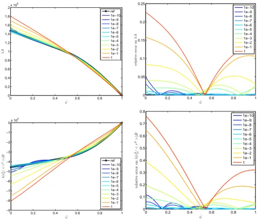
As can be seen from Fig. 3 the optimal choice for ε is of about 10−5
for which functions A and B are well recovered. For smaller values some oscillations appear because the regularization is not strong enough and on the contrary greater values lead to less precision in the recovery of the unknown functions since regularization is too strong. In the second column the relative errors on the identified functions are plotted.
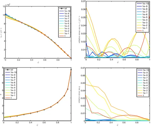
Figure 4 shows an important point. Almost whatever the chosen value of ε is, i.e. whatever the quality of the identification of A and B is, the identified
averaged current density R0 <
j(r, ¯ψ)
r > as well as the safety factor q are
always well recovered and the relative errors are one order of magnitude smaller than for functions A and B. The same kind of observation was made in [8] where the identified functions A and B seemed to be rather sensitive to perturbations whereas the averaged current density was very stable.
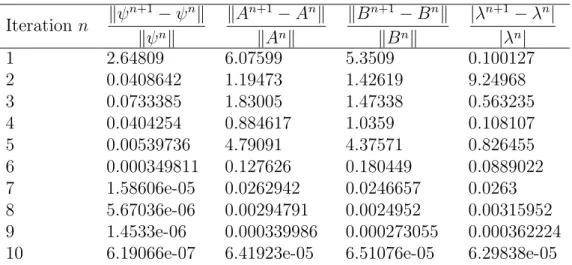
In Table 1, the evolution of the relative residu on ψ, A, B and λ versus the number of iterations is given. It demonstrates numerically the convergence
of the algorithm in this case where a value of 10−6 is used as stop condition.
The algorithm needs 10 iterations to converge. It is interesting to notice that even though the first guess is not particularly well chosen the relative residu on ψ at the second iteration has already fallen to 4%. In real applications when simulating a whole pulse the first guess for the computation of the equilibrium at t is the equilibrium computed at t − ∆t and 2 iterations are enough to ensure a good convergence of the algorithm.
0 0.2 0.4 0.6 0.8 1 0 0.2 0.4 0.6 0.8 1 1.2 1.4 1.6 1.8 2x 10 6 ¯ ψ λ A ref 1e−10 1e−9 1e−8 1e−7 1e−6 1e−5 1e−4 1e−3 1e−2 1e−1 1 0 0.2 0.4 0.6 0.8 1 0 0.05 0.1 0.15 0.2 0.25 ¯ ψ re la ti v e er ro r on λ A 1e−10 1e−9 1e−8 1e−7 1e−6 1e−5 1e−4 1e−3 1e−2 1e−1 1 0 0.2 0.4 0.6 0.8 1 −9 −8 −7 −6 −5 −4 −3 −2 −1 0x 10 5 ¯ ψ λ (r 2/0 < r 2> )B ref 1e−10 1e−9 1e−8 1e−7 1e−6 1e−5 1e−4 1e−3 1e−2 1e−1 1 0 0.2 0.4 0.6 0.8 1 0 0.1 0.2 0.3 0.4 0.5 0.6 0.7 0.8 ¯ ψ re la ti v e er ro r on λ (r 2/0 < r 2> )B 1e−10 1e−9 1e−8 1e−7 1e−6 1e−5 1e−4 1e−3 1e−2 1e−1 1
Figure 3: Twin experiment with noise free measurements and different regularization parameters ε ranging from 10−10 to 1. Left column: identified functions λA( ¯ψ) and
λR2 0 <
1
r2 > B( ¯ψ) for each different ε value, and the known reference functions. Right
column: relative errors.
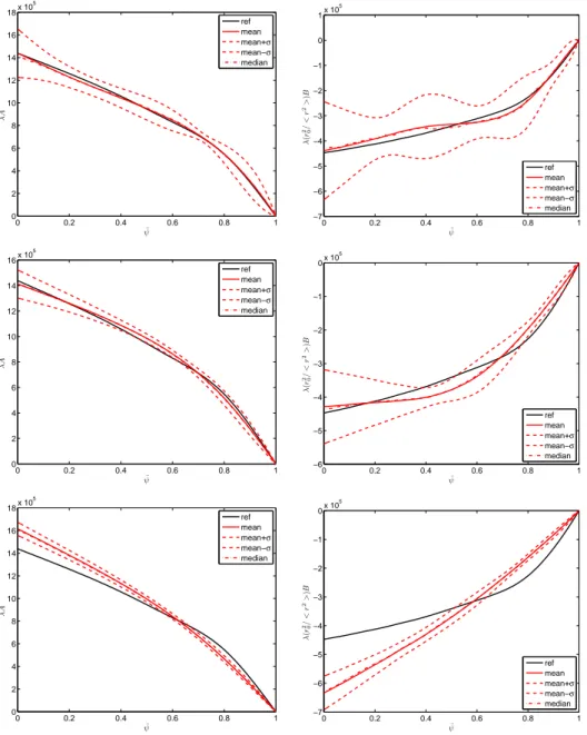
4.2. Twin experiment with noisy magnetic measurements
Figures 5 and 6 show the results of the same type of numerical experiment but with noisy measurements. Each magnetic input, m representing either ψ
or 1
r ∂ψ
∂n at a point of the domain boundary Γ, is perturbed with a one percent
noise normally distributed, mη = m + η with η ∼ N(m, 0.01m). For each
chosen value of the regularization parameter the algorithm is run 200 times with measurements randomly perturbed as above. Then for each function
λA, λR20 <
1
r2 > B, R0 <
j(r, ¯ψ)
r > and q, a mean function and a standard
0 0.2 0.4 0.6 0.8 1 0 2 4 6 8 10 12x 10 5 ¯ ψ r0 < j/ r > ref 1e−10 1e−9 1e−8 1e−7 1e−6 1e−5 1e−4 1e−3 1e−2 1e−1 1 0 0.2 0.4 0.6 0.8 1 0 0.01 0.02 0.03 0.04 0.05 0.06 0.07 ¯ ψ re la ti v e er ro r on r0 < j/ r > 1e−10 1e−9 1e−8 1e−7 1e−6 1e−5 1e−4 1e−3 1e−2 1e−1 1 0 0.2 0.4 0.6 0.8 1 1 2 3 4 5 6 7 8 ¯ ψ q ref 1e−10 1e−9 1e−8 1e−7 1e−6 1e−5 1e−4 1e−3 1e−2 1e−1 1 0 0.2 0.4 0.6 0.8 1 0 0.01 0.02 0.03 0.04 0.05 0.06 0.07 ¯ ψ re la ti v e er ro r on q 1e−10 1e−9 1e−8 1e−7 1e−6 1e−5 1e−4 1e−3 1e−2 1e−1 1
Figure 4: Twin experiment with noise free measurements and different regularization parameters ε ranging from 10−10 to 1. Left column: resulting identified averaged current
density R0 <
j(r, ¯ψ)
r >, safety factor q for each ε value and the corresponding known reference values. Right column: relative errors.
In comparison with the noise free case the regularization parameter needs
to be significantly increased to values of at least ε = 10−2 and for a safer
convergence of the algorithm to ε = 10−1. For smaller values the algorithm
either does not converge or gives very oscillating identified functions.
The mean error on the reconstructed functions is always smaller in the
interval ¯ψ ∈ [0.5, 1] than in the interval [0, 0.5]. This is due to the fact
that magnetic measurements are external to the plasma and do not provide enough information to properly reconstruct the functions in the innermost part of the plasma.
Table 1: Numerical convergence of the algorithm. Iteration n kψ n+1− ψnk kψnk kAn+1− Ank kAnk kBn+1− Bnk kBnk |λn+1− λn| |λn| 1 2.64809 6.07599 5.3509 0.100127 2 0.0408642 1.19473 1.42619 9.24968 3 0.0733385 1.83005 1.47338 0.563235 4 0.0404254 0.884617 1.0359 0.108107 5 0.00539736 4.79091 4.37571 0.826455 6 0.000349811 0.127626 0.180449 0.0889022 7 1.58606e-05 0.0262942 0.0246657 0.0263 8 5.67036e-06 0.00294791 0.0024952 0.00315952 9 1.4533e-06 0.000339986 0.000273055 0.000362224
10 6.19066e-07 6.41923e-05 6.51076e-05 6.29838e-05
functions decreases. With small ε the algorithm can find very different
func-tions depending on the perturbafunc-tions of the measurements. With ε = 10−2
the variability in the identified functions A and B is strong however the mean identified functions are close to the exact reference ones. On the other hand with ε = 1 the variability of the identified functions is strongly reduced but they are quite different from the exact reference functions in the interval [0, 0.5].
It is worth noticing that in all cases the resulting safety factor q and
av-eraged current density R0 <
j(r, ¯ψ)
r > are well recovered. The remark of
the preceding section on the identifiability of the averaged current density still holds: it is quite well recovered even if functions A and B taken sepa-rately are not well identified. The mean error on the current density profile is almost always smaller than the mean errors on functions A and B. More-over this error does not change very much between the different cases and
particularly between the ε = 10−1 and the ε = 1 cases. This implies that
for a large interval of ε the value of the part of the cost function related to
magnetic measurements J0 is almost constant. Therefore it is difficult to find
an optimal value for the regularization parameter. For example the L-curve method [33] for the determination of the regularization parameter can hardly be used and gives some results which are not very reliable since the L-curves
are not well behaved and the location of the corner is not clear. The ”L” is an almost vertical line. This is due to the fact that, in a large interval of ε values, an increase in ε implies a important decrease in the
regulariza-tion term 1
2(u
∗(ε))TΛu∗(ε) but does not lead to a significative increase in the
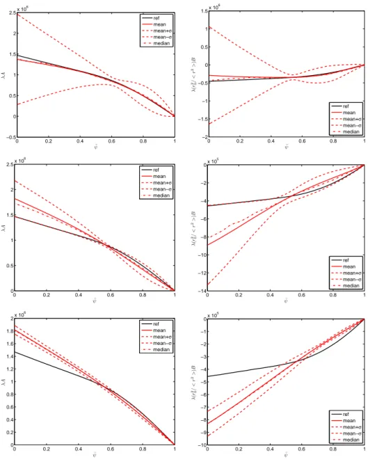
0 0.2 0.4 0.6 0.8 1 −0.5 0 0.5 1 1.5 2 2.5x 10 6 ¯ ψ λ A ref mean mean+σ mean−σ median 0 0.2 0.4 0.6 0.8 1 −2 −1.5 −1 −0.5 0 0.5 1 1.5x 10 6 ¯ ψ λ (r 2/0 < r 2> )B ref mean mean+σ mean−σ median 0 0.2 0.4 0.6 0.8 1 0 0.5 1 1.5 2 2.5x 10 6 ¯ ψ λ A ref mean mean+σ mean−σ median 0 0.2 0.4 0.6 0.8 1 −14 −12 −10 −8 −6 −4 −2 0x 10 5 ¯ ψ λ (r 2/0 < r 2> )B ref mean mean+σ mean−σ median 0 0.2 0.4 0.6 0.8 1 0 0.2 0.4 0.6 0.8 1 1.2 1.4 1.6 1.8 2x 10 6 ¯ ψ λ A ref mean mean+σ mean−σ median 0 0.2 0.4 0.6 0.8 1 −10 −9 −8 −7 −6 −5 −4 −3 −2 −1 0x 10 5 ¯ ψ λ (r 2/0 < r 2 > )B ref mean mean+σ mean−σ median
Figure 5: Statistical results of the identification experiments with noisy magnetic mea-surements. Row 1: ε = 10−2, row 2: ε = 10−1, row 3 ε = 1. Column 1: function λA( ¯ψ)
and column 2: λR2 0 <
1
r2 > B( ¯ψ). For each function the reference value from which
the unperturbed measurements were computed is given in black and the mean identified function in red. The mean ± standard deviation functions are shown in dashed red.
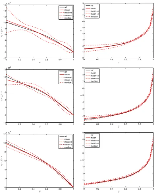
0 0.2 0.4 0.6 0.8 1 −2 0 2 4 6 8 10 12 14 16x 10 5 ¯ ψ r0 < j/ r > ref mean mean+σ mean−σ median 0 0.2 0.4 0.6 0.8 1 0 1 2 3 4 5 6 7 8 9 ¯ ψ q ref mean mean+σ mean−σ median 0 0.2 0.4 0.6 0.8 1 −2 0 2 4 6 8 10 12x 10 5 ¯ ψ r0 < j/ r > ref mean mean+σ mean−σ median 0 0.2 0.4 0.6 0.8 1 1 2 3 4 5 6 7 8 9 ¯ ψ q ref mean mean+σ mean−σ median 0 0.2 0.4 0.6 0.8 1 0 2 4 6 8 10 12x 10 5 ¯ ψ r0 < j/ r > ref mean mean+σ mean−σ median 0 0.2 0.4 0.6 0.8 1 1 2 3 4 5 6 7 8 9 ¯ ψ q ref mean mean+σ mean−σ median
Figure 6: Statistical results of the identification experiments with noisy magnetic mea-surements. Row 1: ε = 10−2, row 2: ε = 10−1, row 3 ε = 1. Column 1: R0< j(r, ¯ψ)
r >, and column 2: safety factor q. For each function the reference value is given in black and the mean identified function in red. The mean ± standard deviation functions are shown in dashed red.
4.3. Twin experiment with noisy magnetic, interferometric and polarimetric measurements
In this last twin experiment, interferometric and polarimetric
measure-ments are also used. At first a reference density profile, ne(x) is prescribed
point by point on [0, 1], as well as the same reference A and B functions as in the previous twin experiments. Then similar to the preceding section the equilibrium is computed from given Dirichlet boundary condition. A set of artificial magnetic, interferometric and polarimetric measurements is gener-ated. Finally several twin experiments with a 1% noise are performed and some statistics are computed. The weights related to interferometric and polarimetric measurements in the cost function are defined as
• wpolark =
1 √
Ncσpolar
, with σpolar = 10−1 radians
• winter k = 1 √ Ncσinter , with σinter = 1018 m−3
The determination of the regularization parameter for the density
func-tion neis far less a problem than for functions A and B since for example the
L-curve method works quite well in this case (see Fig. 10 in the next Section)
and the ne function is well recovered as shown on Fig. 9. The regularization
parameter for the density function is set to εne = 10−2.
The statistical results of the twin experiments are shown on Figs. 7 and 8 for 3 different values of ε. The use of interferometric and polarimetric mea-surements adds supplementary constraints on the A and B functions. The variability in the recovered functions is less important than in the case where
only magnetics are used particularly for ¯ψ ∈ [0, 0.5]. This is not surprising
since the new measurements are internal and bring some information con-tained inside the plasma domain. Nevertheless it is not enough to perfectly reconstruct independently the A and B functions. This does not prevent an excellent recovery of the averaged current density profile and of the safety factor q. This phenomenon already observed in the magnetics case is empha-sized here where the variability of the recovered profiles has decreased. 4.4. A real pulse
The algorithm detailed in this paper has been implemented in a C++ software called Equinox developed in collaboration with the Fusion Depart-ment at Cadarache for Tore Supra and JET. Equinox can be used on the
one hand for precise studies in which the computing time is not a limiting factor and on the other hand in a real-time framework to reconstruct the successive plasma equilibrium configurations during a whole pulse. For the time being it is used on JET and ToreSupra pulses, it has also been tested on the Tokamak TCV and can potentially be used on any Tokamak.
During the real time analysis of a whole pulse an equilibrium is recon-structed from new measurements with a time step of ∆t = 100 ms. For each equilibrium reconstruction the number of iterations of the algorithm is set to 2. This enables fast enough computations while a very good precision is achieved since the initial guess for an equilibrium computation at time t is the equilibrium computed at time t −∆t. After 1 iteration a typical value for
the relative residu on ψ is of 10−2 and it is of 10−3 after 2 iterations. Table
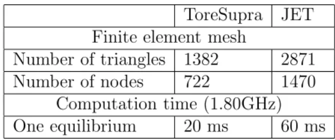
2 gives the size of the finite elements mesh used at ToreSupra and at JET as well as typical computation times on a laptop computer.
ToreSupra JET
Finite element mesh
Number of triangles 1382 2871
Number of nodes 722 1470
Computation time (1.80GHz)
One equilibrium 20 ms 60 ms
Table 2: Typical mesh size and computation time for ToreSupra and JET
The choice of the regularization parameters is crucial since it determines the balance between the fit to the data and the regularity of the identified functions. It is also difficult as is shown in the preceding section. Ideally they should be determined for each equilibrium reconstruction. However this is not possible in a real-time application and the regularization parameters have to be set apriori to a constant value. From the twin experiments presented in the preceding sections it is quite clear that a good value for the regularization
parameter ε is in the range [10−2, 1]. By trial and error on different pulses
using magnetics, interferometry and polarimetry, it appeared that a value of
ε = 5.10−2 gave good results.
As for the identification of functions A and B the choice of a good
reg-ularization parameter for the identification of ne is crucial. However in this
case the L-curve method works quite well and it was used to determine the
shots. The obtained values showed little variation and the choice of a mean value ε = 0.01 proved to be efficient. Figure 10 shows an example of an
L-curve computed for the identification of ne.
Concerning real pulses at JET we refer to [34, 35] in which a validation of Equinox is performed using many different pulses. This validation includes a posteriori comparison of the position of rational q surfaces computed from Equinox and deduced from soft X-rays measurements. The validation is satisfactory and shows again that when solving the inverse problem the use of interferometry, polarimetry and even Motional Strak Effect measurements at JET improves the location of rational q surfaces.
Here we only present an example of the output from Equinox on a Tore-Supra pulse. Figure 11 shows the equilibrium computed at time 20.408 sec-onds for ToreSupra pulse number 36182 using magnetic measurements as well as interferometric and polarimetric measurements. One can observe the po-sition of the plasma in the vacuum vessel. Isoflux lines are displayed from the magnetic axis to the boundary. The interferometry and polarimetry chords are displayed. For each chord the error between computed and measured interferometry is given in purple. These errors are about 1% for the active chords. The polarimetry absolute errors are given in yellow. Different graphs are plotted on the left hand side of the display. On the first row the identified
function A, and corresponding functions p′ and p. On the second row the
identified function B and corresponding function f f′. The third row gives
the toroidal current density jφ in the equatorial plane and the fourth one
shows the safety factor q. Finally on the fifth row the identified ne function
is plotted.
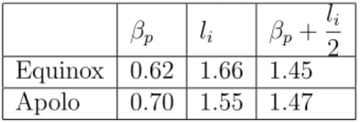
It is of importance to compute the kinetic energy poloidal βp parameter
and the internal inductance li. In Equinox these equilibrium parameters are
computed following the equations of Appendix C. For ToreSupra they are computed in the code Apolo [28] from the Shafranov integrals and from the toroidal plasma flux. The agreement between the two methods is good as
shown in Table 3. The relative errors on βp and li are about 10% while it is
of about 1% on the sum βp+
li
2.
Finally it should be noticed that at ToreSupra or JET there does not exist reliable enough pressure measurements to be used in an inverse
equi-librium reconstuction. The electron pressure pe can be reasonably estimated
from interferometry for the density ne and Thomson scattering and Electron
un-βp li βp+
li
2
Equinox 0.62 1.66 1.45
Apolo 0.70 1.55 1.47
Table 3: βp and li computed by Equinox and by Apolo for ToreSupra shot 36182 at
t=20.408s
certainties on the ion quantities ni and Ti make the ion pressure pi and thus
the total pressure p = pe+ pi unusable in a real-time identification algorithm
such as the one presented here. Moreover the quantity really important in
order to constrain the identification of the p′ term would be the pressure
gradient on which the error bars are even larger. 5. Conclusion
We have presented an algorithm for the identification of the current den-sity profile in the Grad-Shafranov equation and the equilibrium reconstruc-tion from experimental measurements in real time. We have shown thanks to several twin experiments that even though the unknown functions A and
B (or p′ and f f′) taken separately might not be always exactly identified the
resulting averaged current density and safety factor seem to be always well identified. We have also shown that the use of internal polarimetric mea-surements improves the quality of the identification but is still not enough to perfectly identify both A and B. Finally we have introduced the software Equinox in which this methodology is developed. This work constitutes a step towards the real-time control of the safety factor and of the averaged current density profile in a Tokamak plasma which will be essential in nuclear fusion reactors.
Aknowledgements
The authors are grateful to Kristoph Bosak who developed a first version of the code Equinox. Although it has now been thoroughly modified this version was an essential basis to start from.
The authors would also like to thank all colleagues from the CEA at Cadarache in France involved in a collaboration between the University of Nice and the
CEA through the LRC (Laboratoire de Recherche Conventionn´e). Discus-sions with Francois Saint-Laurent and Sylvain Bremond were particularly helpful. Emmanuel Joffrin initiated the real-time approach and Didier Ma-zon helped introducing us at JET where different people are also involved. In particular Luca Zabeo provided magnetic input data from the boundary code Xloc for Equinox and the work of Fabio Piccolo and Robert Felton is essential to implement Equinox on JET real-time system.
0 0.2 0.4 0.6 0.8 1 0 2 4 6 8 10 12 14 16 18x 10 5 ¯ ψ λ A ref mean mean+σ mean−σ median 0 0.2 0.4 0.6 0.8 1 −7 −6 −5 −4 −3 −2 −1 0 1x 10 5 ¯ ψ λ (r 2/0 < r 2> )B ref mean mean+σ mean−σ median 0 0.2 0.4 0.6 0.8 1 0 2 4 6 8 10 12 14 16x 10 5 ¯ ψ λ A ref mean mean+σ mean−σ median 0 0.2 0.4 0.6 0.8 1 −6 −5 −4 −3 −2 −1 0x 10 5 ¯ ψ λ (r 2/0 < r 2> )B ref mean mean+σ mean−σ median 0 0.2 0.4 0.6 0.8 1 0 2 4 6 8 10 12 14 16 18x 10 5 ¯ ψ λ A ref mean mean+σ mean−σ median 0 0.2 0.4 0.6 0.8 1 −7 −6 −5 −4 −3 −2 −1 0x 10 5 ¯ ψ λ (r 2/0 < r 2> )B ref mean mean+σ mean−σ median
Figure 7: Statistical results of the identification experiments with noisy measurements (magnetics, interferometry and polarimetry). Row 1: ε = 10−2, row 2: ε = 10−1, row 3
ε= 1. Column 1: function λA( ¯ψ), and column 2: λR2 0 <
1
r2 > B( ¯ψ). For each function
the reference value from which the unperturbed measurements were computed is given in black and the mean identified function in red. The mean ± standard deviation functions are shown in dashed red.
0 0.2 0.4 0.6 0.8 1 −2 0 2 4 6 8 10 12x 10 5 ¯ ψ r0 < j/ r > ref mean mean+σ mean−σ median 0 0.2 0.4 0.6 0.8 1 1 2 3 4 5 6 7 8 9 ¯ ψ q ref mean mean+σ mean−σ median 0 0.2 0.4 0.6 0.8 1 0 2 4 6 8 10 12x 10 5 ¯ ψ r0 < j/ r > ref mean mean+σ mean−σ median 0 0.2 0.4 0.6 0.8 1 1 2 3 4 5 6 7 8 9 ¯ ψ q ref mean mean+σ mean−σ median 0 0.2 0.4 0.6 0.8 1 0 2 4 6 8 10 12x 10 5 ¯ ψ r0 < j/ r > ref mean mean+σ mean−σ median 0 0.2 0.4 0.6 0.8 1 1 2 3 4 5 6 7 8 9 ¯ ψ q ref mean mean+σ mean−σ median
Figure 8: Statistical results of the identification experiments with noisy measurements (magnetics, interferometry and polarimetry). Row 1: ε = 10−2, row 2: ε = 10−1, row 3
ε= 1. Column 1: R0 <
j(r, ¯ψ)
r >, and column 2: safety factor q. For each function the reference value is given in black and the mean identified function in red. The mean ± standard deviation functions are shown in dashed red.
0 0.2 0.4 0.6 0.8 1 0 1 2 3 4 5 6x 10 19 ¯ ψ ne ref mean mean+σ mean−σ median
Figure 9: Statistical results for the identification of the density function ne with noisy
interferometric measurments. −4 −3.5 −3 −2.5 −2 −1.5 −1 −4 −3 −2 −1 0 1 2 3 residual term regularization term L−curve Corner located at εne = 0.01
Figure 10: Typical Lcurve for the determination of εne. It is a plot of the parametric
curve x(εne) = log( 1 2||D 1/2(Bv∗(ε ne) − γ)|| 2 ), y(εne) = log( 1 2(v∗(εne)) TΛv∗(ε ne)) where v∗(ε
Figure 11: Graphical output from Equinox. Reconstructed equilibrium at time 20.408 s for ToreSupra pulse number 36182. Magnetic, interferometry and polarimetry measurments are used. See text for more details.
A. Average over magnetic surfaces
The method of averaging over the magnetic surfaces is detailed in [14] (p 242). The average < A > of an arbitrary quantity A on a magnetic surface S is defined as < A >= ∂ ∂V Z V AdV
where V is the volume inside S. This notion of average has the following property: < A >= Z Cψ¯ Adl Bp Z Cψ¯ dl Bp
where Cψ¯ is a closed contour ¯ψ = cte ∈ (0, 1) and Bp = 1
r||∇ψ||.
B. Safety factor q
The safety factor is so called because of the role it plays in determining stability ([1] p 111). It can be seen as the ratio of the variation of the toroidal angle needed for one magnetic field line to perform one poloidal turn.
q = ∆φ
2π
Since q is the same for all magnetic field lines on a magnetic surface it is
a function of ψ (or ¯ψ). The expression of q used for computations is the
following q( ¯ψ) = 1 2π Z Cψ¯ Bφ rBp dl
where Cψ¯ is a closed contour ¯ψ = cte ∈ (0, 1), Bφ= f
r and f (ψ) = s (B0R0)2+ Z ψ ψb (f2 )′(y)dy
C. Poloidal βp and Internal inductance li
The full 3D plasma domain is denoted by D. The plasma domain in
the poloidal section by Ωp and its boundary ∂Ωp = Γp. Let us define Rg =
1
2(Rlef t+ Rright)
Surface and perimeter of a poloidal section. Let us define Sp = RΩpds and
Lp =
R
Γpdl. For a circular plasma of radius a: Lp = 2πa, Sp = πa
2
and
Sp =
L2
p
4π. Even for non-circular plasma the following quantity is used:
ˆ Sp = L2 p 4π (17) Plasma volume. Vp = Z D dv = Z 2π 0 Z Ωp rdφds = 2π Z Ωp rds (18)
The following approximation can be used: ˆ
Vp = 2πRgSˆp (19)
Poloidal βp. The ratio β =
p
B2/2µ
0
represents the efficiency of the con-finement of the plasma pressure by the magnetic field. The poloidal beta is defined as the ratio of the mean kinetic pressure of the plasma to its magnetic pressure ([1] p 116): βp = ¯ p B2 pa/2µ0 (20) where ¯ p = R Dpdv R Ddv = R Ωpprds R Ωprds (21) and Bpa = R ΓpBpdl R Γpdl = µ0Ip Lp (22) Let us define the internal kinetic energy
W = 3
2 Z
D
We have W = 3 2pV¯ p = 3 2 B2 pa 2µ0 Vpβp
and from Eq. (22), (19) and (17) follows that ([1] p 504)
W = 3
8µ0RgI
2 pβb
Then βp can be approximated by
βp = 3 2pV¯ p 3 8µ0RgI 2 p (23)
which the default βp computed by Equinox.
C.1. Internal inductance li
The internal inductance li of the plasma characterizes the current density
profile ([1] p 120, [14] p 44): li = ¯ B2 p B2 pa (24) where ¯ Bp2 = R DB 2 pdv R Ddv
In Equinox the computation of li is done as follows:
li = ¯ B2 pVp B2 paVp
Using Eq. (22), Eq. (19) and Eq. (17) leads to
li = ¯ B2 pVp µ2 0 2 RgI 2 p (25)
References
[1] J. Wesson, Tokamaks, Vol. 118 of International Series of Monographs on Physics, Oxford University Press Inc., New York, Third Edition, 2004. [2] H. Grad, J. Hogan, Classical diffusion in a tokomak, Physical review
letters 24 (24) (1970) 1337–1340.
[3] H. Grad, H. Rubin, Hydromagnetic equilibria and force-free fields, in: 2nd U.N. Conference on the Peaceful uses of Atomic Energy, Vol. 31, Geneva, 1958, pp. 190–197.
[4] V. Shafranov, On magnetohydrodynamical equilibrium configurations, Soviet Physics JETP 6 (3) (1958) 1013.
[5] C. Mercier, The MHD approach to the problem of plasma confinement in closed magnetic configurations, Lectures in Plasma Physics, Commission of the European Communities, Luxembourg, 1974.
[6] L. Lao, J. Ferron, R. Geoebner, W. Howl, H. St. John, E. Strait, T. Tay-lor, Equilibrium analysis of current profiles in Tokamaks, Nuclear Fusion 30 (6) (1990) 1035.
[7] J. Blum, E. Lazzaro, J. O’Rourke, B. Keegan, Y. Stefan, Problems and methods of self-consistent reconstruction of tokamak equilibrium profiles from magnetic and polarimetric measurements, Nuclear Fusion 30 (8) (1990) 1475.
[8] J. Blum, H. Buvat, An inverse problem in plasma physics : The identifi-cation of the current density profile in a tokamak, in: Biegler, Coleman, Conn, Santosa (Eds.), IMA Volumes in Mathematics and its Applica-tions, Large Scale Optimization with applicaApplica-tions, Part 1: Optimization in inverse problems and design, Vol. 92, 1997, pp. 17–36.
[9] V. D. Shafranov, Determination of the parameters βpand liin a tokamak
for arbitrary shape of plasma pinch cross-section, Plasma Physics 13 (9) (1971) 757.
[10] L. Zakharov, V. Shafranov, Equilibrium of a toroidal plasma with non-circular cross-section, Sov. Phys. Tech. Phys. 18 (2) (1973) 151–156.
[11] J. Luxon, B. Brown, Magnetic analysis of non-circular cross-section toka-maks, Nuc. Fus. 22 (6) (1982) 813–821.
[12] D. Swain, G. Neilson, An efficient technique for magnetic analysis for non-circular, high-beta tokamak equilibria, Nuc. Fus. 22 (8) (1982) 1015–1030.
[13] L. Lao, Separation of βp and li in tokamaks of non-circular cross-section,
Nuc. Fus. 25 (11) (1985) 1421.
[14] J. Blum, Numerical Simulation and Optimal Control in Plasma Physics with Applications to Tokamaks, Series in Modern Applied Mathematics, Wiley Gauthier-Villars, Paris, 1989.
[15] F. Hofmann, G. Tonetti, Tokamak equilibrium reconstruction using fara-day rotation measurements, Nuc. Fus. 28 (10) (1988) 1871.
[16] J. Christiansen, J. Taylor, Determination of current distribution in a tokamak, Nuc. Fus. 22 (1982) 111.
[17] B. Braams, The interpretation of tokamak magnetic diagnostics, Plasma Physics and Controlled Fusion 33 (1991) 715.
[18] M. Bishop, J. Taylor, Degenerate toroidal MHD equilibria and minimum B, Physics of fluids 29 (1986) 1444.
[19] V. Pustovitov, Magnetic diagnostics: General principles and the prob-lem of reconstruction of plasma current and pressure profiles in toroidal systems, Nuc. Fus. 41 (6) (2001) 721.
[20] L. Zakharov, J. Lewandoski, E. Foley, F. Levinton, H. Yuh, V. Drozdov, D. McDonald, The theory of variances in equilibrium reconstruction, Physics of plasmas 15 (9) (2008) 092503.
[21] W. Zwingmann, L.-G. Eriksson, P. Stubberfield, Equilibrium analysis of tokamak discharges with anisotropic pressure, Plasma physics and controlled fusion 43 (11) (2001) 1441–1456.
[22] M. Beretta, M. Vogelius, An inverse problem originating from magneto-hydrodynamics, Arch. Rat. Mech. and Anal. 115 (2) (1991) 137–152.
[23] M. Beretta, M. Vogelius, An inverse problem originating from magneto-hydrodynamics III. domains with corners of arbitrary angles., Asymp-totic Analysis 11 (1992) 289–315.
[24] M. Vogelius, An inverse problem for the equation ∆u = −cu−d, Annales Institut Fourier, Grenoble 44 (4) (1994) 1181–1209.
[25] A. Demidov, A. Y. Kochurov, A.S.and Popov, To the problem of the recovery of nonlinearities in equations of mathematical physics, Journal of Mathematical Sciences 163 (1) (2009) 46–77.
[26] M. Beretta, M. Vogelius, An inverse problem originating from magne-tohydrodynamics II. the case of the Grad-Shafranov equation, Indiana Univ. Math. J. 41 (1992) 1081–1118.
[27] D. O’Brien, J. Ellis, J. Lingertat, Local expansion method for fast plasma boundary identification in JET, Nuc. Fus. 33 (3) (1993) 467– 474.
[28] F. Saint-Laurent, G. Martin, Real time determination and control of the plasma localisation and internal inductance in Tore Supra, Fusion Engineering and Design 56-57 (2001) 761–765.
[29] F. Sartori, A. Cenedese, F. Milani, JET real-time object-oriented code for plasma boundary reconstruction, Fus. Engin. Des. 66-68 (2003) 735– 739.
[30] A. Tikhonov, V. Arsenin, Solutions of Ill-posed problems, Winston, Washington, D.C., 1977.
[31] P. Ciarlet, The Finite Element Method For Elliptic Problems, North-Holland, 1980.
[32] C. De Boor, A Practical Guide To Splines, Springer-Verlag, 1978. [33] P. Hansen, Regularization tools: A Matlab package for analysis and
solution of discrete ill-posed problems, Numer. Algo. 20 (1999) 195–196. [34] D. Mazon, J. Blum, C. Boulbe, B. Faugeras, A. Boboc, M. Brix, P. De Vries, S. Sharapov, L. Zabeo, Real-time identification of the cur-rent density profile in the JET tokamak: method and validation, in:
Proceedings of the 48th IEEE Conference on Decision and Control and 28th Chinese Control Conference, Vol. WeA09.1, Shanghai, P. R. China, 2009, pp. 285–290.
[35] D. Mazon, J. Blum, C. Boulbe, B. Faugeras, A. Boboc, M. Brix, P. De-Vries, S. Sharapov, L. Zabeo, Equinox: A real-time equilibrium code and its validation at JET, in: L. Fortuna, A. Fradkov, M. Frasca (Eds.), From physics to control through an emergent view, Vol. 15 of World Scientific Book Series On Nonlinear Science, Series B, World Scientific, 2010, pp. 327–333.