HAL Id: hal-01883716
https://hal.inria.fr/hal-01883716v2
Submitted on 12 Feb 2019
HAL is a multi-disciplinary open access
archive for the deposit and dissemination of sci-entific research documents, whether they are pub-lished or not. The documents may come from teaching and research institutions in France or
L’archive ouverte pluridisciplinaire HAL, est destinée au dépôt et à la diffusion de documents scientifiques de niveau recherche, publiés ou non, émanant des établissements d’enseignement et de recherche français ou étrangers, des laboratoires
3D Convolutional Neural Networks for Tumor
Segmentation using Long-range 2D Context
Pawel Mlynarski, Hervé Delingette, Antonio Criminisi, Nicholas Ayache
To cite this version:
Pawel Mlynarski, Hervé Delingette, Antonio Criminisi, Nicholas Ayache. 3D Convolutional Neural Networks for Tumor Segmentation using Long-range 2D Context. Computerized Medical Imaging and Graphics, Elsevier, In press, 73, pp.60-72. �10.1016/j.compmedimag.2019.02.001�. �hal-01883716v2�
3D Convolutional Neural Networks for Tumor
Segmentation using Long-range 2D Context
Pawel Mlynarskia, Herv´e Delingettea, Antonio Criminisib, Nicholas Ayachea
aUniversit´e Cˆote d’Azur, Inria Sophia Antipolis, France. bMicrosoft Research Cambridge, United Kingdom.
Abstract
We present an efficient deep learning approach for the challenging task of tumor segmentation in multisequence MR images. In recent years, Convolu-tional Neural Networks (CNN) have achieved state-of-the-art performances in a large variety of recognition tasks in medical imaging. Because of the considerable computational cost of CNNs, large volumes such as MRI are typically processed by subvolumes, for instance slices (axial, coronal, sagit-tal) or small 3D patches. In this paper we introduce a CNN-based model which efficiently combines the advantages of the short-range 3D context and the long-range 2D context. Furthermore, we propose a network architecture with modality-specific subnetworks in order to be more robust to the prob-lem of missing MR sequences during the training phase. To overcome the limitations of specific choices of neural network architectures, we describe a hierarchical decision process to combine outputs of several segmentation models. Finally, a simple and efficient algorithm for training large CNN mod-els is introduced. We evaluate our method on the public benchmark of the BRATS 2017 challenge on the task of multiclass segmentation of malignant brain tumors. Our method achieves good performances and produces accu-rate segmentations with median Dice scores of 0.918 (whole tumor), 0.883 (tumor core) and 0.854 (enhancing core).
Keywords: 3D Convolutional Neural Networks, brain tumor, multisequence MRI, segmentation, ensembles of models
1. Introduction
Gliomas are the most frequent primary brain tumors and represent ap-proximatively 80% of malignant brain tumors [1]. They originate from glial
Figure 1: Multisequence MR scan of a patient suffering from a glioblastoma. From left to right: T2-weighted, FLAIR, T1-weighted, post-contrast T1-weighted.
cells of the brain or the spine and can be classified according to the cell type, the grade and the location. High grade gliomas (grades III and IV) are associated with a particularly poor prognosis: patients diagnosed with glioblastoma multiforme survive on average 12-14 months under therapy. Medical images such as MRI [2] are used for diagnosis, therapy planning and monitoring of gliomas.
Different tumor tissues (necrotic core, active rim, edema) can be imaged using multiple MR sequences. For instance, T2-FLAIR sequence is suitable for detecting edema while T1-weighted MR images acquired after the in-jection of a gadolinium-based contrast product are suitable to detect active parts of the tumor core (Fig. 1). These tumor tissues may be treated with different therapies [3] and their analysis is important to assess the tumor characteristics, in particular its malignity.
Manual segmentation of tumors is a challenging and time-consuming task. Moreover, there is a significant variability between segmentations produced by human experts. An accurate automatic segmentation method could help in therapy planning and in monitoring of the tumor progression by providing the exact localization of tumor subregions and by precisely quantifying their volume.
Tumor variability in location, size and shape makes it difficult to use probabilistic priors. Image intensities of voxels representing tumor tissues in MR images highly overlap with intensities of other pathologies or healthy structures. Furthermore, ranges of MR image intensities highly vary from one imaging center to another depending on the acquisition system and the clinical protocol. Due to these aspects, in order to determine the presence
of a tumor at a given position, high-level contextual information has to be analyzed.
A large variety of methods have been proposed for multiclass tumor seg-mentation. In 2012, the Multimodal Brain Tumor Segmentation Challenge (BRATS) [4, 5] was launched. The first group of methods corresponds to generative models based on the registration of the patient scan to a brain atlas providing a spatially varying probabilistic prior of different tissues. In the method of Prastawa et al [6], tumor segmentation is guided by differences between the patient scan and the atlas of healthy brain. One limitation of this approach is the fact that it ignores the mass effect (deformation of neigh-boring healthy structures) caused by the tumor, which can lead to incorrect registration. In methods such as GLISTR [7] or [8], the authors propose to modify a healthy atlas by using tumor growth models and to perform a joint segmentation and registration to a modified brain atlas. These methods have the advantage of taking into account the characterics of tumors, however the use of tumor growth models comes with an additional complexity and the estimation of the number of tumor seeds is non trivial. A multi-atlas method, based on the search of similar image patches, was also proposed by Cordier et al [9].
Promising results were obtained by discriminative models corresponding to voxelwise classifiers such as SVM [10, 11] or Random Forests [12, 13, 14, 15, 16, 17]. For instance, Geremia et al [14] propose to classify each voxel of a multimodal MR brain image by a random forest using features capturing information from neighbooring voxels and from distant regions such as the symmetric part of the brain. More recently, Le Folgoc et al proposed Lifted Auto-Context Forests [15], an efficient method based on cascaded Random Forests progressively segmenting tumor subclasses exploiting the semantics of labels.
In recent years, Convolutional Neural Networks [18] achieved state-of-the-art results in many tasks of image classification [19, 20, 21], detection [22] and segmentation [23, 24]. In particular, the representation learning ability of CNNs is a considerable advantage for the task of tumor segmentation, where the design of discriminant image features is non trivial. The CNN-based methods of Pereira et al [25] and Kamnitsas et al [26] obtained respectively the best performance in BRATS 2015 and BRATS 2016 challenges. Fully-convolutional neural networks [23, 27, 28, 29] were used in most state-of-the-art segmentation methods, in pstate-of-the-articular, recently we observe a pstate-of-the-articular interest for 3D fully-convolutional neural networks [30, 31, 32, 33, 34]. Many
methods include postprocessing steps, often based on Conditional Random Fields [35] or mathematical morphology [36].
Despite promising results obtained by these methods, segmentation of tumors in large medical images is still a very challenging task. One of the main drawbacks of CNNs is their computational cost resulting from applica-tion of thousands of costly operaapplica-tions (convoluapplica-tions, poolings, upsamplings) on input images. This aspect is particularly problematic for segmentation problems in large medical images such as MRI or CT scans. Despite the va-riety of proposed neural network architectures, current CNN-based systems struggle to capture a large 3D context from input images. Moreover, most methods implicitly assume the presence of all MR sequences for all patients and the correct registration between sequences whereas these conditions do not necessarily hold in practice.
In this paper we propose an efficient system based on a 2D-3D model in which features extracted by 2D CNNs (capturing a rich information from a long-range 2D context in three orthogonal directions) are used as an addi-tional input to a 3D CNN.
We propose a 2D model (processing axial, coronal or sagittal slices of the input image) in which we introduce an alternative approach for treating different MR sequences. In many CNNs, including the state-of-the-art deep learning models mentioned before, all channels of the input MR image are directly combined by the first convolutional layers of the network. We pro-pose an architecture compro-posed of modality-specific subnetworks (which can be trained independently) and of a joint part combining all input modalities. Such design allows to train one part of the network on images with missing MR sequences while also extracting a rich information resulting from the combination of all MR sequences.
We propose to use features learned by 2D CNNs as an additional input to a 3D CNN in order to capture rich information extracted from a very large spatial context while bypassing computational constraints. Such design considerably increases the size of the receptive field compared to standard 3D models taking as input only the raw intensities of voxels of a subvolume. In order to combine the strengths of different network architectures, we introduce a voxelwise voting strategy to merge multiclass segmentations pro-duced by several models. Finally, we designed a simple and stable training algorithm which is particularly well adapted for training large models.
We have evaluated our method on the challenging task of multiclass tu-mor segmentation of malignant brain tutu-mors in multisequence MR images
from the Validation set of BRATS 2017 challenge, using a public benchmark. In the performed experiments, our 2D-3D approach has outperformed the standard 3D model (where a CNN takes as input only the raw intensities of voxels of a subvolume) and our system has obtained promising results with median Dice scores of 0.918, 0.883 and 0.854 respectively for the three tu-mor subregions considered in the challenge (whole tutu-mor, tutu-mor core and contrast-enhancing core). Our method can be adapted to a large variety of multiclass segmentation tasks in medical imaging.
2. Methods
Our generic 2D-3D approach is illustrated on Fig. 2.
Figure 2: Illustration of our 2D-3D model. Features extracted by 2D CNNs (processing the image by axial, coronal and sagittal slices) are used as additional channels of the patch processed by a 3D CNN. As these features encode a rich information extracted from a large spatial context, their use significantly increases the size of the receptive field of the 3D model.
The main components of our method are described in the following. First, we introduce an efficient 2D-3D model with a long-range 3D receptive field. Second, we present our neural network architecture with modality-specific subnetworks. Loss functions and the optimization algorithm are presented in the third subsection. In order to be more robust to limitations of specific
choices of neural network architectures, we propose a simple hierarchical de-cision process to merge multiclass segmentations produced by several models.
2.1. Spatial context and 3D models
A typical multisequence MR scan is composed of several millions of voxels. Convolutional neural networks transform input images by applying hundreds of convolutions and other operations whose outputs have to be stored in memory during iterations of the training in order to compute gradients of the loss by Backpropagation algorithm [37]. Training of CNNs requires typically dozens of thousands of iterations. Because of high computational costs of CNNs, large medical images are generally processed by subvolumes of limited size.
Figure 3: Comparison of information represented by a 25x25x25 patch (left: 5 slices shown) and a 125x125 axial 2D patch centered at the same point. While both patches have the same number of voxels, the spatial context is considerably different. While the first patch captures local 3D shapes, the second patch captures information from distant points within the same plane.
The obvious limitation of standard 2D approaches is to ignore one spatial dimension. However networks processing images by planes (axial, coronal or sagittal) have the ability to compare a studied voxel with distant voxels within the same plane and to capture a relevant information while keeping the input size reasonable. In the single-scale setting, the choice between the 2D and 3D option can therefore be seen as the choice between comparing distant voxels within the same plane (long-range 2D context) or comparing close voxels in three dimensions (short-range 3D context). Fig. 3 depicts the comparison of the information represented by a 2D patch of dimensions 125x125 and a 3D patch of dimensions 25x25x25 (both having the same number of voxels).
Another option is to process three orthogonal planes and classify the voxel at the intersection of three planes. This approach was successfully aplied by Ciompi et al. [38] for the problem of classification of lung nodules. The system proposed by the authors is composed of 9 streams processing 2D patches in three orthogonal planes centered at a givel voxel and at three dif-ferent scales. The streams are then combined by fully-connected layers with the last layer performing classification. However, CNN-based systems with fully-connected layers are computationally less efficient for the segmentation task compared to fully-convolutional networks such as U-Net, that classify simultaneously several neighboring voxels and take advantage of shared com-putations. On modern GPUs, fully-convolutional networks are able to clas-sify hundreds of thousands of voxels in each iteration of the training.
A larger 3D context can be analyzed by extracting multiscale 3D patches as in Deep Medic [26], a state-of-the-art CNN-based system which processes two-scale 3D patches by two streams of convolutional layers. The main char-acteristic of this design is the separate processing at two scales. A more global information is captured by the stream processing the patch from the image downsampled by a factor 3. However, this global information is not of the same nature as the one extracted by U-net [27] in which it results from a long sequence of convolutions and max-poolings starting from the origi-nal scale of the image (from local and low-level information to global and high-level information). A possible limitation of the model is its sequential aspect: the only concatenation is before the two last hidden layers of the net-work whereas skip-connections seem to improve the performance of neural networks [19].
The idea of our 2D-3D approach is to take into account a very large 3D context by using features learned by 2D networks rather than simply
processing downsampled versions of the input image. In fact, features learned by 2D CNNs encode a rich information extracted from a large spatial context and the use of these features allows to considerably increase the size of the receptive field of the model.
In our method we use fully-convolutional neural networks [23]. A net-work processes the input image by a sequence of spatially-invariant trans-formations in order to output voxelwise classification scores for all classes. The outputs of transformations at the same level of processing form a layer which can be seen as a multi-channel image when arranged in a grid as in commonly used deep learning libraries such as Theano [39] or TensorFlow [40]. In 3D CNNs, each layer of the network corresponds to a multi-channel image with three spatial coordinates. A convolutional layer whose number of feature maps is equal to the number of classes and whose ouput is penalized during the training is called classification layer. The channels of a layer are called feature maps whose points represent neurons. The set of voxels in the input layer which are taken into account in the computation of the output of a given neuron is called the receptive field of the neuron.
Our 2D-3D model (Fig. 4) is similar to 3D U-Net [31] whose input is a 3D patch of a multimodal image along with a set of feature maps produced by networks trained on axial, coronal and sagittal slices (three versions of one 2D network). The extracted feature maps are concatenated to the input patch as additional channels. The network processes 3D patches of size 70x70x70 and has the receptive field of size 41x41x41. However, given that the network
Figure 4: Architecture of the main 2D-3D model used in our experiments (named ’2D-3D model A’ in the remainder). The channels of the input 3D patch are all MR sequences and feature maps extracted by 2D CNNs. The number of feature maps in the last convolutional layer is equal to the number of classes (4 in our case).
takes as input not only the raw intensities of voxels but also the values of features extracted by 2D neural networks analyzing a large spatial context, the effective receptive field of the 2D-3D model is strikingly larger. Each feature represents a semantic information extracted from a large patch in axial, coronal or sagittal plane. The model uses the values of these features computed for all voxels. Therefore, classification of one voxel is performed using not only the raw intensities of voxels within the surrounding 41x41x41 patch but also from all axial, coronal and sagittal planes passing by the voxels of this patch (Fig. 5). To the best of our knowledge, this is a novel way to capture a large 3D context with CNNs. The idea of using outputs of a CNN as additional input to another CNN was recently used for tumor segmentation in the work of Havaei et al [28], however the system proposed in [28] is significantly different from our 2D-3D approach, in particular as it processes the image by axial slices, considered independently from each other.
Figure 5: Illustration of the receptive field of our 2D-3D model and the comparison with other approaches. The use of features extracted by 2D CNNs significantly increases the size of the receptive field compared to standard 3D approches which only use raw intensities of voxels of a subvolume.
The steps of the training of our model are the following:
1. Train three versions of the 2D network respectively on axial, coronal and sagittal slices. We refer to these three versions respectively as CNN-2DAxl, CNN-2DCor and CNN-2DSag, according to the nature of the captured 2D context.
2. For all images of the training database, extract the learned features from final convolutional layers (without softmax normalization) of the 2D neural networks (CNN-2DAxl, CNN-2DCor and CNN-2DSag) and save their outputs in files.
3. Train the 3D model using the extracted 2D features as additional chan-nels to the input image patches.
The choice of extracting features from the last convolutional layer is moti-vated by the fact that this layer has the largest receptive field and represents a semantic information while being composed of a small number of feature maps.
The two-step training (2D, then 3D) significantly reduces computational costs compared to an end-to-end training of the 2D-3D architecture. In each iteration of the training of the 3D CNN, the 2D features are already computed and there is therefore no need to store three 2D CNNs in the memory of a GPU. Moreover, the 2D networks can be trained in parallel on different GPUs.
2.2. 2D model and modality-specific processing
Our generic 2D deep learning model performs segmentation of tumors in axial, coronal or sagittal slices of a multisequence MRI. Our model is simi-lar to U-net [27] in which we introduce a system of co-trained subnetworks processing different input MR sequences (Fig. 6). This design can be seen as a hybrid approach in which one part of the network processes independently different MR sequences and another part extracts features resulting from the combination of all sequences. Independent processing of input channels has the considerable advantage of being more robust to missing data. On the other hand, models using data from all input channels can extract impor-tant information resulting from relations between channels and therefore are likely to obtain better segmentation performance. Our goal is to combine these two aspects.
Given an input image with K channels, we consider K+1 subnetworks: one subnetwork per input channel and one subnetwork directly combining all channels. The subnetworks learn therefore features specific to each MR sequence (except the last subnetwork which learns features related to the direct combination of sequences) and can be trained on images with missing MR sequences.
During the training phase we attach a classification layer to each subnet-work: more precisely, if a subnetwork has n layers, then during the training phase we add one convolutional layer whose number of feature maps is equal to the number of classes and whose input is the nth layer of the subnet-work. The outputs of these additional layers, that we call auxiliary
classi-Figure 6: Architecture of the main 2D model used in our experiments (named ’2D model 1’ in the remainder). The numbers of feature maps are specified below rectangles representing layers. In each subnetwork the first layer is concatenated to an upsampling layer in order to combine local and global information. Each subnetwork learns features specific to one image modality, except one subnetwork which directly combines all modalities. The classification layers of subnetworks are ignored during the test phase. For clarity purposes, we display the case with two MR sequences. The modality-specific subnetworks (top-left and bottom-left rectangles) can be pretrained independently as they are separated and have a different input.
fication layers, are penalized during the training in order to force the sub-networks to extract the most pertinent information from each MR sequence. If the training database contains images with missing MR sequences, each modality-specific subnetwork can be pretrained independently of the others, on images for which the given MR sequence is provided. During the test phase, the auxiliary classification layers are ignored. The idea of using of intermediate losses to perform deep supervision was succesfully used in the method of Dou et al [30] for the problems of liver segmentation and vessel segmentation in 3D medical images.
Final convolutional layers of the subnetworks are concatenated and fed to the main part of the network similar to U-net [27]. The main network is composed of two sections connected by concatenations of feature maps between layers at the same scale. The downsampling section is composed of convolutions and max-poolings. The upsampling section is composed of bilinear upsamplings, convolutions and concatenations with feature maps
from the downsampling part.
If the training database contains cases with missing modalities, the steps of the training are the following:
1. Train each modality-specific subnetwork on images for which its input modality (e.g. MRI T2-FLAIR) is provided.
2. Train the entire network on images for which all modalities provided. During the test phase, we assume that all modalities are provided. The segmentation is produced by the main part of the network.
2.3. Training of the model
2.3.1. Loss functions and dealing with class imbalance
To train our models, we use a weighted cross-entropy loss. In the 3D case, given a training batch b and the estimated model parameters θ, the loss function penalizes the output of the classification layer:
Loss3Db (θ) = −1 V |b| X i=1 X (x,y,z) C−1 X c=0
δ(Gi,b(x,y,z), c)Wc,blog(pci,(x,y,z)(θ)) (1)
where V is the total number of voxels, δ denotes the Kronecker delta, Wc,b is a voxelwise weight of the class c for the batch b, pci,(x,y,z)(θ) is the classifica-tion softmax score given by the network to the class c for the voxel at the po-sition (x,y,z) in the ithimage of the batch and Gi,b
(x,y,z)is the ground truth class of this voxel. The purpose of using weights is to counter the problem of severe class imbalance, tumor subclasses being considerably under-represented. In contrast to common approaches, the voxelwise weights are set automatically depending on the composition of the batch (number of examples of each class greatly varies accross batches). We suppose that in each training batch there is at least one voxel of each class. Let’s note C the number of classes and Nbc the number of voxels of the class c in the batch b. For each class c we set a target weight tc with 0 ≤ tc ≤ 1 and PC−1c=0 tc = 1. Then all voxels of the class c are assigned the weight Wc,b = tc/Nbc so that the total sum of their weights accounts for the proportion tc of the loss function. To better under-stand the effect of this parameter, note that in the under-standard non-weighted cross-entropy each voxel has a weight of 1 and the total weight of the class c is proportional to the number of voxels labeled c. It implies that setting a target weight tc larger than the proportion of voxels labeled c increases the total weight of the class c (favoring its sensitivity) and conversely.
The same strategy is applied in the 2D case, for each classification layer of the model. The final loss of the 2D model is a convex combination of all intermediate losses, associated respectively with the main network and all subnetworks:
Loss2Db (θ) = cmainLossmainb (θ) + K+1 X k=1
ckLosskb(θ) (2)
where K is the number of input channels, 0 ≤ cmain ≤ 1, 0 ≤ ck ≤ 1 ∀ k ∈ [1..K + 1] and cmain+PK+1
k=1 c k= 1.
2.3.2. Training algorithm
Our training algorithm is a modified version of Stochastic Gradient De-scent (SGD) with momentum [41]. In each iteration of the standard SGD with momentum, the loss is computed on one batch b of training examples and the vector v of updates is computed as a linear combination of the previ-ous update and the gradient of the current loss with respect to the parameters of the network: vt+1= µvt− α
t∇Lossb(θt) where θt are the current parame-ters of the network, µ is the momentum and αt is the current learning rate. The parameters of the network are then updated: θt+1 = θt+ vt+1. We apply two main modifications to this scheme.
First, in each iteration of the training, we minimize the loss over several training batches in order to take into account a large number of training ex-amples while bypassing hardware constraints. In fact, due to GPU memory limits, backpropagation can only be performed on a training batch of limited size. For large models, training batches may be too small to correctly repre-sent the training database, which would result in large oscillations of the loss and a difficult convergence. If we note N the number of training batches per iteration, the loss at one iteration is given by LossN(θ) = PNb=1Lossb(θ) where Lossb(θ) is the loss over one training batch. Given the linearity of derivatives, the gradient of this loss with respect to the parameters of the network is simply the sum of gradients of losses over the N training batches: ∇LossN(θ) = PN
b=1∇Lossb(θ). Each of the N gradients is computed by backpropagation.
The second modification is to divide the gradient by its norm. With the update rule of the standard SGD, strong gradients would cause too high updates of the parameters which can even result in the divergence of the training and numerical problems. Conversely, weak gradients would result
in too small updates and then a very slow training. We want therefore to be independent of the magnitude of the gradient in order to guarantee a stable training. To summarize, our update vector v is computed as following:
vt+1 = µvt− αt
∇LossN(θt)
k∇LossN(θt)k (3) In order to converge to a local minimum, we decrease the learning rate automatically according to the observed convergence speed. We fix the initial value αinit and the minimal value αmin of the learning rate. After each F iter-ations we compute the mean loss accross the last F/2 iteriter-ations (Losscurrent) and we compare it with the mean loss accross the previous F/2 iterations (Lossprevious) . We fix a threshold 0 < dloss < 1 on the relative decrease of the loss: if we observe Losscurrent > dloss× Lossprevious then the learning rate is updated as follows: αt+1 = max(αt
2 , αmin). Given that the loss is expected to decrease slower with the progress of the training, the value of F is doubled when we observe an insufficient decrease of the loss two times in a row. For the training of our models we fixed αinit = 0.25, αmin = 0.001, F = 200 and dloss = 0.98, i.e. initially we expect a 2% decrease of the loss every 200 itera-tions. The high values of the learning rate are due to the fact that we divide gradients by their norm. The values of these hyperparameters were chosen by observing the convergence of performed trainings for different values of αinit and choosing a high value for which the convergence is still observed. Subsequently, the value of the learning rate is automatically adapted by the algorithm following the observed relative decrease of the loss (if the loss stops to decrease, the learning rate is halved). The parameter αmin (minimal value of the learning rate) was introduced in order to prevent the learning rate to decrease infinitely after convergence.
2.4. Fusion of multiclass segmentations
In order to be robust to limitations of particular choices of neural net-work architectures (kernels, strides, connectivity between layers, numbers of features maps, activation functions) we propose to combine multiclass seg-mentations produced by several models. The final segmentation is obtained by a voxelwise voting strategy exploiting the following relations between tu-mor subclasses:
• Whole tumor region includes tumor-induced edema (class 2) and tumor core
• Tumor core region includes contrast-enhancing core (class 3) and non-enhancing core (class 1)
Figure 7: Tree representing our decision process: leaves represent classes and nodes repre-sent decisions according to aggregated votes for tumor subregions. The class of a voxel is progressively determined by thresholding on proportions of models which voted for given subregions.
Suppose we have n multiclass segmentations produced by different mod-els and let’s note vc the number of models which classified voxel (x, y, z) as belonging to the class c, with c ∈ {0, 1, 2, 3}. The main idea is to aggre-gate the votes for classes according to their common regions and to take the decision in the hierarchical order, progressively determining the tumor sub-regions. The number of votes for one region is the sum of votes for all classes belonging to the region (for example the votes for ’tumor core’ are either votes for ’enhancing core’ or ’non-enhancing core’). We define the following quantities:
• Ptumor = (v1+ v2+ v3)/(v0+ v1+ v2+ v3) (proportion of votes for the whole tumor region in the total number of votes)
• Pcore = (v1+ v3)/(v1+ v2+ v3) (proportion of votes for the ’tumor core’ region among all votes for tumor subclasses)
• Penhancing = v3/(v1+v3) (proportion of votes for the contrast-enhancing core among all votes for the tumor core)
The decision process can be represented by a tree (Fig. 7) whose internal nodes represent the application of thresholding on the quantities defined above and whose leaves represent classes (final decision). The first decision is therefore to determine if a given voxel represents a tumor tissue, given the proportion of networks which voted for one of the tumor subclasses. If this proportion is above a chosen threshold, we consider that the voxel represents a tumor tissue and we apply the same strategy to progressively determine the tumor subclass.
For each internal node R (corresponding to a tumor subregion) of the decision tree, we therefore have to choose a threshold TR with 0 < TR ≤ 1. A high TRimplies that a large proportion of models have to vote for this tumor subregion in order to consider its presence. The choice of this threshold there-fore allows the user to control the trade-off between sensitivity and specificity of the corresponding tumor subregion. A low threshold gives priority to the sensitivity while a high threshold gives priority to the specificity.
A voting strategy was also used by the organizers of the BRATS 2015 challenge [4] to combine multiclass segmentations provided by few experts. In the merging scheme of BRATS 2015, the tumor subregions are ordered and the votes for different subregions are successively thresholded by the number of total votes divided by 2. In contrast to this approach, in each step of our decision process we only consider the votes for the ’parent’ region in the decision tree and we consider varying thresholds.
3. Experiments
We perform a series of experiments in order to analyze the effects of the main components of our method and to compare our results with the state of the art. Our method is evaluated on a publicly available database of the BRATS 2017 challenge.
3.1. Data and evaluation
The datasets of BRATS 2017 contain multisequence MR preoperative scans of patients diagnosed with malignant brain tumors. For each patient,
four MR sequences were acquired: T1-weighted, post-contrast (gadolinium) T1-weighted, T2-weighted and FLAIR (Fluid Attenuated Inversion Recov-ery). The images come from 19 imaging centers and were acquired with different MR systems and with different clinical protocols. The images are provided after the pre-processing performed by the organizers: skull-stripped, registered to the same anatomical template and interpolated to 1mm3 reso-lution.
The Training dataset contains 285 scans (210 high grade gliomas and 75 low grade gliomas) with provided ground truth segmentation. The Validation dataset consists of 46 patients without provided segmentation and without provided information on the tumor grade. The evaluation on this dataset is performed via a public benchmark.
The first test dataset used in our experiments is composed of 50 randomly chosen patients from the Training dataset and the networks are trained on the remaining 235 patients. We refer to this dataset as ’test dataset’ in the remainder (locally generated split training/test). We then evaluate our method on the Validation dataset of BRATS 2017 (networks are trained on all 285 patients of the Training dataset).
The ground truth corresponds to voxelwise annotations with 4 possible classes: non-tumor (class 0), contrast-enhancing tumor (class 3), necrotic and non-enhancing tumor (class 1), tumor-induced edema (class 2). The performance is measured by the Dice score between the segmentation ˜Y produced by the algorithm and the ground truth segmentation Y :
DSC( ˜Y , Y ) = 2| ˜Y ∩ Y |
| ˜Y | + |Y | (4) We perform t-tests (paired, one-tailed) to measure statistical significance of the observed improvements provided by the main components of our method (2D-3D model, modality-specific subnetworks, merging strategy). We consider the significance level of 5%.
3.2. Technical details
The ranges of image intensities highly vary between the scans due to im-age acquisition differences. We perform therefore a simple intensity normal-ization: for each patient and each MR sequence separately, we compute the median value of non-zero voxels, we divide the sequence by this median and we multiply it by a fixed constant. In fact, median is likely to be more stable
than the mean, which can be easily impacted by the tumor zone. Experi-mentation with other normalization approaches such as histogram-matching methods [42] will be a part of the future work. Another potentially useful pre-processing could be bias field correction [43].
Models are trained with our optimization algorithm described previously. In each iteration of the training, gradients are computed on 10 batches (pa-rameter N introduced in section 2.3.2) in the 2D case and on 5 batches in the 2D-3D case. Batch normalization [44] was used in the 2D model but was not required to train the 2D-3D model. In the latter case, we normalized the input images to approximatively match the ranges of values of extracted 2D features.
To train the 2D model, the following target weights (defined in section 2.3.1) were fixed: t0 = 0.7, t1 = 0.1, t2 = 0.1, t3 = 0.1, corresponding respec-tively to ’non-tumor’, ’non-enhancing core’, ’edema’ and ’enhancing core’ classes. The choice of these values has an influence on the sensitivity to different tumor subclasses, however, the final segmentation performance in terms of Dice score was not found to be very sensitive to these hyperparam-eters. We fixed the same target weight for all tumor subclasses and we fixed a relatively high target weight for the non-tumor class to limit the risk of oversegmentation. However, given that non-tumor voxels represent approxi-mately 98% of voxels of the batch, we significantly decreased the weight of the non-tumor class compared to a standard cross-entropy loss (0.98 vs 0.7). In the 3D case, the following weights were fixed: t0 = 0.4, t1 = 0.2, t2 = 0.2, t3 = 0.2. We observe a satisfying convergence of the training both for the 2D and the 2D-3D model. Fig. 8 shows the evolution of the training loss of the 2D model along with Dice scores of tumor subclasses.
The weights of the classification layers of the 2D model (section 2.3.1) were the following: cmain = 0.75, ck = 0.05 ∀k ∈ [1..5] (4 modality-specific
Figure 8: Evolution of the loss and of Dice scores of tumor subclasses during the training of the 2D model.
subnetworks, one subnetwork combining all modalities and the main part of the network having a weight of 0.75 in the loss function). A high weight was given for the main classification layer as it corresponds to the final output of the 2D model. The classification layers of subnetworks were all given the same weight.
3.3. Training with missing modalities
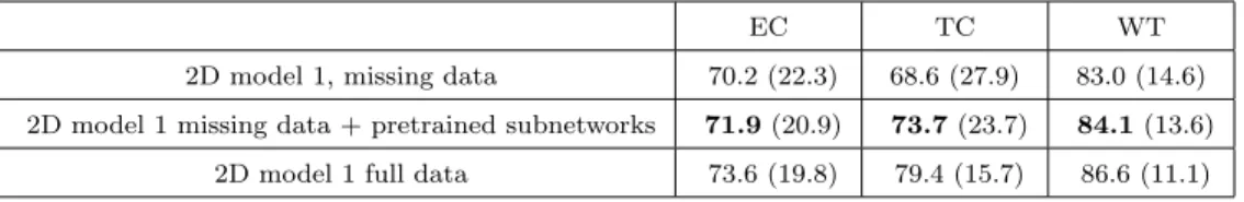
We test our 2D model with modality-specific subnetworks in the context of missing MR sequences in the training database. In this setting, we suppose that the four MR sequences are available only for 20% of patients and that for the remaining patients, one MR sequence out of the four is missing. More precisely, we randomly split the training set of 235 patients in five equal subsets (47 patients in each) and we consider that only the first subset contains all the four MR sequences whereas the four other subsets exclusively miss one MR sequence (T1, T1c, T2 or T2-FLAIR). We previously noted that modality-specific subnetworks can be trained independently: in this case, a subnetwork specific to a given MR sequence can be trained on 80% of the training database (on all training images except the ones for which the MR sequence is missing). The goal of the experiment is to test if the training of these subnetworks improves the segmentation performance in practice. We first evaluate the performance obtained by 2D model 1 (version CNN-2DAxl) trained only on the training subset containing all MR sequences (47 patients). Then we evaluate the performance obtained when the subnetworks are pretrained, each of them using 80% of the training database.
The results are reported in Table 1. Pretraining of the modality-specific subnetworks improved the segmentation performance on the test set for all tumor subregions. Even if the multiclass segmentation problem is very diffi-cult for a small network using only one MR sequence, this pretraining forces
Table 1: Mean Dice scores on the test dataset (50 patients) in the context of misssing MR sequences in the training database. EC, TC and WT refer respectively to ’Enhancing Core’, ’Tumor Core’ and ’Whole Tumor’ regions. The numbers in brackets denote standard deviations.
EC TC WT
2D model 1, missing data 70.2 (22.3) 68.6 (27.9) 83.0 (14.6) 2D model 1 missing data + pretrained subnetworks 71.9 (20.9) 73.7 (23.7) 84.1 (13.6)
the subnetwork to learn the most relevant features, which will then be used by the main part of the network, trained on the subset of training cases for which all MR sequences are available. The improvement was found statisti-cally significant (p-value < 0.05) for all the three tumor subregions (Table 5).
3.4. Using long-range 2D context
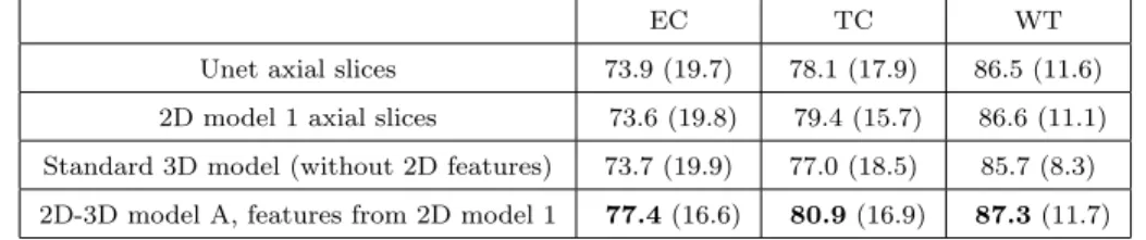
We perform a series of experiments to analyze the effects of using features learned by 2D networks as an additional input to 3D networks. In the first step, 2D model 1 is trained separately on axial, coronal and sagittal slices and the standard 3D model is trained on 70x70x70 patches. Then we extract the features produced by the 2D model for all images of the training database and we train the same 3D model on 70x70x70 patches using these extracted features (Fig. 9) as an additional input (2D-3D model A specified on Fig. 4). The experiment is performed on two datasets: the test dataset of 50 patients (networks trained on the remaining 235 patients) and the Validation dataset of BRATS 2017 (networks trained on 285 patients). The results on the two datasets are reported respectively in Table 2 and Table 3. Further experi-ments, involving varying 2D and 3D architectures are presented in section 3.5. Qualitative analysis is performed on the first dataset, for which the ground truth segmentation is provided. For comparison, we also display the scores obtained by U-net processing axial slices, using our implementation (with batch-normalization).
On the two datasets and for all tumor subregions, our 2D-3D model ob-tained a better performance than the standard 3D CNN (without the use of 2D features) and than 2D model 1 from which the features were extracted (Table 2 and Table 3). The qualitative analysis (Fig. 10) of outputs of 2D networks highlights two main problems of 2D approaches. First, as expected, the produced segmentations show discontinuities which appear as patterns parallel to the planes of processing. The second problem are false positives
Table 2: Mean Dice scores on the test dataset (50 patients). The numbers in brackets denote standard deviations.
EC TC WT
Unet axial slices 73.9 (19.7) 78.1 (17.9) 86.5 (11.6) 2D model 1 axial slices 73.6 (19.8) 79.4 (15.7) 86.6 (11.1) Standard 3D model (without 2D features) 73.7 (19.9) 77.0 (18.5) 85.7 (8.3) 2D-3D model A, features from 2D model 1 77.4 (16.6) 80.9 (16.9) 87.3 (11.7)
Figure 9: 2D features computed for three different patients from the test set. These features correspond to unnormalized outputs of the final convolutional layers of three versions of a 2D model (CNN-2DAxl, CNN-2DSag, CNN-2DCor). The values of these features are used as an additional input to a 3D CNN. Each feature highlights one of the tumor classes (columns 3-6) and encodes a rich information extracted from a long-range 2D context within an axial, sagittal or coronal plane (rows 1-3). Each row displays a different case from the test set (unseen by the network during the training).
in the slices at the borders of the brain and containing artefacts of skull-stripping. Segmentations produced by the standard 3D model are more spa-tially consistent but the network suffers from a limited input information from distant voxels. The use of learned features as an additional input to the network gives a considerable advantage by providing rich information extracted from distant points. The difference of performance is particulary
Table 3: Mean Dice scores on the Validation dataset of BRATS 2017 (46 patients).
EC TC WT
Unet axial slices 71.4 (27.4) 76.6 (22.4) 87.7 (10.6) 2D model 1 axial slices 71.1 (28.8) 78.4 (21.3) 88.6 (8.7) Standard 3D model (without 2D features) 68.7 (30.0) 74.2 (23.7) 85.4 (10.9) 2D-3D model A, features from 2D model 1 76.7 (27.6) 79.5 (21.3) 89.3 (8.5)
Figure 10: Examples of segmentations obtained with models using a different spatial context. Each row represents a different patient from the local test dataset (images unseen during the training). From left to right: MRI T2, ’2D model 1’ processing the image by axial slices, standard 3D model (without 2D features), ’2D-3D model A’ using the features produced by ’2D model 1’, ground truth segmentation. Orange, blue and green zones represent respectively edema, contrast-enhancing core and non-enhancing core.
Figure 11: Results obtained by the 2D-3D model, displayed for each available MR se-quence. While both T2 and T2-FLAIR higlight the edema, T2-FLAIR allows for distin-guishing it from the cerebrospinal fluid. T1 with injection of a gadolinium-based contrast product highlights the degradation of the blood-brain barrier induced by the tumor.
of our 2D-3D approach compared to the standard 3D CNN (without the use of 2D features) were found statistically significant (p-value < 0.05) in all cases except the ’whole tumor’ region in the first dataset (Table 5).
3.5. Varying network architectures and combining segmentations
We perform experiments with varying architectures of 2D and 2D-3D models. The first objective is to test if the use of 2D features provides an improvement when different 2D and 2D-3D architectures are used. The sec-ond objective is to test our decision process combining different multiclass segmentations. The third goal is to compare performances obtained by differ-ent models. The experimdiffer-ents are performed on the Validation set of BRATS 2017, the performance is evaluated by the public benchmark of the challenge.
Figure 12: Architectures of complementary networks used in our experiments.
In our experiments we use two architectures of our 2D model and three architectures of the 2D-3D model. The main difference between the two 2D networks used in experiments is the architecture of subnetworks processing the input MR sequences. In the first 2D model, the subnetworks correspond to reduced versions of U-Net (Fig. 6) whereas in the second model, the sub-networks are composed of three convolutional layers (Fig. 12, top). In the remainder, we refer to these models as ’2D model 1’ and ’2D model 2’. The difference between the two first 2D-3D models is the choice of the layer in which the 2D features are imported: in the first layer of the network (Fig. 4) or before the final sequence of convolutional layers (Fig. 12, bottom left). The third 2D-3D model (Fig. 12, bottom right) is composed of two streams, one processing only the 3D image patch and the other stream taking also the 2D features as input. We refer to these models as 2D-3D model A, 2D-3D model B and 2D-3D model C. Please note that the two first models correspond to a standard 3D model with the only difference of taking an additional input. Each of the 2D-3D models is trained twice using respectively features learned by 2D model 1 or features learned by 2D model 2. We combine the trained 2D-3D models with the voting strategy described in section 2.4. As we observe that 2D model 1 performs better than 2D model 2, we consider two ensembles: combination of all trained 2D-3D models and combination of three models using features from 2D model 1. We use the following thresholds for merging (defined in section 2.4): Ttumor = 0.4, Tcore = 0.3, Tenhancing =
Table 4: Mean Dice scores on the Validation dataset of BRATS 2017 (46 patients).
EC TC WT 2D model 1 axial slices 71.1 78.4 88.6 2D model 2 axial slices 68.0 78.3 88.1 Standard 3D model (without 2D features) 68.7 74.2 85.4 * 2D-3D model A, features from 2D model 1 76.7 79.5 89.3 * 2D-3D model B, features from 2D model 1 76.6 79.1 89.1 * 2D-3D model C, features from 2D model 1 76.9 78.3 89.4 * 2D-3D model A, features from 2D model 2 73.4 79.5 89.7 * 2D-3D model B, features from 2D model 2 74.1 79.4 89.5 * 2D-3D model C, features from 2D model 2 74.3 79.4 89.6 Combination of models A-C features from model 1 76.7 79.6 89.4 Combination of all models * (final segmentation) 77.2 80.8 90.0
Table 5: p-values of the t-tests (in bold: statistically significant results, with p < 0.05) of the improvement provided by the different components of our method. To lighten the notations, ’2D’ refers to ’2D model 1 axial slices’ and ’2D-3D’ refers to ’2D-3D model A, features from 2D model 1’. ’Combination of 2D-3D’ refers to the result obtained by merging 6 models with our hierarchical decision process.
EC TC WT
2D vs 2D with pretrained subnetworks, missing data 0.0054 0.0003 0.0074 Standard 3D vs 2D-3D, dataset 1 0.0082 0.0016 0.0729 Standard 3D vs 2D-3D, dataset 2 0.0077 0.0005 <0.0001
2D-3D vs combination of 2D-3D 0.1058 0.0138 0.0496
0.4.
The results are reported in Table 4. In all experiments, the 2D-3D models obtain better performances than their standard 3D counterparts and than 2D networks from which the features were extracted. The merging of seg-mentations with our decision rule further improves the performance. For all tumor subregions, the ensemble of 6 models (the last row of Table 4) out-performs each of the individual models. The improvement over the main 2D-3D model (2D-3D model A with features from 2D model 1) was found statistically significant (p-value < 0.05) for ’whole tumor’ and ’tumor core’ subregions, as reported in the last row of Table 5. While the three 2D-3D architectures yield similar performances, 2D model 1 (subnetworks similar to
U-net) performs better than 2D model 2 for all three tumor regions. How-ever, the 2D-3D models trained with the features from 2D model 2 are useful for the merging of segmentations: the ensemble of all models yields better performances than the ensemble of three models (two last rows of Table 4).
3.6. Comparison to the state of the art
We have evaluated our segmentation performance on the public bench-mark of the challenge to compare our results with few dozens of teams from renowned research institutions worldwide. Our method compares favorably with competing methods of BRATS 2017 (Table 6): among 55 teams which evaluated their methods on all test patients of the Validation set, we obtain top-3 performance for ’core’ and ’enhancing core’ tumor subregions. We ob-tain mean Dice score of 0.9 for the ’whole tumor’ region, which is almost equal to the one obtained by the best scoring team (0.905).
Table 6: Mean Dice scores of the 10 best scoring teams on the validation leaderboard of BRATS 2017 (state of January 22, 2018)
EC TC WT Rank EC Rank TC Rank WT Average rank UCL-TIG 78.6 83.8 90.5 1 / 55 1 1 1.0 MIC DKFZ 77.6 81.9 90.3 2 / 55 2 2 2.0 inpm (our method) 77.2 80.8 90.0 3 / 55 3 7 4.3 UCLM UBERN 74.9 79.1 90.1 9 / 55 6 3 6.0 biomedia1 73.8 79.7 90.1 12 / 55 5 5 7.3 stryker 75.5 78.3 90.1 6 / 55 10 6 7.3 xfeng 75.1 79.9 89.2 8 / 55 4 11 7.7 Zhouch 75.4 77.8 90.1 7 / 55 12 4 7.7 tkuan 76.5 78.2 88.9 4 / 55 11 13 9.3 Zhao 75.9 78.9 87.2 5 / 55 7 16 9.3
The winning method of UCL-TIG [33] proposes to sequentially use three 3D CNNs in order to progressively determine the tumor subclass. Each of the networks performs a binary segmentation (tumor/not tumor, core/edema, enhancing core/non-enhancing core) and was designed for one tumor subre-gion of BRATS. A common point with our method is the hierarchical process, however in our method all models perform multiclass segmentation. The method of the team MIC DKFZ, according to [34], is based on an optimized version of 3D U-net and an extensive use of data augmentation.
Table 7: Distribution of Dice scores (final result). The numbers in brackets denote stan-dard deviations. EC TC WT Mean 77.2 (24.4) 80.8 (18.9) 90.0 (8.1) Median 85.4 88.3 91.8 Quantile 25 % 76.9 75.0 89.6 Quantile 75 % 90.0 93.5 94.5
The leaderboard of BRATS 2017 only shows mean performances obtained by participating teams. However, the benchmark individually provides de-tailed scores and complementary statistics, in particular quartiles and stan-dard deviations reported in Table 7. Our method yields promising results with median Dice score of 0.918 for the whole tumor, 0.883 for the tumor core and 0.854 for the enhancing core. While the Dice scores for the whole tumor region are rather stable (generally between 0.89 and 0.95), we observe a high variability of the scores obtained for the tumor subregions. In partic-ular the obtained median Dices are much higher than the means, due to the sensitivity of Dice score to outliers.
4. Discussion and conclusion
In this paper we presented a deep learning system for multiclass segmen-tation of tumors in multisequence MR scans. The goal of our work was to propose elements to improve performance, robustness and applicability of commonly used CNN-based systems. In particular, we proposed a new methodology to capture a long-range 3D context with CNNs, we introduced a network architecture with modality-specific subnetworks and we proposed a voting strategy to merge multiclass segmentations produced by different models.
First, we proposed to use features learned by 2D CNNs (capturing a long-range 2D context in three orthogonal directions) as an additional input to a 3D CNN. Our approach combines the strengths of 2D and 3D CNNs and was designed to capture a very large spatial context while being efficient in terms of computations and memory load. Our experiments showed that this hybrid 2D-3D model obtains better performances than both the standard 3D approach (considering only the intensities of voxels of a subvolume) and than the 2D models which produced the features. Even if the use of the additional
input implies supplementary reading operations, the simple importation of few features to a CNN does not considerably increase the number of compu-tations and the memory load. In fact, in typical CNNs performing hundreds of convolutions, max-poolings and upsamplings, the data layer represents typically a very small part of the memory load of the network. One solution to limit the reading operations could be to read downsampled versions of fea-tures or to design a 2D-3D architecture in which the feafea-tures are imported in a part of the network where the feature maps are relatively small.
The improvement provided by the 2D-3D approach has the cost of in-creasing the complexity of the method compared to a pure 3D approach as it requires a two-step processing (first 2D, then 3D). However, its implementa-tion is rather simple as the only supplementary element to implement is the extraction of 2D features, i.e. computation of outputs of trained 2D networks (with a deep learning software such as TensorFlow) and saving the obtained tensors in files. In the 3D part, the extracted features are then simply read as additional channels of the input image.
Despite the important recent progress of GPUs, pure 3D approaches may be easily limited by their computational requirements when the segmenta-tion problem involves an analysis of a very large spatial 3D context. In fact, Convolutional Neural Networks require an important amount of GPU mem-ory and a high computational power as they perform thousands of costly operations on images (convolutions, max-poolings, upsamplings). The main advantage of our 2D-3D approach is to considerably increase the size of the receptive field of the model while being efficient in terms of the computational load. The use of our 2D-3D model may therefore be particularly relevant in the case of very large 3D scans.
Second, we proposed a novel approach to process different MR sequences, using an architecture with modality-specific subnetworks. Such design has the considerable advantage of offering a possibility to train one part of the network on databases containing images with missing MR sequences. In our experiments, training of modality-specific subnetworks improved the segmen-tation performance in the setting with missing MR sequences in the training database. Moreover, the fact that our 2D model obtained promising seg-mentation performance is particularly encouraging given that 2D networks are easier to apply for the clinical use where images have a variable number of acquired slices. Our approach can be easily used with any deep learning software (e.g. Keras). In the case of databases with missing MR sequences, the user only has to perform a training of a subnetwork (on images for which
the given MR sequence is provided) and then read the learned parameters for the training of the main part of the network (on images for which all MR sequences are available).
In order to be less prone to limitations of particular choices of neural network architectures, we proposed to merge outputs of several models by a voxelwise voting strategy taking into account the semantics of labels.
In constrast to most methods, we do not apply any postprocessing on the produced segmentations.
Our methodological contributions can be easily included separately or jointly into a CNN-based system to solve specific segmentation problems. The implementation of our method will be made publicly available on https: //github.com/PawelMlynarski.
Acknowledgements
Pawel Mlynarski is funded by the Microsoft Research-INRIA Joint Center, France. This work was supported by the Inria Sophia Antipolis - M´editerran´ee, ”NEF” computation cluster.
References
[1] M. L. Goodenberger, R. B. Jenkins, Genetics of adult glioma, Cancer genetics 205 (2012) 613–621.
[2] S. Bauer, R. Wiest, L.-P. Nolte, M. Reyes, A survey of mri-based medical image analysis for brain tumor studies, Physics in medicine and biology 58 (2013) R97.
[3] R. J. Gillies, P. E. Kinahan, H. Hricak, Radiomics: images are more than pictures, they are data, Radiology 278 (2015) 563–577.
[4] B. H. Menze, A. Jakab, S. Bauer, J. Kalpathy-Cramer, K. Farahani, J. Kirby, Y. Burren, N. Porz, J. Slotboom, R. Wiest, et al., The multi-modal brain tumor image segmentation benchmark (brats), IEEE trans-actions on medical imaging 34 (2015) 1993–2024.
[5] S. Bakas, H. Akbari, A. Sotiras, M. Bilello, M. Rozycki, J. S. Kirby, J. B. Freymann, K. Farahani, C. Davatzikos, Advancing the cancer genome atlas glioma mri collections with expert segmentation labels and radiomic features, Scientific data 4 (2017) 170117.
[6] M. Prastawa, E. Bullitt, S. Ho, G. Gerig, A brain tumor segmentation framework based on outlier detection, Medical image analysis 8 (2004) 275–283.
[7] A. Gooya, K. M. Pohl, M. Bilello, L. Cirillo, G. Biros, E. R. Melhem, C. Davatzikos, Glistr: glioma image segmentation and registration, IEEE transactions on medical imaging 31 (2012) 1941–1954.
[8] D. Kwon, R. T. Shinohara, H. Akbari, C. Davatzikos, Combining gen-erative models for multifocal glioma segmentation and registration, in: International Conference on Medical Image Computing and Computer-Assisted Intervention, Springer, 2014, pp. 763–770.
[9] N. Cordier, H. Delingette, N. Ayache, A patch-based approach for the segmentation of pathologies: Application to glioma labelling, IEEE transactions on medical imaging 35 (2016) 1066–1076.
[10] S. Bauer, L.-P. Nolte, M. Reyes, Fully automatic segmentation of brain tumor images using support vector machine classification in combination with hierarchical conditional random field regularization, in: Interna-tional Conference on Medical Image Computing and Computer-Assisted Intervention, Springer, 2011, pp. 354–361.
[11] C.-H. Lee, M. Schmidt, A. Murtha, A. Bistritz, J. Sander, R. Greiner, Segmenting brain tumors with conditional random fields and support vector machines, in: International Workshop on Computer Vision for Biomedical Image Applications, Springer, 2005, pp. 469–478.
[12] T. K. Ho, Random decision forests, in: Document Analysis and Recog-nition, 1995., Proceedings of the Third International Conference on, volume 1, IEEE, 1995, pp. 278–282.
[13] D. Zikic, B. Glocker, E. Konukoglu, A. Criminisi, C. Demiralp, J. Shot-ton, O. Thomas, T. Das, R. Jena, S. Price, Decision forests for tissue-specific segmentation of high-grade gliomas in multi-channel mr, in: International Conference on Medical Image Computing and Computer-Assisted Intervention, Springer, 2012, pp. 369–376.
[14] E. Geremia, B. H. Menze, N. Ayache, et al., Spatial decision forests for glioma segmentation in multi-channel mr images, MICCAI Challenge on Multimodal Brain Tumor Segmentation 34 (2012).
[15] L. Le Folgoc, A. V. Nori, S. Ancha, A. Criminisi, Lifted auto-context forests for brain tumour segmentation, in: International Workshop on Brainlesion: Glioma, Multiple Sclerosis, Stroke and Traumatic Brain Injuries, Springer, 2016, pp. 171–183.
[16] S. Bauer, T. Fejes, J. Slotboom, R. Wiest, L.-P. Nolte, M. Reyes, Seg-mentation of brain tumor images based on integrated hierarchical classi-fication and regularization, in: MICCAI BraTS Workshop. Nice: Miccai Society, 2012.
[17] N. J. Tustison, K. Shrinidhi, M. Wintermark, C. R. Durst, B. M. Kan-del, J. C. Gee, M. C. Grossman, B. B. Avants, Optimal symmetric multimodal templates and concatenated random forests for supervised brain tumor segmentation (simplified) with antsr, Neuroinformatics 13 (2015) 209–225.
[18] Y. LeCun, Y. Bengio, et al., Convolutional networks for images, speech, and time series, The handbook of brain theory and neural networks 3361 (1995) 1995.
[19] K. He, X. Zhang, S. Ren, J. Sun, Deep residual learning for image recognition, in: Proceedings of the IEEE conference on computer vision and pattern recognition, 2016, pp. 770–778.
[20] A. Krizhevsky, I. Sutskever, G. E. Hinton, Imagenet classification with deep convolutional neural networks, in: Advances in neural information processing systems, 2012, pp. 1097–1105.
[21] K. Simonyan, A. Zisserman, Very deep convolutional networks for large-scale image recognition, arXiv preprint arXiv:1409.1556 (2014).
[22] P. Sermanet, D. Eigen, X. Zhang, M. Mathieu, R. Fergus, Y. LeCun, Overfeat: Integrated recognition, localization and detection using con-volutional networks, arXiv preprint arXiv:1312.6229 (2013).
[23] J. Long, E. Shelhamer, T. Darrell, Fully convolutional networks for semantic segmentation, in: Proceedings of the IEEE Conference on Computer Vision and Pattern Recognition, 2015, pp. 3431–3440.
[24] L.-C. Chen, G. Papandreou, I. Kokkinos, K. Murphy, A. L. Yuille, Se-mantic image segmentation with deep convolutional nets and fully con-nected crfs, arXiv preprint arXiv:1412.7062 (2014).
[25] S. Pereira, A. Pinto, V. Alves, C. A. Silva, Deep convolutional neural networks for the segmentation of gliomas in multi-sequence mri, in: In-ternational Workshop on Brainlesion: Glioma, Multiple Sclerosis, Stroke and Traumatic Brain Injuries, Springer, 2015, pp. 131–143.
[26] K. Kamnitsas, C. Ledig, V. F. Newcombe, J. P. Simpson, A. D. Kane, D. K. Menon, D. Rueckert, B. Glocker, Efficient multi-scale 3d cnn with fully connected crf for accurate brain lesion segmentation, arXiv preprint arXiv:1603.05959 (2016).
[27] O. Ronneberger, P. Fischer, T. Brox, U-net: Convolutional networks for biomedical image segmentation, in: International Conference on Medical Image Computing and Computer-Assisted Intervention, Springer, 2015, pp. 234–241.
[28] M. Havaei, A. Davy, D. Warde-Farley, A. Biard, A. Courville, Y. Bengio, C. Pal, P.-M. Jodoin, H. Larochelle, Brain tumor segmentation with deep neural networks, Medical image analysis 35 (2017) 18–31.
[29] Q. Zheng, H. Delingette, N. Duchateau, N. Ayache, 3d consistent & robust segmentation of cardiac images by deep learning with spatial propagation, IEEE Transactions on Medical Imaging (2018).
[30] Q. Dou, L. Yu, H. Chen, Y. Jin, X. Yang, J. Qin, P.-A. Heng, 3d deeply supervised network for automated segmentation of volumetric medical images, Medical Image Analysis (2017).
[31] ¨O. C¸ i¸cek, A. Abdulkadir, S. S. Lienkamp, T. Brox, O. Ronneberger, 3d u-net: Learning dense volumetric segmentation from sparse annotation, arXiv preprint arXiv:1606.06650 (2016).
[32] K. Kamnitsas, W. Bai, E. Ferrante, S. McDonagh, M. Sinclair, N. Pawlowski, M. Rajchl, M. Lee, B. Kainz, D. Rueckert, et al., En-sembles of multiple models and architectures for robust brain tumour segmentation, arXiv preprint arXiv:1711.01468 (2017).
[33] G. Wang, W. Li, S. Ourselin, T. Vercauteren, Automatic brain tumor segmentation using cascaded anisotropic convolutional neural networks, arXiv preprint arXiv:1709.00382 (2017).
[34] F. Isensee, P. Kickingereder, W. Wick, M. Bendszus, K. H. Maier-Hein, Brain tumor segmentation and radiomics survival prediction: Contri-bution to the brats 2017 challenge, 2017 International MICCAI BraTS Challenge (2017).
[35] J. Lafferty, A. McCallum, F. C. Pereira, Conditional random fields: Probabilistic models for segmenting and labeling sequence data (2001). [36] J. Serra, P. Soille, Mathematical morphology and its applications to image processing, volume 2, Springer Science & Business Media, 2012. [37] S. E. Dreyfus, Artificial neural networks, back propagation, and the
kelley-bryson gradient procedure, Journal of Guidance, Control, and Dynamics 13 (1990) 926–928.
[38] F. Ciompi, K. Chung, S. J. Van Riel, A. A. A. Setio, P. K. Gerke, C. Ja-cobs, E. T. Scholten, C. Schaefer-Prokop, M. M. Wille, A. Marchian`o, et al., Towards automatic pulmonary nodule management in lung cancer screening with deep learning, Scientific Reports 7 (2017).
[39] J. Bergstra, O. Breuleux, F. Bastien, P. Lamblin, R. Pascanu, G. Des-jardins, J. Turian, D. Warde-Farley, Y. Bengio, Theano: A cpu and gpu math compiler in python, in: Proc. 9th Python in Science Conf, 2010, pp. 1–7.
[40] M. Abadi, A. Agarwal, P. Barham, E. Brevdo, Z. Chen, C. Citro, G. S. Corrado, A. Davis, J. Dean, M. Devin, et al., Tensorflow: Large-scale machine learning on heterogeneous distributed systems, arXiv preprint arXiv:1603.04467 (2016).
[41] D. E. Rumelhart, G. E. Hinton, R. J. Williams, Learning representations by back-propagating errors, Cognitive modeling 5 (1988) 1.
[42] L. G. Ny´ul, J. K. Udupa, X. Zhang, New variants of a method of mri scale standardization, IEEE transactions on medical imaging 19 (2000) 143–150.
[43] J. G. Sled, A. P. Zijdenbos, A. C. Evans, A nonparametric method for automatic correction of intensity nonuniformity in mri data, IEEE transactions on medical imaging 17 (1998) 87–97.
[44] S. Ioffe, C. Szegedy, Batch normalization: Accelerating deep net-work training by reducing internal covariate shift, arXiv preprint arXiv:1502.03167 (2015).