HAL Id: hal-02105151
https://hal.archives-ouvertes.fr/hal-02105151
Submitted on 16 Sep 2020
HAL is a multi-disciplinary open access
archive for the deposit and dissemination of
sci-entific research documents, whether they are
pub-lished or not. The documents may come from
teaching and research institutions in France or
abroad, or from public or private research centers.
L’archive ouverte pluridisciplinaire HAL, est
destinée au dépôt et à la diffusion de documents
scientifiques de niveau recherche, publiés ou non,
émanant des établissements d’enseignement et de
recherche français ou étrangers, des laboratoires
publics ou privés.
Non-uniform seasonal warming regulates vegetation
greening and atmospheric CO 2 amplification over
northern lands
Zhao Li, Jianyang Xia, Anders Ahlström, Annette Rinke, Charles Koven,
Daniel J Hayes, Duoying Ji, Geli Zhang, Gerhard Krinner, Guangsheng Chen,
et al.
To cite this version:
Zhao Li, Jianyang Xia, Anders Ahlström, Annette Rinke, Charles Koven, et al.. Non-uniform seasonal
warming regulates vegetation greening and atmospheric CO 2 amplification over northern lands.
Envi-ronmental Research Letters, IOP Publishing, 2018, 13 (12), pp.124008. �10.1088/1748-9326/aae9ad�.
�hal-02105151�
LETTER • OPEN ACCESS
Non-uniform seasonal warming regulates vegetation greening and
atmospheric CO
2
amplification over northern lands
To cite this article: Zhao Li et al 2018 Environ. Res. Lett. 13 124008
View the article online for updates and enhancements.
Environ. Res. Lett. 13(2018) 124008 https://doi.org/10.1088/1748-9326/aae9ad
LETTER
Non-uniform seasonal warming regulates vegetation greening and
atmospheric CO
2
ampli
fication over northern lands
Zhao Li1,2 , Jianyang Xia1,2,22 , Anders Ahlström3,4 , Annette Rinke5,6 , Charles Koven7 , Daniel J Hayes8 , Duoying Ji5 , Geli Zhang9 , Gerhard Krinner10 , Guangsheng Chen8 , Wanying Cheng1,2 , Jinwei Dong11 , Junyi Liang12, John C Moore5, Lifen Jiang13, Liming Yan1,2, Philippe Ciais14, Shushi Peng14,15,16,17, Ying-Ping Wang18, Xiangming Xiao19,20, Zheng Shi19, A David McGuire21 and Yiqi Luo13
1 Tiantong National Station of Forest Ecosystem and Research Center for Global Change and Ecological Forecasting, School of Ecological
and Environmental Sciences, East China Normal University, Shanghai 200241, People’s Republic of China
2 Institute of Eco-Chongming(IEC), 3663 N. Zhongshan Rd., Shanghai 200062, People’s Republic of China 3 Department of Physical Geography and Ecosystem Science, Lund University, SE 223 62 Lund, Sweden
4 Department of Earth System Science, School of Earth, Energy and Environmental Sciences, Stanford University, 473 Via Ortega, Stanford,
CA 94305, United States of America
5 College of Global Change and Earth System Science, Beijing Normal University, Beijing, People’s Republic of China 6 Alfred Wegener Institute Helmholtz Centre for Polar and Marine Research, Potsdam, Germany
7 Lawrence Berkeley National Laboratory, Berkeley, CA, United States of America
8 School of Forest Resources, University of Maine, Orono, ME 04469, United States of America
9 College of Land Science and Technology, China Agricultural University, Beijing 100193, People’s Republic of China 10 CNRS, Université Grenoble Alpes, IGE, 38000 Grenoble, France
11 Key Laboratory of Land Surface Pattern and Simulation, Institute of Geographic Sciences and Natural Resources Research, Chinese
Academy of Sciences, Beijing 100101, People’s Republic of China
12 Environmental Sciences Division & Climate Change Science Institute, Oak Ridge National Laboratory, Oak Ridge, TN 37830, United
States of America
13 Department of Biological Sciences, Northern Arizona University, Flagstaff, Arizona, United States of America
14 Laboratoire des Sciences du Climat et de l’Environnement, CEA-CNRS-UVSQ, UMR8212, 91191 Gif-sur-Yvette, France 15 CNRS, Laboratoire de Glaciologie et Géophysique de l’Environnement (LGGE), 38041 Grenoble, France
16 College of Urban and Environmental Sciences Peking University, Beijing, People’s Republic of China 17 Université Grenoble Alpes, LGGE, 38041 Grenoble, France
18 CSIRO Oceans and Atmosphere, PMB 1, Aspendale, Victoria 3195, Australia
19 Department of Microbiology and Plant Biology, Center for Spatial Analysis, University of Oklahoma, OK 73019, United States of America 20 School of Life Sciences, Fudan University, Shanghai, 200433, People’s Republic of China
21 Institute of Arctic Biology, University of Alaska Fairbanks, Fairbanks, AK, United States of America 22 Author to whom any correspondence should be addressed.
E-mail:jyxia@des.ecnu.edu.cn
Keywords: slowed down, asymmetric response, non-uniform seasonal warming, atmospheric CO2amplitude
Supplementary material for this article is availableonline
Abstract
The enhanced vegetation growth by climate warming plays a pivotal role in amplifying the seasonal cycle of
atmospheric CO
2at northern lands
(>50° N) since 1960s. However, the correlation between vegetation
growth, temperature and seasonal amplitude of atmospheric CO
2concentration have become elusive with
the slowed increasing trend of vegetation growth and weakened temperature control on CO
2uptake since
late 1990s. Here, based on in situ atmospheric CO
2concentration records from the Barrow observatory
site, we found a slowdown in the increasing trend of the atmospheric CO
2amplitude from 1990s to
mid-2000s. This phenomenon was associated with the paused decrease in the minimum CO
2concentration
([CO
2]
min), which was significantly correlated with the slowdown of vegetation greening and
growing-season length extension. We then showed that both the vegetation greenness and growing-growing-season length
were positively correlated with spring but not autumn temperature over the northern lands. Furthermore,
such asymmetric dependences of vegetation growth upon spring and autumn temperature cannot be
captured by the state-of-art terrestrial biosphere models. These
findings indicate that the responses of
vegetation growth to spring and autumn warming are asymmetric, and highlight the need of improving
autumn phenology in the models for predicting seasonal cycle of atmospheric CO
2concentration.
OPEN ACCESS
RECEIVED
17 April 2018
REVISED
15 October 2018
ACCEPTED FOR PUBLICATION
19 October 2018
PUBLISHED
27 November 2018
Original content from this work may be used under
the terms of theCreative
Commons Attribution 3.0 licence.
Any further distribution of this work must maintain attribution to the author(s) and the title of the work, journal citation and DOI.
1. Introduction
Temporal dynamics of atmospheric CO2
concentra-tion, climate and terrestrial carbon (C) cycle are strongly linked in the present(Schneising et al2014) and past (Montañez et al 2016) Earth systems. For example, the recent inter-annual variability of atmo-spheric CO2growth rate is largely caused by
fluctua-tions in terrestrial CO2 uptake (Myneni et al1997,
Keenan et al 2016), which is mainly driven by variations in climate(Poulter et al2014, Ahlström et al 2015, Jung et al 2017). On the decadal scale, an increasing amplitude of the atmospheric CO2seasonal
cycle at northern high latitudes has been observed since 1960s(Bacastow et al1985, Keeling et al1996, Randerson et al1997, Graven et al2013), e.g. about 0.53% yr−1 at the Point Barrow (BRW) during 1971–2011 (Forkel et al 2016). Although the major contributors to such trend of seasonal atmospheric CO2amplitude are still in debate(Gray et al2014, Zeng
et al2014, Ito et al2016, Wenzel et al2016, Piao et al 2017a), the associated increases in mean annual temperature(MAT) and vegetation growth has been recognized as one important driver(Forkel et al2016, Gonsamo et al2017, Piao et al2017a, Yuan et al2018). Recently, non-uniform warming trends among sea-sons have been detected over the northern lands(Xu et al2013, Xia et al2014). Given that climate warming in different seasons would influence vegetation growth differently(Xu et al2013, Xia et al2014, Cai et al2016), the role of seasonal non-uniform warming in affecting the vegetation growth as well as the recent changes of the atmospheric CO2amplitude remains unclear.
Some recent evidence has implied weakening cor-relations of MAT with vegetation growth and atmo-spheric CO2concentration in the past three decades.
First, the MAT across the northern high latitudes has kept rising whereas vegetation greenness has begun to decline since late 1990s(Bhatt et al2013, Jeong et al 2013). Second, the advanced spring phenology in response to climate warming has been reported to diminish at northern high latitudes over the last two decades (Fu et al 2015, Wang et al2015). Third, a weakening inter-annual correlation of temperature with vegetation greenness(Piao et al2014) or spring ecosystem CO2 uptake (Piao et al 2017b) has been
detected at northern latitudes during recent years. In northern temperate ecosystems, a negative correlation between the atmospheric CO2amplitude and
temper-ature anomalies during 2000s has been found through the analysis of space-borne atmospheric CO2
mea-surements(Schneising et al2014). Thus, it is impor-tant to examine how the temperature changes in different seasons have contributed to such weakening correlations of MAT with vegetation growth and sea-sonal CO2amplitude in recent years.
In this study, we investigated the relationships between changes in the seasonal CO2amplitude,
vege-tation greenness and seasonal air temperature in northern lands(>50° N) during the last three decades. The analyses were based on long-term monitoring records of atmospheric CO2, global gridded climate
datasets, and satellite-derived Normalized Difference Vegetation Index(NDVI). We also examined the rela-tionships between temperature and gross primary productivity(GPP) in five terrestrial biosphere models (TBMs), which have been commonly incorporated into Earth system models for future projections of cli-mate and atmospheric changes.
2. Data and methods
2.1. Atmospheric CO2measurements
There are 19 CO2measurement sites in the NOAA’s
Global Greenhouse Gas Reference Network(https:// esrl.noaa.gov/gmd/ccgg/ggrn.php) and 3 sites in Scripps CO2 program (http://scrippsco2.ucsd.edu/ data/atmospheric_co2/sampling_stations) located at lands over 50° N. Among these sites, only the Barrow (BRW) observatory site recorded the atmospheric CO2
concentration (i.e. [CO2]) continuously during
1982–2010. Thus, in this study, the in situ long-term CO2measurements from BRW were regarded as the
homogeneous CO2 concentration in northern lands
(>50° N). The seasonal curve of this [CO2] record was
shown infigure S1 (available online atstacks.iop.org/ ERL/13/124008/mmedia).
The in situ [CO2] observations at the BRW site
were collected hourly. The daily and monthly data provided by NOAA were averaged from the hourly observations. This study used the monthly data to derive the CO2amplitude. The anomalies of monthly
[CO2] (i.e. monthly [CO2] − yearly mean [CO2]) were
first calculated and then were used to derive the max-imum (i.e. [CO2]max) and minimum (i.e. [CO2]min)
monthly[CO2] in each year. The difference between
[CO2]maxand[CO2]minwas defined as the CO2
ampl-itude([CO2]amplitude).
To avoid the biases of various processing algo-rithms, we collected the estimates of [CO2]amplitude
from Forkel et al(2016) and the GLOBALVIEW pro-ducts(figure S2). In Forkel et al (2016), the time series of daily[CO2] records were first fitted with polynomial
and harmonics functions and then de-trended with the Fast Fourier Transformation method (Thoning et al1989, Thoning et al2015). In each calendar year, the[CO2]amplitudewas calculated as the peak-to-trough
difference of the de-trended seasonal cycle. The data in the GLOBALVIEW-CO2 product has already been
smoothed, interpolated and extrapolated(Masane and Tans 1955). GLOBALVIEW-CO2 provides
the difference between the maximum and minimum weekly CO2data in each calendar year. According to
the Theil–Sen analysis, the long-term trends of [CO2]amplitudewere consistent among these processing
methods(figure S2). 2.2. Temperature analysis
The temperature trends were analyzed based on the latest version of the CRU temperature data(CRU TS4.0). It is gridded with a spatial resolution of 0.5°×0.5° at a monthly time step. This product is gridded using the Angular-distance weighting interpolation (Harris and Jones2017) based on the observations collected from 2600 stations worldwide(Harris et al2014). The CRU climate products have been widely used for phenology analysis and for driving different types of ecosystem models(Koven et al2011, Fu et al2014, Xia et al2017). In this study, seasonal temperature was averaged from monthly temperature following the definition of four seasons: Spring, March–May; Summer, June–August; Autumn, September–November; Winter, December– February. Besides, MAT of a given year was defined as the average of the monthly temperature from January to December. The Theil–Sen estimator and Mann-Kendall trend test were applied in detecting the temporal trends of the seasonal temperature (see more details in section2.6).
2.3. Satellite derived NDVI
The normalized difference vegetation index(NDVI) is widely used as an indicator for vegetation productivity (Myneni et al1997, Zhou et al2001). It is calculated as the normalized ratio between near infrared and red reflectance bands (Tucker 1979, Tucker et al2005). The NDVI used in this study is from the Advanced Very High Resolution Radiometer sensors, which has the longest record of continuous satellite data since 1981. Here, we used the newest version of GIMMS NDVI dataset(NDVI3g) (Tucker et al2005, Pinzon and Tucker 2014). It is a global product at spatial resolution of∼8×8 km and temporal resolution of 15 d. The NDVI3g has been widely used for analyzing vegetation changes in recent years(Tucker et al2005, Peng et al2013, Wang et al2014). The maximum value composites method (Holben 1986) was applied to merge segmented data strips to half-monthly values. To lessen the impacts of sparse soils and snows on vegetation, following Zhang et al(2013), the areas with multiyear average NDVI less than 0.1 in the northern lands (>50° N) were removed from the analysis. Moreover, only the half-monthly NDVI from January to September were used to derive the phenology indices (i.e. start and end of growing season length (GSL), see section2.4).
The sum of monthly NDVI from January to Decem-ber in a certain year was regard as the yearly NDVI (Gonsamo et al2016,2017). Note that the illegitimate signals of the half-monthly NDVI data(i.e. NDVI<0.1)
werefiltered. Regional NDVI used in the trend analysis were averaged from the grids of the northern lands (>50° N). Before calculating the sensitivity of NDVI to MAT and the partial correlation between NDVI and sea-sonal temperature(see section2.6), yearly NDVI data were resampled to raster of 0.5°×0.5°, to couple with the CRU temperature data.
2.4. Method of determining GSL
GSL was calculated as the difference between the start (SOS) and end (EOS) of growing season. The SOS and EOS were retrieved from the seasonal NDVI curve in each year based on the NDVI green-up thresholds, which were determined from the rate of seasonal changes in the multiyear mean NDVI (Piao et al 2006,2011, Zhang et al2013). More specifically, there were six steps in the determination of GSL. First, we calculated the seasonal curve of multiyear mean NDVI from 1982 to 2010 for each land grid cell and obtained the changing rate of NDVI(NDVIratio) as:
= + -( ) [ ( ) ( )] [ ( )] / t t t t
NDVI NDVI 1 NDVI
NDVI ,
ratio
where t is time throughout the year with an interval of 15 d. Then, after removing evident noise in the multi-year mean time-series curve of NDVI for each land grid cell, we performed a least-square regression analysis on the curves from January to September and from July to December for determining the NDVI thresholds of SOS and EOS, respectively, with an inverted parabola equation:
= +a a x+a x + ¼ +a x
NDVI 1 2 2 n n,
where x is the Julian days and n is 6. The corresponding NDVI(t) with the maximum or minimum NDVIratio
was used as the NDVI threshold for determining SOS or EOS, respectively. Next, we performed a least-square regression analysis on the NDVI time-series curve in each year for each pixel after removing noise in the two different periods. After that, the SOS and EOS were identified from the fitted NDVI seasonal curves and their NDVI thresholds, by selecting the day when thefitted NDVI curve first reached the NDVI threshold. Finally, the GSL in each year for each land cell was calculated from the difference between EOS and SOS. The method in this study had been validated by ground-based phenological data in Tibetan Plateau (Zhang et al 2013) and has been widely used for detecting phenological changes in various regions (Piao et al2006, Piao et al2011, Zhang et al2013). 2.5. Simulated GPP by TBMs
Outputs of annual GPP from five TBMs which provided all the land cells above the 50° N in the model integration group of the Permafrost Carbon Network (http://permafrostcarbon.org/) were analyzed in this study. Thefive TBMs are UVic (Peter2001, Matthews et al 2004), CoLM (Dai et al 2003, Ji et al 2014), CLM4.5 (Oleson et al 2003), TEM604 (Hayes et al 2011) and ORCHIDEE (Krinner et al2005). Details 3
about these TBMs were listed in table S1. The simulation protocol and model’s driving data have been described in previous studies(Rawlins et al2015, McGuire et al2016, Peng et al2016). A flux-tower-based GPP database was also used in this study. It was up-scaled from FLUXNET observations (44 sites locating in the lands northern 50° N) of carbon dioxide, energy and water fluxes with the machine learning technique of model tree ensembles (MTE, Jung et al2011). The MTE GPP is a global gridded product with a resolution of 0.5°×0.5°. This product has been widely used as benchmarks to evaluate model performance in recent years(Anav et al2013, Tjiputra et al2013, Peng et al2015, Xia et al2017).
2.6. Statistical analyses
We estimated the linear trends of the CO2indices(i.e.
[CO2]amplitude, [CO2]max and [CO2]min), vegetation
and temperature using a non-parametric Theil–Sen estimator over each time period. The significance of the trend was computed by the Mann-Kendall trend test. Comparing with the ordinary least squares estimation, the Theil–Sen estimator and Mann-Ken-dall trend test is less sensitive to outliers(Fernandes and Leblanc 2005, Wang et al 2018). The temporal anomalies were used for the linear-trend analyses. This analysis can provide both trend and its level of significance (i.e. the P value that quantifies the prob-ability of whether the trend is statistically significant from zero) for each period.
The moving-window method was used to detect whether the increasing trends of CO2indices are
per-sistent. Comparing with the piecewise linear fitting method, it less depends on the results of single linear segment and the interval-length(Schleip et al2008). This method has been used in detecting the changes of growing-season length and its response to climate change on various time scales(Rutishauser et al2007, Schleip et al2008, Jeong et al 2011, Fu et al2015). Because the results based the moving-window analysis may be affected by the window-length(Fu et al2015), we repeated the moving-window analyses with ten-, 15- and 20-year lengths.
The temporal trends of MAT(DMAT), the sensitivity
of NDVI to temperature(gNDVI), and the sensitivity of CO2amplitude to temperature(g[CO2 amplitude] ) in the
peri-ods of 1982–2010 and 1993–2007 were calculated in each grid cell. The gNDVIand g[CO]
2 amplitudewere derived from
the slope of linear regressions, representing the changes of NDVI and[CO2]amplitudewith per degree change of
MAT. One-way ANOVA was used to estimate their dif-ferences between 1982–2010 and 1993–2007. All the analyses were applied inR (http://r-project.org/).
Partial correlation analyses were applied to exclude the impacts of the co-varying factors. For example, in calculating the impact of spring temper-ature on SOS, spring precipitation, spring solar radia-tion and last-year’s autumn temperature were set as
the controlling variables. Autumn precipitation, autumn solar radiation and spring temperature were set as the controlling variables to quantify the impact of autumn temperature on EOS. Similar method was used to detect the impact of spring and autumn temp-erature on annual NDVI and modeled GPP by repla-cing the seasonal precipitation and solar radiation with annual values. All the data were aggregated to the 0.5°× 0.5° resolution. The precipitation data were derived from the CRU TS4.0 dataset(Harris et al2014) and the radiation data was from the Terrestrial Hydrology Research Group at Princeton University (Sheffield et al2006).
3. Results and discussion
3.1. The temporal changes of atmospheric CO2
seasonal cycle and vegetation greenness
We first examined the trends of the measured annual CO2 amplitude ([CO2]amplitude) at Point
BRW, Alaska (71°N). The non-parametric Theil– Sen estimator showed that the increasing trends of the [CO2]amplitude at the BRW (0.075 ppm yr−1,
P<0.05; figure 1(a)) were associated with the decreasing[CO2]min(−0.058 ppm yr−1, P<0.05)
rather than the enhancing [CO2]max (0.016 ppm
yr−1, P=0.17) from 1982 to 2010. The ten-year moving windows show that the increasing rates of the CO2 amplitude was slower around 2000
(figure1(a) and table S2). To avoid the biases from different time-intervals for trend estimation, we also detected the trends with 15-year (figure S3) and 20-year (figure S4) moving windows. The results also showed that the trends of[CO2]amplitudefrom
mid-1990 to mid-2000 (e.g. 0.03 ppm yr−1, P=0.55, 1993–2007) (figure S4(a) and table S4) were significantly slower than those during other periods. A recent study which integrated the CO2
records from multiple sites also has showed a stalled trend in the seasonality of atmospheric CO2during
the same period(Yuan et al2018).
A slowdown of vegetation greening since mid-1990s was also observed by our analysis on the dynamics of NDVI(figures1(b) and S5(d)). This finding is consistent with the results from recent analyses on vegetation dynamics over the pan-Arctic tundra(Bhatt et al2013, Jeong et al2013). Both the MTE GPP (figure S5(e)) and the ground-based measurements of growing-season net ecosystem CO2exchange(figure S5(f)), the net
ecosys-tem exchange data were derived from Belshe et al(2013) showed similar trends since 1990s. These lines of evi-dences together suggest that the increasing trend of the growing-season CO2uptake has weakened from 1990s to
mid-2000s in northern ecosystems.
Meanwhile, a weak but significant linear relation-ship between average NDVI over the northern lands (>50° N) and [CO2]minat the BRW site was observed
The synchronous changes of [CO2]amplitude with
[CO2]min (figures S5(a)–(c)) and NDVI (figure 1)
imply that the long-term positive trend of [CO2]amplitude is, at least in part, driven by
photo-synthetic CO2 uptake or vegetation growth (Forkel
et al2016, Wenzel et al2016).
3.2. The asymmetric responses of vegetation growth to spring and autumn warming
An increasing body of research has shown a non-linear response or reduced sensitivity of vegetation growth to rising MAT over high latitudes in recent years(Bhatt et al 2013, Jeong et al2013, Piao et al2014). As shown by figure2, although the MAT increased even faster from mid-1990s to mid-2000s(e.g. 1993–2007) than the whole period of 1982–2010, the sensitivities of [CO2]amplitude
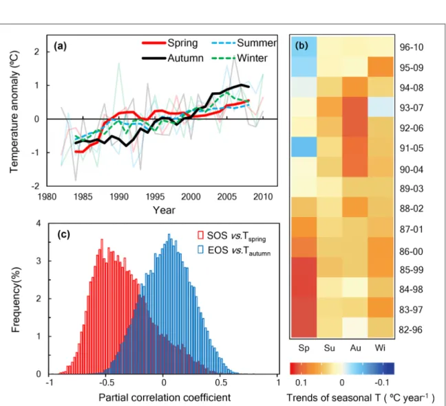
and NDVI to MAT were lower during that period than 1982–2010. Given the fact that temperature in different seasons has non-uniform impacts on vegetation growth (Xia et al 2014), we further analyzed the changes of seasonal temperatures based on the CRU temperature datasets (see methods). As shown by figure 3(b), the fastest warming season was spring during 1985–1999 (+0.12 °C year−1) but then changed to autumn during
mid-1990s to mid-2000s (e.g. +0.11 °C year−1 in
1993–2007, table S4). It indicates that a better under-standing of the relationship between the seasonal temp-erature changes and vegetation growth is needed to explain the slowdown of[CO2]amplitudefrom 1990s to
mid-2000s.
The variation of NVDI during 1982–2010 in north-ern ecosystems depends substantially on the GSL on both grid and regional scales(figures1(b) and S6). Fur-ther partial correlation analysis showed that the SOS (partial r = −0.36) was more dependent on temperature change than the EOS(partial r = 0.018, figures3(c) and S7). During 1982–2010, the SOS was advanced by 2.15 d °C−1with spring warming, whereas warming in autumn
only delayed EOS by 0.80 d°C−1in northern ecosys-tems. As a result, the advancing rate of SOS over the moving 15 years has decreased but the extending rate of EOS was not significantly increased during 1982–2010 (figure S8 and table S5). Meanwhile, the increasieng rate of NDVI until it stalled in mid-1990s is driven by warm-ing-induced increase in spring and early summer NDVI along with the advancement of SOS (figure S8), for which spring warming has stalled after mid-1990s. It has contributed to the decline in the rate of[CO2]amplitude
increase since the mid-1990s. These results together sug-gest that the non-uniform warming between spring and autumn during mid-1990s and mid-2000s(figure3(b))
Figure 1. Changes in temporal trends of CO2amplitude and plant growth(NDVI). The ten-year moving window from 1982 to 2010
shows the changing trends of(a), the peak-to-trough amplitude ([CO2]amplitude) and yearly maximum CO2concentration([CO2]max)
as well as the minimum CO2concentration([CO2]min) at Point Barrow (BRW); (b) NDVI and growing season length (GSL). The
insert in panel(a) shows the long-term trends of [CO2]amplitude(red column, 0.075 ppm yr−1, P<0.01), [CO2]min(green column,
−0.058 ppm yr−1, P<0.01) and [CO
2]max(blue column, 0.016 ppm yr-1, P=0.17) across 1982 to 2010. The insert in panel (b) shows
the correlation between the yearly anomalies of the[CO2]minand NDVI during 1982–2010 (with r=−0.47, P<0.05).
5
Figure 3. Temporal variations of seasonal temperature over northern lands(>50° N). (a) The year-to-year anomalies were shown by the transparent lines and theirfive-year running means were displayed by the solid (spring and autumn) and dashed lines (summer and winter). (b) 15-year moving windows from 1982 to 2010 show the trends of seasonal temperature changes. (c) Frequency histograms of the sensitivity(i.e. the partial correlation coefficient) of SOS to spring temperature change (SOS versus Tspring) and EOS
to autumn temperature change(EOS versus Tautumn) from 1982 to 2010. Note that the negative values of the X-axis represent the
advanced SOS or EOS with temperature increase.
Figure 2.(a) The changes of mean annual temperature, ΔMAT, °C yr−1and the temperature sensitivities of atmospheric CO2seasonal
amplitude.(b) γ[CO2]amplitude, (10 ppm °C
−1) and of the NDVI. (c) γ
NDVI,°C−1during 1982–2010 and 1993–2007.***Significant
could be an important driving factor for the slowdown of expanding GSL, greening vegetation and the decreasing [CO2]min. This can qualitatively explain the pause in the
enhancement of[CO2]amplitude(figure1(a)).
3.3. The response of vegetation productivity to spring and autumn warming in current TBMs We examined whether TBMs that have been focusing on simulation of C dynamics in northern latitudes can adequately represent the differential impacts of spring and autumn warming on vegetation productivity. The ensemble output of GPP fromfive TBMs (CLM4.5, CoLM, ORCHIDEE, TEM6 and UVic; table S1) and a flux-based GPP dataset (MTE) were analyzed (figure4). The dependence of modeled GPP variations on spring-temperature change(with the inter-model mean partial r as 0.57 under the significant level of P<0.05) is comparable with that of the MTE GPP (partial r=0.53, P<0.05) as well as that of NDVI (partial r=0.49, P<0.05; figure4(b) and figure S9). However, the dependences of GPP variations on autumn-temperature change is more positive in the models(inter-model mean partial r=0.31, P < 0.05) than the MTE GPP(partial r=−0.04, P<0.05) and NDVI(partial r=−0.16, P<0.05; figures4(b) and S10). This mismatch between modeling and data-oriented results indicates that the current TBMs over-estimate the positive impact of rising MAT on ecosystem CO2uptake in the autumn.
As the land biogeochemical component in most Earth system models is similar to the TBMs in this study, it is still challenging to accurately simulate the seasonal cycle of atmospheric CO2. Thefindings of
this study suggest that a better representation of the
warming impacts on autumn phenology could par-tially improve the models’ performance. However, the autumn phenology is diversely represented in differ-ent models. For example, leaf senescence in the ORCHIDEE model is simulated as the timing when monthly temperature falls below a given number, which varies with plant function type(Krinner et al 2005). In the TEM, growing season ended when the soil temperature is lower than the frozen point. How-ever, leaf-senescence events are collectively affected by not only temperature but also day length(Ballantyne et al 2017), radiation (Bauerle et al 2012) and even spring phenology(Keenan and Richardson2015, Liu et al2016). In fact, the poor representation of autumn phenology by the models has been raised in some pre-vious studies(Richardson et al2010,2012, Keenan and Richardson 2015). Thus, combining the different types of phenological data(e.g. Richardson et al2018) with better phenology models could be helpful to improve the simulation of the seasonal cycle of atmo-spheric CO2at high latitudes in Earth system models.
3.4. The role of the non-uniform warming in regulating the seasonal atmospheric CO2cycle
This study highlights that the asymmetric responses of vegetation growth to spring and autumn warming is an important driver for the decadal changes in the seasonality of atmospheric CO2. In spring, solar
radiation is not limiting as temperature(Tanja et al 2003). Thus, spring warming extends the GSL by advancing the onset of plant photosynthesis(Piao et al 2008), leading to the increasing vegetation productiv-ity and the decreasing [CO2]min of the atmospheric
CO2 seasonal cycle. In autumn, solar radiation can Figure 4. Temporal variations of GPP and its dependence on spring and autumn temperature.(a) Temporal changes of annual total GPP over northern lands(>50° N) from a flux-based dataset (i.e. MTE) and five terrestrial biosphere models (see methods). The green line show the annual MTE GPP. The black line represents the model averages and the gray area is the standard deviation among models.(b) Mean partial correlation coefficient (partial r) of NDVI and GPP to spring temperature and autumn temperature changes. The shaded areas represent the standard deviations of the partial r among models. Note that only the grid cells with significant partial correlation(P<0.05) were included in this analysis.
7
obstruct the accumulation of abscisic acid(Gepstein and Thimann1980) and substantially delay the timing of leaf senescence. Photoperiod is a more proximal factor than temperature in controlling senescence (Bauerle et al 2012). Thus, autumn warming has a neutral impact on vegetation productivity(figure3(c)) over the northern lands.
Warming in autumn as well as in spring could potentially enhance the peak of atmospheric CO2
sea-sonal cycle by stimulating the respiratory processes of plants and soil microorganisms (Piao et al 2008, 2017a). As shown by the FLUXCOM database (Jung et al2017), the increasing trends of total ecosystem respiration during both growing and non-growing seasons were significantly larger in mid-1990s to mid-2000s (e.g. 1993–2007) than 1982–2010 (figure S11). This result is consistent with previous findings that the warming induced increases in respiration could partially cancel out the impact of enhanced pho-tosynthesis on the atmospheric CO2 seasonality in
North Hemisphere(Gonsamo et al2017, Jeong et al 2018). However, further conclusions are limited by quantifying the contributions of increased respiration to the slowdown of CO2amplitude since mid-1990s.
Future studies could improve on the present analysis through breaking the limitation.
Both spring and autumn are likely to keep warm-ing in future scenarios (IPCC 2013), and further warming could trigger some limitations on vegetation productivity. For example, early spring warming may slow the fulfillment of chilling requirement for spring leaf phenology and thus delay the SOS(Yu et al2010, Fu et al2015, Vitasse et al2018). The spring warming induced advancement of leaf unfolding date could increase the risk of frost damage to buds(Inouye2008) and decrease soil water availability for subsequent peak productivity (Buermann et al 2013). Autumn warming may cause more cloudy days with less radia-tion(Vesala et al2010), which may accelerate the end-ing of growend-ing season(Bauerle et al2012). Meanwhile, warm autumns strengthen the evapotranspiration during the late growing season and intensify the stres-ses of drought on vegetation growth(Barichivich et al
2013).
4. Conclusions
This study detected a slowdown of the increase in atmospheric CO2 amplitude during mid-1990s to
mid-2000s. This phenomenon was correlated with the pause of increasing NDVI and advancing SOS across the lands at northern high latitudes during the same period. The changes of vegetation greenness and growing-season length were temporally correlated with the stalled increase in spring temperature since mid-1990s. Warming in autumn was persistent during this period, suggesting that the non-growing season respiration could be more important in governing the
future increase in seasonal CO2amplitude(Jeong et al 2018). These findings emphasize that the asymmetric responses of vegetation growth to spring and autumn warming is important in influencing the change of atmospheric CO2amplitude. This study also indicates
that global carbon-cycle models need to better repre-sent the phenological response to temperature change for accurately simulating the seasonal cycle of atmo-spheric CO2. Overall, this study confirms that the
recent non-uniform climate warming among seasons has played an important role in regulating the temporal trends of vegetation growth and atmospheric CO2 amplification over the northern lands.
Acknowledgments
This work isfinancially supported by the National Key R&D Program of China (2017YFA0604600), the National Natural Science Foundation(31722009), the National 1000 Young Talents Program of China, Terres-trial Ecosystem Sciences grant of the US Department of Energy(DE SC0008270), National Science Foundation (NSF) grants (DEB 0743778, DEB 0840964, EPS 0919466, EF 1137293 and IIA-1301789), NASA grant (NNX11AJ35G), and USDA grant (2012–02355). This study was also developed through the activities of the modeling integration team of the Permafrost Carbon Network(PCN,www.permafrostcarbon.org) funded by the National Science Foundation and the US Geological Survey. We appreciate the comments from Dr Shilong Piao on the early version, and acknowledge the NOAA’s Global Greenhouse Gas Reference Network for collect-ing the long-term records of atmospheric CO2
concen-tration. Any use of trade,firm, or product names is for descriptive purposes only and does not imply endorse-ment by the US Governendorse-ment.
Author information and contributions
The authors declare no competingfinancial interests. JX designed the study and ZL performed the analyses. AR, CK, DJH, DJ, EB, GK, GC, JCM, PC, SP and ADM provided the modeling results. All authors contributed extensively to the writing and discussions.
ORCID iDs
Jianyang Xia https://orcid.org/0000-0001-5923-6665
Jinwei Dong https: //orcid.org/0000-0001-5687-803X
References
Anav A, Friedlingstein P, Bopp M K L, Ciais P, Cox P, Jones C, Jung M, Myneni R and Zhu Z 2013 Evaluating the land and ocean components of the global carbon cycle in the CMIP5 Earth system models J. Clim.26 6801–43
Ahlström A et al 2015 The dominant role of semi-arid ecosystems in the trend and variability of the land CO2sink Science348
895–9
Bacastow R B, Keeling C D and Whorf T P 1985 Seasonal amplitude increase in atmospheric CO2concentration at Mauna Loa,
Hawaii, 1959–1982 J. Geophys. Res.90 10539–40
Ballantyne A et al 2017 Accelerating net terrestrial carbon uptake during the warming hiatus due to reduced respiration Nat. Clim. Change7 148–52
Barichivich J, Briffa K R, Myneni R B, Osborn T J, Melvin T M, Ciais P, Piao S and Tucker C 2013 Large-scale variations in the vegetation growing season and annual cycle of atmospheric CO2at high northern latitudes from 1950 to
2011 Glob. Change Biol.19 3167–83
Bauerle W L, Oren R, Way D A, Qian S S, Stoy P C, Thornton P E, Bowden J D, Hoffman F M and Reynolds R F 2012 Photoperiodic regulation of the seasonal pattern of photosynthetic capacity and the implications for carbon cycling Proc. Natl Acad. Sci. USA109 8612–7
Belshe E F, Schuur E A and Bolker B M 2013 Tundra ecosystems observed to be CO2sources due to differential amplification
of the carbon cycle Ecol. Lett.16 1307–15
Bhatt U S, Walker D A, Raynolds M K, Bieniek P A, Epstein H E, Comiso J C, Pinzon J E, Tucker C J and Polyakov I V 2013 Recent declines in warming and vegetation greening trends over pan-arctic tundra Remote Sens.5 4229–54
Buermann W, Bikash P R, Jung M, Burn D H and Reichstein M 2013 Earlier springs decrease peak summer productivity in North American boreal forests Environ. Res. Lett.8 024–7
Cai Q, Liu Y, Wang Y C, Ma Y and Liu H 2016 Recent warming evidence inferred from a tree-ring-based winter-half year minimum temperature reconstruction in northwestern Yichang, South Central China, and its relation to the large-scale circulation anomalies Int. J. Biometeorol.12 1885–96
Dai Y et al 2003 The common land model B. Am. Meteorol. Soc.84 1013–23
Fernandes R and Leblanc S G 2005 Parametric(modified least squares) and non-parametric (Theil-Sen) linear regressions for predicting biophysical parameters in the presence of measurement errors Remote Sens. Environ.95 303–16
Forkel M, Carvalhais N, Rödenbeck C, Keeling R, Heimann M, Thonicke K, Zaehle S and Reichstein M 2016 Enhanced seasonal CO2exchange caused by amplified plant
productivity in northern ecosystems Science351 696–9
Fu Y H, Piao S, Beeck M O, Cong N, Zhao H, Zhang Y, Menzel A and Janssens I A 2014 Recent spring phenology shifts in western Central Europe based on multiscale observations Global Ecol. Biogeogr23 1255–63
Fu Y H et al 2015 Declining global warming effects on the phenology of spring leaf unfolding Nature526 104–7
Gepstein S and Thimann K V 1980 Changes in the abscisic acid content of oat leaves during senescence Proc. Natl Acad. Sci. USA77 2050–3
Gonsamo A, Chen J M and Lombardozzi D 2016 Global vegetation productivity response to climatic oscillations during the satellite era Global. Change. Biol22 3414–26
Gonsamo A, Odorico P, Chen J M, Wu C Y and Buchmann N 2017 Changes in vegetation phenology are not reflected in atmospheric CO2and13C/12C seasonality Global. Change.
Biol23 4029–44
Graven H et al 2013 Enhanced seasonal exchange of CO2by
northern ecosystems since 1960 Science341 1085–9
Gray J M, Frolking S, Kort E A, Ray D K, Kucharik C J,
Ramankutty N and Friedl M A 2014 Direct human influence on atmospheric CO2seasonality from increased cropland
productivity Nature515 398–401
Harris I, Jones P D, Osborn T J and Lister D H 2014 Updated high-resolution grids of monthly climatic observations—the CRU TS3.10 Dataset Int. J. Climatol.34 623–42
Harris I C and Jones P D 2017 University of East Anglia Climatic Research Unit 2017 CRU TS4.00: Climatic Research Unit (CRU) Time-Series (TS) version 4.00 of high-resolution gridded data of month-by-month variation in climate
(Jan. 1901- Dec. 2015). (Chilton, Oxfordshire: Centre for Environmental Data Analysis) (http://doi.org/10.5285/ edf8febfdaad48abb2cbaf7d7e846a86)
Hayes D J, McGuire A D, Kicklighter D W, Gurney K R, Burnside T J and Melillo J M 2011 Is the northern high latitude land-based CO2sink weakening Global Biogeochem.
Cycles25 GB3018
Holben B N 1986 Characteristics of maximum-value composite images from temporal AVHRR data Int. J. Remote Sens.7 1417–34
Inouye D W 2008 Effects of climate change on phenology, frost damage, andfloral abundance of montane wildflowers Ecology8 353–62
IPCC 2013 ed T F Stocker et al Climate Change: The Physical Science Basis. Contribution of Working Group I to the Fifth Assessment Report of the Intergovernmental Panel on Climate Change vol 2013, p 1535(Cambridge/New York: Cambridge University Press)
Ito A et al 2016 Decadal trends in the seasonal-cycle amplitude of terrestrial CO2exchange resulting from the ensemble of
terrestrial biosphere models Tellus B68 28968
Jeong S J, Ho C H, GIM H J and Brown M E 2011 Phenology shifts at start versus end of growing season in temperate vegetation over the Northern Hemisphere for the period 1982–2008 Glob. Change Biol.17 2385–99
Jeong S J, Ho C H, Kim B M, Feng S and Medvigy D 2013 Non-linear response of vegetation to coherent warming over northern high latitudes Remote Sens. Lett.4 123–30
Jeong S J et al 2018 rates of Arctic carbon cycling revealed by long-term atmospheric CO2measurements Sci. Adv.4 eaao1167
Ji D et al 2014 Description and basic evaluation of beijing normal university Earth system model(BNU-ESM) version 1 Geosci. Model. Dev.7 2039–64
Jung M et al 2011 Global patterns of land-atmospherefluxes of carbon dioxide, latent heat, and sensible heat derived from eddy covariance, satellite, and meteorological observations J. Geophys. Res. Biogeosci.116 G001566
Jung M M et al 2017 Compensatory water effects link yearly global land CO2sink changes to temperature Nature541 516–20
Keenan T F and Richardson A D 2015 The timing of autumn senescence is affected by the timing of spring phenology: implications for predictive models Glob. Change Biol.21 2634–41
Keenan T F, Prentice I C, Canadell J G, Williams C A, Wang H, Raupach M and Collatz G J 2016 Recent pause in the growth rate of atmospheric CO2due to enhanced terrestrial carbon
uptake Nat. Commun.7 13428
Keeling C D, Chin J F S and Whorf T P 1996 Increased activity of northern vegetation inferred from atmospheric CO2
measurement Nature382 146–9
Koven C D, Ringeval B and Friedlingstein P 2011 Permafrost carbon-climate feedbacks accelerate global warming Proc. Nat Acad. Sci. USA108 14769–74
Krinner G, Viovy N and de Noblet-Ducoudré N 2005 A dynamic global vegetation model for studies of the coupled atmosphere-biosphere system Glob. Biogeochem. Cycles19 1–33
Liu Q, Fu Y H, Zhu Z, Liu Y, Liu Z, Huang M, Janssens I A and Piao S 2016 Delayed autumn phenology in the Northern
Hemisphere is related to change in both climate and spring phenology Glob. Change Biol.22 3702–11
Matthews H D, Weaver A J, Meissner K J, Gillett N P and Eby M 2004 Natural and anthropogenic climate change: incorporating historical land cover change, vegetation dynamics and the global carbon cycle Clim. Dyn.22 461–79
Masane K A and Tans P P 1955 Extension and Integration of atmospheric carbon of atmospheric carbon dioxide data into a globally consistent measurement record J. Geophys. Res.— Atmos. 100 11593–610
McGuire A D et al 2016 Variability in the sensitivity among model simulations of permafrost and carbon dynamics in the permafrost region between 1960 and 2009 Glob. Biogeochem. Cycles30 1015–37
9
Montañez I P, McElwain J C, Poulsen C J, White J D,
DiMichele W A, Wilson J P, Griggs G and Hren M T 2016 Climate, pCO2and terrestrial carbon cycle linkages during
late Palaeozoic glacial–interglacial cycles Nat. Geosci.9 824–8
Myneni R B, Keeling C D, Tucker C J, Asrar G and Nemani R R 1997 Increased plant growth in the northern high latitudes from 1981 to 1991 Nature386 698–702
Oleson K W 2003 Technical description of version 4.5 of the community land model(CLM) NCAR Technical Note NCAR/TN-503 + STR Boulder, CO
Peng S et al 2013 Asymmetric effects of daytime and night-time warming on Northern Hemisphere vegetation Nature501 88–92
Peng S et al 2015 Benchmarking the seasonal cycle of CO2fluxes
simulated by terrestrial ecosystem models Glob. Biogeochem. Cycles29 46–64
Peng S et al 2016 Simulated high-latitude soil thermal dynamics during the past 4 decades Cryosphere10 179–92
Peter M C 2001 Description of the TRIFFID dynamic global vegetation model Hadley Centre Technical Note 24 pp 1–16 Piao S, Fang J, Zhou L, Ciais P and Zhu B 2006 Variations in
satellite-derived phenology in China’s temperate vegetation Glob. Change Biol.12 672–85
Piao S et al 2008 Net carbon dioxide losses of northern ecosystems in response to autumn warming Nature451 49–52
Piao S, Cui M, Chen A, Wang X, Ciais P, Liu J and Tang Y 2011 Altitude and temperature dependence of change in the spring vegetation green-up date from 1982 to 2006 in the Qinghai-Xizang Plateau Agr. Forest Meteorol.151 1599–608
Piao S et al 2014 Evidence for a weakening relationship between interannual temperature variability and northern vegetation activity Nat. Commun.5 5018
Piao S et al 2017a On the causes of trends in the seasonal amplitude of atmospheric CO2Glob. Change Biol. 00 1–9
Piao S et al 2017b Weakening temperature control on the interannual variations of spring carbon uptake across northern lands Nat. Clim. Change7 359–63
Pinzon J E and Tucker C J 2014 A non-stationary 1981-2012 AVHRR NDVI3g time series Remote Sens.6 6929–60
Poulter B et al 2014 Contribution of semi-arid ecosystems to interannual variability of the global carbon cycle Nature509 600–3
Randerson J T, Thompson M V, Conway T J, Fung I Y and Field C B 1997 The contribution of terrestrial sources and sinks to trends in the seasonal cycle of atmospheric carbon dioxide Glob. Biogeochem. Cycles11 535–60
Rawlins M A et al 2015 Assessment of model estimates of land-atmosphere CO2exchange across Northern Eurasia
Biogeosciences12 4385–405
Richardson A D, Black T A, Ciais P, Delbart N, Friedl M A, Gobron N, Hollinger D Y, Kutsch W L, Longdoz B and Luyssaert S 2010 Influence of spring and autumn phenological transitions on forest ecosystem productivity Phil. Trans. R. Soc. B365 3227–46
Richardson A D et al 2012 Terrestrial biosphere models need better representation of vegetation phenology: results from the North American carbon program site synthesis Glob. Change Biol.18 566–84
Richardson A D et al 2018 Tracking vegetation phenology across diverse North American biomes using PhenoCam imagery Sci. Data5 180028
Rutishauser T, Luterbacher J, Jeanneret F, Pfister C and Wanner H 2007 A phenology-based reconstruction of interannual changes in past spring seasons J. Geophys. Res.: Biogeosci.112 G04016
Schleip C, Rutishauser T, Luterbacher J and Menzel A 2008 Time series modeling and central European temperature impact assessment of phenological records over the last 250 years J. Geophys. Res.: Biogeosci.113 G04026
Schneising O, Reuter M, Buchwitz M, Heymann J,
Bovensmann H and Burrows J P 2014 Terrestrial carbon sink observed from space: variation of growth rates and seasonal
cycle amplitudes in response to interannual surface temperature variability Atmos. Chem. Phys.14 133–41
Sheffield J, Goteti G and Wood E F 2006 Development of a 50-year high-resolution global dataset of meteorological forcings for land surface modeling J. Climate19 3088–111
Tanja S et al 2003 Air temperature triggers the recovery of evergreen boreal forest photosynthesis in spring Glob. Change Biol.9 1410–26
Tjiputra J F, Roelandt C, Bentsen M, Lawrence D M, Lorentzen T, Schwinger J, Seland Ø and Heinze C 2013 Evaluation of the carbon cycle components in the Norwegian Earth System Model(NorESM) Geosci. Model Dev.6 301–25
Thoning K W, Tans P P and Komhyr W D 1989 Atmospheric carbon dioxide at Mauna Loa Observatory: 2. Analysis of the NOAA GMCC data, 1974–1985 J. Geophys. Res.94 8549–65
Thoning K W, Kitzis D R and Crotwell A 2015 National Oceanic and Atmospheric Administration (NOAA), Earth System Research Laboratory (ESRL)(Boulder, CO: Global Monitoring Division(GMD))
Tucker C J 1979 Red and photographic infrared linear combinations for monitoring vegetation Remote Sens. Environ.8 127–50
Tucker C J, Pinzon J , J E, Brown M E, Slayback D A, Pak E W, Mahoney R, Vermote E F and Saleous N E 2005 An extended AVHRR 8-km NDVI dataset compatible with MODIS and SPOT vegetation NDVI data Int. J. Remote Sens.26 4485–98
Vesala T et al 2010 Autumn temperature and carbon balance of a boreal Scots pine forest in Southern Finland Biogeosciences7 163–76
Vitassea Y, Signarbieux C and Fu Y H 2018 Global warming leads to more uniform spring phenology across elevations Proc. Natl Acad. Sci. USA115 1004–8
Wang H, Dai J, Rutishauser T, Gonsamo A, Wu C and Ge Q 2018 Trends and variability in temperature sensitivity of lilac flowering phenology J. Geophys. Res.—Biogeosci.123 807–17
Wang J et al 2014 Comparison of gross primary productivity derived from GIMMS NDVI3g, GIMMS, and MODIS in Southeast Asia Remote Sens.6 2108–33
Wang X, Piao S, Xu X, Ciais P, MacBean N, Myneni R B and Li L 2015 Has the advancing onset of spring vegetation green-up slowed down or changed abruptly over the last three decades? Global Ecol. Biogeogr.24 621–31
Wenzel S, Cox P M, Eyring V and Friedlingstein P 2016 Projected land photosynthesis constrained by changes in the seasonal cycle of atmospheric CO2Nature538 499–501
Xia J, Chen J, Piao S, Ciais P, Luo Y Q and Wan S 2014 Terrestrial carbon cycle affected by non-uniform climate warming Nat. Geosci.7 173
Xia J et al 2017 Terrestrial ecosystem model performance in simulating productivity and its vulnerability to climate change in the northern permafrost region J. Geophys. Res.— Biogeosci.122 430–46
Xu L et al 2013 Temperature and vegetation seasonality diminishment over northern lands Nat. Clim. Change3 581–6
Yuan W, Piao S, Qin D, Dong W, Xia J, Lin H and Chen M 2018 Influence of vegetation growth on the enhanced seasonality of atmospheric CO2Glob. Biogeochem. Cycles32 32–41
Yu H, Luedeling E and Xu J 2010 Winter and spring warming result in delayed spring phenology on the Tibetan Plateau Proc. Natl Acad. Sci. USA107 22151–6
Zeng N, Zhao F, Collatz G J, Kalnay E, Salawitch R J, West T O and Guanter L 2014 Agricultural green revolution as a driver of increasing atmospheric CO2seasonal amplitude Nature515
394–7
Zhang G, Zhang Y, Dong J and Xiao X 2013 Green-up dates in the Tibetan Plateau have continuously advanced from 1982 to 2011 Proc. Natl Acad. Sci. USA110 4309–14
Zhou L, Tucker C J, Kaufmann R K, Slayback D, Shabanov N V and Myneni R B 2001 Variations in northern vegetation activity inferred from satellite data of vegetation index during 1981 to 1999 J. Geophys. Res.: Atmos.106 20069–83
![Figure 1. Changes in temporal trends of CO 2 amplitude and plant growth ( NDVI ) . The ten-year moving window from 1982 to 2010 shows the changing trends of ( a ) , the peak-to-trough amplitude ([ CO 2 ] amplitude ) and yearly maximum CO 2 concentration ([](https://thumb-eu.123doks.com/thumbv2/123doknet/13677042.431130/7.892.181.824.91.575/figure-changes-temporal-amplitude-changing-amplitude-amplitude-concentration.webp)