Ocean and land forcing of the record-breaking Dust Bowl heatwaves across central United States

HAL Id: hal-02902963

https://hal.archives-ouvertes.fr/hal-02902963

Submitted on 17 Sep 2020

HAL is a multi-disciplinary open access

archive for the deposit and dissemination of

sci-entific research documents, whether they are

pub-lished or not. The documents may come from

teaching and research institutions in France or

abroad, or from public or private research centers.

L’archive ouverte pluridisciplinaire HAL, est

destinée au dépôt et à la diffusion de documents

scientifiques de niveau recherche, publiés ou non,

émanant des établissements d’enseignement et de

recherche français ou étrangers, des laboratoires

publics ou privés.

Ocean and land forcing of the record-breaking Dust

Bowl heatwaves across central United States

Tim Cowan, Gabriele Hegerl, Andrew Schurer, Simon Tett, Robert Vautard,

Pascal Yiou, Aglaé Jézéquel, Friederike Otto, Luke Harrington, Benjamin Ng

To cite this version:

Tim Cowan, Gabriele Hegerl, Andrew Schurer, Simon Tett, Robert Vautard, et al.. Ocean and land

forcing of the record-breaking Dust Bowl heatwaves across central United States. Nature

Communi-cations, Nature Publishing Group, 2020, 11, pp.2870. �10.1038/s41467-020-16676-w�. �hal-02902963�

Ocean and land forcing of the record-breaking Dust

Bowl heatwaves across central United States

Tim Cowan

1,2,3

✉

, Gabriele C. Hegerl

3

, Andrew Schurer

3

, Simon F. B. Tett

3

, Robert Vautard

4

,

Pascal Yiou

4

, Aglaé Jézéquel

5,6

, Friederike E. L. Otto

7

, Luke J. Harrington

7

& Benjamin Ng

8

The severe drought of the 1930s Dust Bowl decade coincided with record-breaking summer

heatwaves that contributed to the socio-economic and ecological disaster over North

America’s Great Plains. It remains unresolved to what extent these exceptional heatwaves,

hotter than in historically forced coupled climate model simulations, were forced by sea

surface temperatures (SSTs) and exacerbated through human-induced deterioration of land

cover. Here we show, using an atmospheric-only model, that anomalously warm North

Atlantic SSTs enhance heatwave activity through an association with drier spring conditions

resulting from weaker moisture transport. Model devegetation simulations, that represent the

wide-spread exposure of bare soil in the 1930s, suggest human activity fueled stronger and

more frequent heatwaves through greater evaporative drying in the warmer months. This

study highlights the potential for the ampli

fication of naturally occurring extreme events like

droughts by vegetation feedbacks to create more extreme heatwaves in a warmer world.

https://doi.org/10.1038/s41467-020-16676-w

OPEN

1_{University of Southern Queensland, Toowoomba, Queensland 4350, Australia.}2_{Bureau of Meteorology, Melbourne, Victoria 3008, Australia.}3_{School of}

GeoSciences, The Kings Building, University of Edinburgh, Edinburgh EH9 3JW, UK.4Laboratoire des Sciences du Climat et de l’Environnement, UMR 8212 CEA-CNRS-UVSQ, IPSL & Université Paris-Saclay, 91191 Gif-sur-Yvette, France.5_{LMD/IPSL, Ecole Normale Superieure, PSL research University,}

Paris, France.6_{École des Ponts ParisTech, Cité Descartes, 6-8 Avenue Blaise Pascal, 77455 Champs-sur-Marne, France.}7_{Environmental Change Institute,}

University of Oxford, South Parks Road, Oxford OX1 3QY, UK.8_{CSIRO Climate Science Centre and Centre for Southern Hemisphere Oceans Research,}

Aspendale, Victoria 3195, Australia. ✉email:tim.cowan@bom.gov.au

123456789

M

any daily maximum and minimum temperature

(Tmax, Tmin) records from the 1930s over the

con-tinental US still stand as of 2019

1

_{. These records, like}

maximum daily Tmax over the central US (Fig.

1

a), are unlikely

to have resulted from instrumental biases

2,3

. Instead a strong

upper-level atmospheric ridge and land–atmosphere interactions

may have allowed for extreme heat to build during the Dust Bowl

drought

3–6

. The drought, defined through precipitation and

evapotranspiration-based indices

3

_{, emerged during a period of}

cooler-than-average North Pacific sea surface temperatures

(SSTs) and a warmer North Atlantic

4,6–10

. Yet when forced with

observed SST anomalies, atmospheric-only general circulation

models (AGCMs) tend to underestimate the drought’s spatial

extent and magnitude

4,11,12

. Improved representations of

pre-cipitation and temperatures during the Dust Bowl period are

simulated when AGCMs

4,11

_{and regional models}

13

_implement

realistic historical land-cover changes and dust aerosol forcing.

Following new insights on the observed extreme heat during the

Dust Bowl

3,6

_{, and with future increases in global heatwave}

activity likely

14

_{, a comprehensive understanding of what}

con-tributed to the Dust Bowl heatwaves is crucial.

This study investigates the ocean–atmosphere forcing of the

Dust Bowl heatwaves over the central US (105°–85°W, 30°–50°N)

in observations, coupled climate models, and AGCMs. Heatwaves

are identified when a location’s daily Tmax and Tmin is above its

respective daily 90th percentile for at least three consecutive days

and two consecutive nights, similar to other definitions

15

_{. Using}

idealised AGCM simulations, we

find that warm Atlantic SST

anomalies lead to more frequent Dust Bowl heatwaves over

southern–central US than in simulations forced with historical

Pacific SST anomalies. This results from a stronger drying in the

spring months, stemming from weaker moisture transport from

the Gulf of Mexico, leading to a preconditioning of the land

surface for extreme summer heatwaves. We then use a set of

bare-soil simulations to analyse the extent to which 1930s land-use

changes amplified the heat. This reveals the strong sensitivity of

heatwaves to increasing bare soil, and supports the hypothesis

that the Dust Bowl heatwaves (and partly the drought) were

amplified by rapid devegetation and exposed soil from human

activities.

Results

Role of sea surface temperatures. The 1930s were the most active

summer (June–August) heatwave decade of the twentieth century

for the central US with some locations experiencing an average of

22 heatwave days per summer (Fig.

1

b; Supplementary Fig. 1),

with the longest heatwaves

3

_{surpassing 10 days in 1934 and 1936,}

and Tmax anomalies exceeding 6 °C (Supplementary Fig. 1). The

record-breaking temperatures and anomalies exceed the spread of

responses (in maximum daily Tmax anomalies) from historical

experiments from Coupled Model Intercomparison Project Phase

5 (CMIP5) climate models over the 1930s (Fig.

1

a).

The underlying decadal SST anomalies in the 1930s resembled the

warm phases of the Atlantic Multidecadal Oscillation (AMO)

16,17

and the Pacific Decadal Oscillation (PDO)

18,19

_(Fig.

₁

_{b). To}

investigate if similar decadal SST patterns also coincide with

heatwave conditions over the central US in unforced model

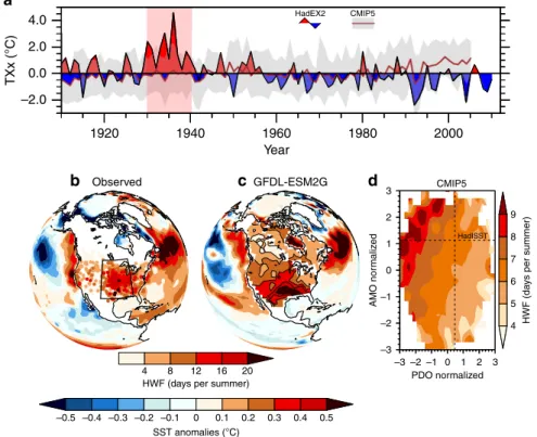
4.0 HadEX2 CMIP5

a

2.0 0.0 –2.0 1920 Observed 4 8 12

HWF (days per summer)

–0.5 –0.4 –0.3 –0.2 –0.1 SST anomalies (°C) 0 0.1 0.2 0.3 0.4 0.5 16 20 3 9 HadISST 8 7 6 5 4 HWF (da ys per summer) CMIP5 2 1 0 –1 –2 –3 –3 –2 –1 PDO normalized 0 1 2 3 AMO nor maliz ed GFDL-ESM2G

b

c

d

1940 1960 Year 1980 2000 TXx (°C)

Fig. 1 Observed and simulated central US summer heatwave activity and associated sea surface temperatures. a Observed summer (June_–August) maximum daily maximum temperature (TXx) anomalies (relative to 1901–2010) averaged over the central US (box in b), from gridded observations (HadEX2; colour), and 20 Coupled Model Intercomparison Project Phase 5 (CMIP5) historical model simulations (grey line with shading indicating the 10–90th percentile range; relative to 1901–2005). b, c Summer sea surface temperature anomaly and heatwave frequency (HWF) patterns averaged across the most active heatwave summer decade (11 years) per century over the central US for station observations (b; pink shade in a), and a selected CMIP5 model (Geophysical Fluid Dynamics Laboratory Earth System Model with Generalised Ocean Layer Dynamics component, GFDL-ESM2G) decade with heatwave activity commensurate with observations (c). d Composite anomalies of central US summer HWF as a function of the normalised annual Pacific Decadal Oscillation (PDO) and Atlantic Multidecadal Oscillation (AMO) indices, from 22 CMIP5 pre-industrial (pi) Control experiments totalling 10,900 years (1930s decadal observations shown as the intersect of dotted lines). The PDO and AMO definition are described in the ‘Methods'.

simulations, we use one pre-industrial (pi) Control experiment

each from 22 CMIP5 models (~500 years per model, see

‘Methods' and Supplementary Table 2). When averaged over

almost 11,000 model years, a multi-model ensemble (MME)

mean of summer heatwave frequency (HWF; total number of

heatwave days) shows that simulated central US heatwaves are

more frequent during a warm AMO phase and a cool PDO phase

(Fig.

1

d). While the simulated PDO phases for higher HWFs do

not match with 1930s observed state, heat extremes

20

_and

drought periods

18

over central and eastern US in the late 1990s to

early 2000s were associated with a similar decadal pattern to the

CMIP5 piControl MME. From the nearly 11,000 CMIP5

piControl years, we identify one decade per century per model

where record-breaking heatwave activity is commensurate with

the 1930s observations. In terms of geographic extent,

record-breaking heatwave activity is rare in the piControl simulations, as

is the clustering of events in a decade (see

‘Methods’). Only one

CMIP5 piControl decade, in GFDL-ESM2G (model years

286–296), breaks HWF records over more than 50% of northern

and southern–central US, similar to observations (Fig.

1

c;

Supplementary Table 2). This simulated decade also features a

warm north Atlantic and anomalously cooler eastern Pacific (i.e.,

warm PDO and AMO phases), indicating that rare Dust

Bowl-like heatwaves can be simulated in the absence of external

forcings like land-cover change and dust. This model is also one

of a minority of CMIP5 models that is able to represent

AMO-like behaviour in its piControl simulation

21

_.

AGCM studies have emphasised the importance of Pacific SST

anomalies to central US droughts

22,23

, even for the 1930s

4,12

.

We separate the influence of Atlantic and Pacific SST anomalies

on the summer heatwaves across the 1930s using AGCM

experiments conducted in HadGEM3-GA6

24

_{for the early}

twentieth century warming period (1916–1955; see ‘Methods'

for the experiment design). This period yields ~15 years of the

data on either side of the 1930s in order to create an extended

climatology to compare the Dust Bowl years against. We define

the Dust Bowl period as 1930–1937 to encompass the summers

with the most extreme heatwave conditions observed in the

1930s

3

_{, and the HadGEM3 ensembles that capture atmospheric}

variability are expected to sample it. We

first look at a HadGEM3

ensemble forced with historical SSTs (HIST). The HIST

ensemble underestimates heatwave activity (comparing Fig.

2

a,

d), and generates well-documented biases in temperature

4,7

_and

heatwave magnitude (average temperature of heatwaves) over the

southern–central US (105°–85°W, 30°–40°N; Supplementary

Fig. 2). Such mean-state temperature biases and anomalous

responses to 1930s SSTs exist in other AGCMs, particularly

over central and southern North America (contours,

Supplemen-tary Fig. 3). Warm model biases over central and southern

North America

25

are thought to be due to overly strong

land–atmosphere coupling which can amplify heat even in wet

regions

26

_{and lead to persistent drought over the Great Plains}

23

_.

Focusing on HWF, a metric defined relative to a model’s own

climatology is a partial solution to this issue; however, biases in

HadGEM3’s physics could still infiltrate and artificially accelerate

heatwave development. This is why improvements in the

parameterisation of land-surface models is critical, particularly

for reducing uncertainty in future climate model projections

27

_.

To separate the influence of the Atlantic (ATL

HIST

) and Pacific

(PAC

HIST

) SSTs, we carry out simulations in which SSTs outside

their respective domain cycle through climatological values.

The resulting patterns from the ATL

HIST

ensemble show a

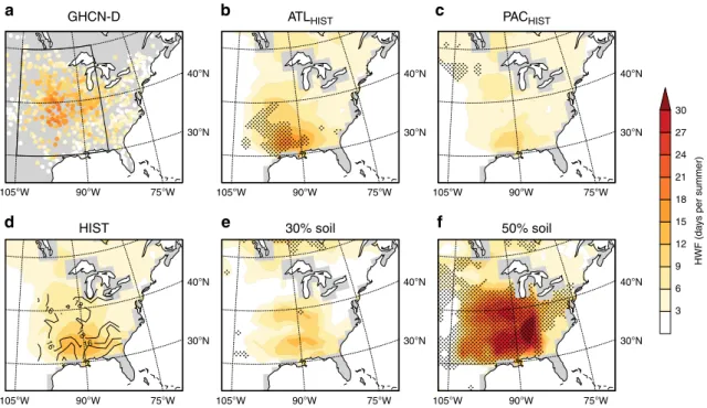
40°N

GHCN-D ATL_HIST

HIST 30% soil 50% soil

PAC_HIST 30°N 105°W 90°W

a

b

c

d

e

f

75°W 40°N 30°N 105°W 90°W 75°W 40°N 30°N 105°W 90°W 75°W 40°N 30°N 105°W 90°W 75°W 40°N 30 27 24 21 18 15 12 9 6 3 HWF (da ys per summer) 30°N 105°W 90°W 75°W 40°N 30°N 105°W 90°W 75°W

Fig. 2 Observed and simulated summer heatwave frequency during the Dust Bowl. Average heatwave frequency (HWF) over the central US for 1930–1937, for observations from Global Historical Climatology Network-Daily (GHCN-D; a), and Hadley Centre Global Environment Model version 3 (HadGEM3) simulations, including afive-member Atlantic sea surface temperature (SST) ensemble (ATLHIST;b),five-member Pacific SST ensemble

(PACHIST;c), ten-member historical SST ensemble (HIST; d), and single-model experiments where the amount of bare soil in 1930, averaged over the

central US, was increased from 15 to 30% (e) and 50% (f). Stippling indicates significantly larger HWF values between (b, c) ATLHISTand PACHIST

ensembles (N = 40) at the 95% confidence level (see ‘Methods')28_{, and in (e, f) HWF values outside the HIST simulation range. Contours in (d) indicate}

the percentage of bare soil in each grid cell over the most active heatwave region in the HIST, ATLHISTand PACHISTmembers. The climatology period is

significantly stronger response in heatwave activity and intensity

across the southern–central US than the PAC

HIST

ensemble (95%

level based on a Mann–Whitney U test

28

_{, Fig.}

₂

_{b, c;}

Supplemen-tary Figs. 1c and

2), consistent with the CMIP5 piControl

analysis highlighting the importance of Atlantic SSTs (Fig.

1

).

How continental US surface temperatures respond to remote

SSTs varies across AGCMs

22

_{and coupled models}

23

_{, and often}

depends on a models’ middle to upper-level circulation response

to SST forcing, particularly over the southern US

5,29

.

Role of summer circulation. The spatial extent and amplitude of

the hottest heatwaves varied considerably during the 1930s

3

_{, yet}

events often coincided with a persistent high mean sea-level

pressure (MSLP) anomaly over the western US (Fig.

3

a), coupled

with a mid-tropospheric ridge

5,6

_{. One possibility is that the}

summer atmospheric circulation response to SST anomalies was

the main contributor to the heatwave activity. To test if this

explains the stronger ATL

HIST

heatwave response, we examine

the daily atmospheric circulation at the surface (i.e., MSLP) and

in the mid-troposphere (i.e., 500 hPa geopotential heights; Z500)

during the hottest heatwave weeks for each summer across the

simulations (see

‘Methods'). For the HIST ensemble, it captures

the observed mid-tropospheric ridge across the eastern US

associated with the hot conditions over the central US, which is

coupled to a surface low anomaly at 100°W, 45°N (Fig.

3

b). The

heat low and upper-level ridge anomalies are also prominent

features in the ATL

HIST

ensemble (Fig.

3

c); however, the surface

high anomaly in the western US is absent. In the PAC

HIST

ensemble, the upper-level ridge is placed further northwards

(50°–60°N), while the surface low anomaly is considerably weaker

and displaced southwards over the southeast US coast (Fig.

3

d),

consistent with a more muted heatwave response. This suggests

that for HadGEM3, the main circulation features associated

with the hottest Dust Bowl heatwaves across the eastern US

are best reproduced with an Atlantic SST forcing. Yet the

summer heatwave circulation differences (Δ[ATL

HIST

, PAC

HIST

])

over the central US are not significantly different (based on

Kolmogorov–Smirnov two-sample test; also see Supplementary

Fig. 4e, f) and cannot fully explain the summer heatwave intensity

differences between the ATL

HIST

and PAC

HIST

ensembles. We

turn to the role of dry springs in the lead up to the Dust Bowl

summers.

Dry spring preconditioning summer heatwaves. A key factor in

observed summer heat extremes over the Great Plains is

spring-time preconditioning

6

_{. Observational studies suggest that}

dry springs pre-conditioned the Dust Bowl summer heat

extremes

3,6,10

_{, driven, in part, by mid-tropospheric ridging}

10

_and

reduced moisture advection from the Gulf of Mexico

9

_{. Prior to}

summer, significant April–May precipitation deficits emerge

throughout the southern–central US in the ATL

HIST

ensemble

compared to PAC

HIST

(Fig.

4

a). The largest precipitation deficit

for ATL

HIST

occurs mid-May (Supplementary Fig. 4a) and

cor-responds to comparatively lower evaporative fractions, higher

daily Tmax (although no difference in Tmin

30

_{) and a deeper}

surface low throughout the summer months (Supplementary

Fig. 4b, c, e). The drier and hotter ATL

HIST

ensemble conditions

also partially reflect the weaker meridional moisture fluxes from

the Gulf of Mexico in April–May (Fig.

4

a; Supplementary

Fig. 4d), reminiscent of the observed 850 hPa wind anomalies in

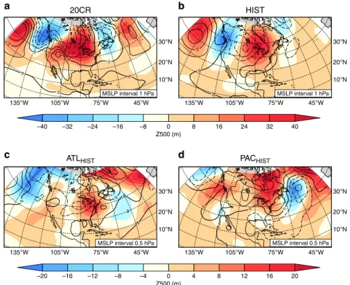
20CR 135°W –40 –32 –24 –16 –8 0 Z500 (m) 8 16 24 32 40 –20 –16 –12 –8 –4 0 Z500 (m) 4 8 12 16 20 105°W 75°W

MSLP interval 1 hPa MSLP interval 1 hPa

MSLP interval 0.5 hPa MSLP interval 0.5 hPa

45°W 135°W 105°W 75°W 45°W 135°W 105°W 75°W 45°W 135°W 105°W 75°W 45°W 30°N 20°N 10°N 30°N 20°N 10°N 30°N 20°N 10°N 30°N 20°N 10°N

ATLHIST PACHIST

HIST

a

b

c

d

Fig. 3 Atmospheric conditions during the hottest Dust Bowl heatwaves. The spatial patterns of mean sea-level pressure (MSLP; colours) and geopotential height at 500 hPa (Z500; contours), averaged over a 7-day period from the start of the hottest summer heatwave over the central US, and averaged over 1930–1937. Shown are the twentieth century reanalysis version 2c (20CR; a), a ten-member Hadley Centre Global Environment Model version 3 (HadGEM3) historical sea surface temperature (SST) ensemble mean (HIST;b), a_{five-member Atlantic SST ensemble mean (ATL}HIST;c), and a

five-member Pacific SST ensemble mean (PACHIST;d). The thick line indicates the 0 hPa MSLP anomaly, while the solid (dashed) lines indicate positive

(negative) MSLP anomalies.

spring during the mid-1930s

6

_{. While it appears difficult to}

dis-tinguish the absolute mid-tropospheric circulation (e.g., Z500)

over the eastern US between the idealised SST HadGEM3

ensembles (Supplementary Fig. 4f), the ATL

HIST

ensemble Z500 is

consistently higher than the PAC

HIST

ensemble by 5–15 m over

March–May. Hence, warm Atlantic SST anomalies are more

conducive to forcing stronger mid-tropospheric ridging in spring

during the 1930s. This weakens the northward moisture

fluxes,

driving a precipitation deficit and a drying which extends to

summer, forcing more active and intense heatwave conditions

3,6

_.

It is well established that systematic regional precipitation

biases exist in AGCMs simulating the Dust Bowl drought

4,7,8,12

.

This is true of HadGEM3 and three other AGCMs that have

conducted 1930s historical SST-forced experiments and simulate

wet spring biases (Supplementary Fig. 5). Even with HadGEM3’s

wet bias, ATL

HIST

exhibits comparatively stronger precipitation

deficits in mid-spring to summer (than PAC

HIST

), and lower

evaporative fractions, consistent with an overly responsive

land–atmosphere coupling, in line with other models

26,31

_{. The}

majority of forecast systems also overestimate the relationship

between dry late springs and summer heat biases due to an

excessive reduction in soil moisture

30

_{. The warm bias in}

HadGEM3 further causes overly deep surface low anomalies

from July (Supplementary Fig. 4e), which exacerbate the average

Dust Bowl heatwave temperatures (Supplementary Fig. 2).

In overestimating the land–atmosphere coupling strength,

HadGEM3 dries out too rapidly in late spring, yet processes

controlling the heatwave development can still be compared

between differently forced simulations

10,22,29

_{. Other important}

processes, such as land-cover changes

4,13

_{in the 1930s, are}

examined next.

Role of land-cover changes. Although the role of SSTs in

trig-gering the Dust Bowl Drought is recognised

11

, land-cover

chan-ges likely amplified the heatwaves

13

_{. Land-cover changes across}

the US Great Plains in the 1920s and 1930s included widespread

crop failures surpassing 60% in many counties

32

. Estimates of the

amount of bare soil range from 20 to 80%, depending on regions

with or without erosion

13

_{, with AGCMs likely underestimating}

the true amount

4

. In order to evaluate the contribution by

land-cover changes, we conducted sensitivity experiments using

Had-GEM3, in which temperate C3 and tropical C4 grass cover over

the central US-wide was converted to bare soil. This represents

the repeated crop failure

4,32

during the 1930s that led to soil

exposure and expansive and rapid loss of top soil

10

_{. In three}

separate model experiments, the percentage of bare soil averaged

over the central US in 1930 was increased from an approximate

15% reference fractional extent to 30%, 50 and 80%, at the

expense of C3 and C4 grass. This represents a percentage loss of

grass, averaged over the central US in 1930, of 25%, 50% and

100% (Supplementary Fig. 6), which is restored to HIST fractions

by 1940 (see

‘Methods' and Supplementary Fig. 7). As a

com-parison, Cook et al.

4

used a conservative estimate of up to 50%

devegetation in some grid boxes in their 1930s simulations. Our

experiments reveal a significant increase in HWF from around

6 days in the 30% soil experiment (Fig.

2

e) to ~17 days in the 50%

run (Fig.

2

f), eventually reaching an average of 33 days per

summer in the 80% run over the southern–central US

(Supple-mentary Fig. 2). With more exposed bare soil, an earlier

eva-poration deficit appears to drive the elevated heatwave response

through soil desiccation, despite only minor differences in

pre-cipitation between the 50% and 80% soil experiments (Fig.

4

c, d).

Reductions in early summer soil moisture and latent heat

fluxes

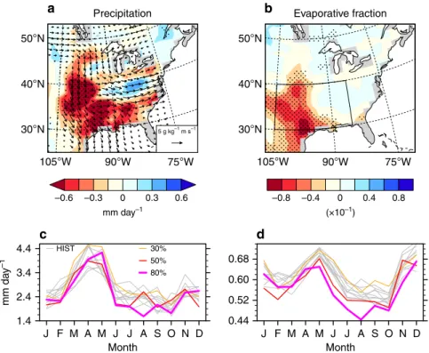
Precipitation Evaporative fraction

50°N

a

c

d

b

40°N 30°N 105°W 4.4 0.68 0.60 0.52 0.44 HIST 30% 50% 80% 3.4 2.4 1.4 mm da y –1 J F M A M J Month J A S O N D J F M A M J Month J A S O N D –0.6 –0.3 0 0.3 0.6 –0.8 –0.4 0 0.4 0.8 mm day–1 (×10–1) 90°W 75°W 50°N 40°N 30°N 105°W 90°W 75°W 5 g kg–1 m s–1

Fig. 4 Late spring conditions prior to the Dust Bowl summers. a, b, Composite differences in April–May conditions between the five-member Atlantic sea surface temperature (SST) ensemble mean (ATLHIST) andfive-member Pacific SST ensemble mean (PACHIST) prior to the Dust Bowl summers for

1930–37. The fields shown are precipitation (colours; a) and 850 hPa moisture flux (vectors; a) and evaporative fraction (b). Stippling on precipitation and evaporative fraction contours indicates significance above the 95% confidence level based on a bootstrap mean difference on 10,000 × 8 April–May samples (resampled).c, d Annual cycle of precipitation (c) and evaporative fraction (d) for the ten-member historical SST members (HIST) and bare-soil model experiments averaged over 1930–1937 and the southern–central US (region in (b); 105°–85°W, 30°–40°N).

provide further evidence of an earlier drought emergence under

increasing crop removal, leading to a thicker atmospheric

boundary layer (Supplementary Fig. 8e–g). A more dramatic

HWF response in the heavily forested areas to the south

33

_than

the grasslands to the north and west, stems from the smaller

diurnal temperature variations in the tropical latitudes. This has a

larger effect on HWF as the heatwave threshold is easier to

exceed, and hence a small increase in summer temperatures can

lead to a larger HWF signal than over a region with more variable

summer temperatures

14

_{. Part of bare-soil induced heatwave}

impacts stem from greater temperature advection along the Gulf

regions, although this occurs mainly along the coast.

High-resolution modelling experiments suggests the primary role that

land-cover changes had in amplifying the Dust Bowl drought was

by reducing the moisture transport to the central US

13

; however,

we

find little appreciative change in moisture fluxes

(Supple-mentary Fig. 8b). Other studies have shown elevated 1930s dust

aerosols

4,11

would have suppressed precipitation through

land–atmosphere feedbacks although these studies excluded the

indirect aerosol effect on cloud microphysics. We see no evidence

of land albedo differences in our bare-soil experiments

(Supple-mentary Fig. 8h), despite the high dust loadings (Supple(Supple-mentary

Fig. 6), although it is possible that precipitation efficiency is

reduced via the dust-radiative effects on clouds

34

. Our results

suggest that regional-scale land-surface processes play a more

dominant role over the large-scale atmospheric dynamics and

land–atmosphere feedbacks in our bare-soil experiments. If

HadGEM3 had a more accurate spatial and temporal

repre-sentation of the 1930s land cover

13

_{that distinguished the less}

drought-resilient dryland crops (due to their shallower root

sys-tem), this may have produced more realistic heatwaves, yet it

would still not capture important land–atmosphere feedbacks

that result from increased soil erosion and elevated dust levels

4,11

_.

Discussion

Supported by the HadGEM3 results (Fig.

2

) and consistent with

unforced CMIP5 simulations (Fig.

1

), this study reveals that

Atlantic SSTs were an important factor in the Dust Bowl

heat-waves, enhancing spring drought, and allowing heat to develop

earlier over the central US

3,6

_{. Pacific SSTs played less of a role in}

the heatwave development, at least in our AGCM simulations

(Fig.

2

), but have been shown to contribute to the Dust Bowl

drought in other AGCMs

7,8

and more generally, to long-term

droughts over the Great Plains in coupled models

23

_{. Yet AGCMs}

forced with observed SSTs alone or historical boundary

condi-tions remain far from quantitatively reproducing the exceptional

nature of the Dust Bowl heatwaves (or drought) (e.g., Fig.

2

). This

is likely stems from how models treat 1930s land-cover changes,

resulting from rapid deep plowing of native grassland.

Sub-sequent drought brought about widespread crop failures

32,35

_{, dust}

storms

36

_{and protracted heatwaves}

3

_{. Despite the uncertainty}

behind the exact amount of devegetation prior to and during the

1930s

4,32

_{(see Soil Conservation Service erosion map}

37

_{), our grass}

devegetation experiments show a strong enhancement in

heat-wave activity and intensity (i.e., absolute maximum temperatures)

as bare-soil amounts increase. This is due to a greater partitioning

of surface energy

fluxes to sensible heat and a rapid drying of

exposed soil (Fig.

4

), although elevated dust loads appear not to

suppress precipitation in HadGEM3 as in other AGCMs

11

. The

1930s extreme heatwaves serve as a reminder that vegetation

feedbacks from a greenhouse gas-induced warming, resulting

from human activities, could lead to the enhancement of extreme

heatwaves and drought triggered by decadal climate variability.

Even with recent crop intensification linked to cooler and wetter

conditions over the central US

38

, major crop losses would likely

still occur if future Dust Bowl-like heatwaves eventuate

35,39

_due

to a warmer world.

Methods

Heatwave metrics and surface heatfluxes. The use of consecutive hot days and nights (3 days for Tmax and 2 nights for Tmin) above their respective daily 90th percentile threshold is similar to other heatwave definitions15_{. The threshold is}

calculated over the full climatological period, using a centred 15-day window that removes monthly and seasonal dependencies. Heatwave metrics are then separated into two categories: (1) activity; total number of summer heatwave days (frequency; HWF), and longest summer heatwave event (duration; HWD); and (2) intensity; average temperature of all summer heatwaves (magnitude; HWM). As we do not study the human health impact, we do not consider relative humidity (increasing the heat stress40_{) in our heatwave definition. Even with the lack of reliable humidity}

observations in the 1930s41_{, the study’s main focus is on the record heat, and its}

association with SSTs and bare soil. We acknowledge HadGEM3 contains a strong warm bias in summer hot extremes and a wet spring bias over North America, along with other AGCMs (see Supplementary Figs. 2, 5), most likely due to an over-active land–atmosphere coupling26_{. As such, we primarily focus on HWF as}

this metric partially accounts for warm model biases, as temperatures are refer-enced to a model’s own climatology.

Evaporative fraction (EF) is used as a proxy for soil moisture, calculated from latent (Qe) and sensible (Qh) heatfluxes as EF = Qe/(Qe+ Qh). EF is the ratio of

incoming energy used for evapotranspiration to the total amount of incoming energy. A more arid surface typically has lower EF values and this reduces evaporative cooling42_{; however, the interactions between soil moisture and EF can}

be modulated by daily net radiation and meteorological conditions43_.

Observational and reanalysis data. Daily temperature observations are from the Global Historical Climatology Network-Daily (GHCN-D) archive44_{. Further details}

on the extensive coverage in the 1930s and the station selection can be found in Cowan et al.3_{. Maximum daily Tmax anomalies in Fig.1a are taken from the}

gridded HadEX2 dataset6_{(for a HWF-based version of Fig.1a, see Supplementary}

Fig. 1a). Our hottest heatwave dates were determined from temperatures obtained from the Berkeley Earth Surface Temperature (BEST) dataset45_{, which incorporate}

the large network of GHCN-D stations (Supplementary Fig. 2a shows a HWM comparison between BEST and GHCN-D). Given the daily BEST product is considered experimental, we predominantly focus on GHCN-D for the spatial representation of the observed heatwaves. Daily mean sea-level pressure (MSLP) and 500 hPa geopotential height (Z500)fields are from the US National Oceanic and Atmospheric Administration’s (NOAA) Twentieth Century Reanalysis (20CR) version 2c46_{; the reanalysis product assimilates daily observations of surface}

pressure with monthly SSTs and sea ice as boundary conditions from Hadley Centre Sea-Ice and Sea-Surface Temperature Data Set Version 1 (HadISST1). Monthly precipitation is taken from both GHCN-D and Global Precipitation Climatology Centre (GPCC)47_{, as precipitation (and surface heatfluxes) from}

20CR contain an abundance of artificial inhomogeneities over the central US prior to the 1950s arising from changes in observational density48_.

HadGEM3-GA6 SST-forced experiments. The SST-forced atmospheric model experiments are generated using the HadGEM3-GA6 model with a N96 (~210 km at equator, 135 km at 40°N) horizontal resolution (1.25° × 1.875° and 38 vertical levels in the atmosphere). It is based on the Met Office Unified Model Global Atmosphere 6.0 (Version 8.5) and Joint UK Land Environment Simulator (JULES) land-surface model 6.024_{. HadGEM3 is driven by observed daily SSTs, interpolated}

from monthly values from HadISST2.1, which contains a more comprehensive coverage of in situ observations and more complete bias corrections than HadISST117_.

The HadGEM3 experimental set-up comprises of ten historical simulations (HIST) run over 1916–1955 with each member forced with a different SST realisation that encompasses observational uncertainties and bias adjustments49

and standard CMIP5 historical drivers (e.g., well-mixed greenhouse gases, aerosols, land-use changes). A further two sets offive idealised simulations were conducted: thefirst set kept Atlantic SST anomalies at historical observed values (ATLHIST),

while the second set kept Pacific SST anomalies at historical observed values (PACHIST). In both ensembles, the remaining oceans cycled through a 1916–1955

climatology for each year, with anomalies joining at 50°S and 60°N, far from the region of interest. The SST and ice regions below and above the aforementioned latitudes are kept at climatology in both experiment ensembles. The residual response was computed as the difference between the ATLHISTand PACHIST

ensembles following the approach of Schubert et al.7_{. All model-based heatwave}

metrics are calculated relative to the ten-member HIST ensemble climatology from 1916–1955. HadGEM3’s HIST mean-state precipitation and surface temperature are within the range of three other AGCMs that have conduced similar SST-forced experiments (Supplementary Figs. 3, 5). The three comparison AGCMs are GFDL-AM3 (~1.9° × 1.9° horizontal resolution), GEOS-5 (1.25° × 1° resolution) and ESRL-CAM5 (0.5° × 0.5° resolution). The warm bias in over the southern–central US in HadGEM3 is accentuated in the soil experiments with maximum

temperatures ranging from 43 °C to 52 °C (Supplementary Fig. 8a), compared with observed temperatures of 32–34 °C.

HadGEM3-GA6 bare-soil experiments. Each land grid cell consists of different fractions of surface types, like grass, bare soil, trees and shrubs. Devegetation experiments were generated by converting C3 (temperate) and C4 (tropical) grassland fractions over the central US to bare soil. The land fraction ancillaryfiles are linearly interpolated between decades, meaning values are given every decade (e.g., 1920, 1930, 1940). The soil experiments are labelled 30%, 50% and 80% soil, which refers to the approximate percentage of bare soil in 1930 averaged over the central US (base soil percentage in HIST is 15.3%). The equivalent combined C3 and C4 grass loss, averaged over the central US at 1930 for the three experiments, is ~25%, 50% and 100% (Supplementary Fig. 6). This subsequently increases the dust aerosol load in the spring season over the same region. In each of these experi-ments, the bare-soil percentage returns to 15.3% by 1940, meaning the temporal rate of grass recovery differs between the three experiments during the 1930s decade (Supplementary Fig. 7). For comparison, Cook et al.4_{use up to a 50%}

vegetation loss over particular grid points in similar experiments in the GISS ModelE over the central US Great Plains (105°–95°W, 30°–50°N), which they assume to be a conservative estimate due to the exclusion of natural vegetation loss during the Dust Bowl drought. Only one soil sensitivity experiment is conducted per soil fraction, and as such, given the lack of multiple ensemble members, sta-tistical significance is based on whether a grid point lies outside the ten-member HIST range. For example, the HIST mean summer mean surface temperature for the southern Great Plains over 1930–1937 ranges from 30.2 °C to 31.3 °C across the ensemble members, whereas the 50% and 80% soil experiment temperatures of 32.8 °C and 35.5 °C, respectively, exceed the HIST range, and therefore are deemed to be statistically significant. As the bare-soil sensitivity experiments are rudi-mentary in their design, the aim was not to realistically quantify their imprint on the Dust Bowl heatwaves, but to gauge the impact devegetation can have on the amplification of heatwaves and to test for land-atmospheric feedbacks. As with previous studies using land-cover estimates from the 1930s4,13_{, the assumptions of}

bare soil amounts remain subjective.

Circulation patterns. For the reanalysis and each model simulation, wefind the dates of the hottest summer heatwave week over the central US. To achieve this, for each grid cell and each summer, wefirst calculated the heatwave start date using the heatwave amplitude (i.e., the hottest day of the hottest heatwave), and then determined how many grid cells shared the same date. A 7-day running mean was performed over all start dates to choose the week with the largest percentage of central US grid cells that shared the same heatwave start date (centred in the week). We then average each simulation’s MSLP and Z500 over the hottest heatwave week and over 1930–1937 to create the composites shown in Fig.3. Each composite is made up of 7 days × 8 years × 5 (or 10) experiments, leading to 280 patterns for ATLHIST, PACHISTand 560 patterns for HIST.

CMIP5 experiments. Heatwave metrics, calculated from daily Tmax and Tmin, and monthly SSTs were analysed from the piControl experiments of 22 CMIP5 models50_{(Supplementary Tables 1, 2). All model data were interpolated onto a}

regular 1° grid prior to analysis. Models with at least 400 piControl years of output were considered (all except for bcc-csm1-1-m have 500 years), which allowed for an assessment of multiple occurrences of record-breaking heatwaves over at least four centuries for each individual model piControl experiment. To ensure we captured decadally clustered events as observed during the Dust Bowl decade, rather than outlier record-breaking heatwaves, for each models’ HWF, we applied an 11-year (summer) running average over each central US grid point for the entire piControl period. For each century (e.g., years 1–100, years 101–200, to years 401–500), we selected the maximum HWF value for each grid point and noted the decade of occurrence. We then determined the percentage of central US grid points where record-breaking values fell into the same decade, with the highest percentage selected as the record-breaking decade for that century for that parti-cular model. If two record-breaking heatwave decades occurred within a 30-year time span (e.g., end of one century and beginning of the next), the second decade was ignored to reduce possible contamination from the same decadal SST pattern. This process produced 103 individual piControl heatwave decades. The years when record-breaking heatwaves occurred based on HWF and centred on the decade in question, and the percentage area of the central US impacted, are shown for each CMIP5 model in Supplementary Table 2. The GFDL-ESM2G model is highlighted in Fig.1as an example of one such model decade that realistically matches the observations in terms of its SST patterns and heatwave activity (e.g., it breaks similar HWF records over a large spatial extent of the central US, as seen in the 1930s). To test if the simulated heatwave peaks are actually decadal in nature and not random occurrences, we conducted bootstrapping analysis on the CMIP5 piControl runs (10,000 times with replacement) for clusters of at least four sig-nificant heatwave years in a decade that surpass one-standard deviation above the long-term mean. For a heatwave metric like duration, of the 21 CMIP5 models with 500 piControl years, 11 models exhibit decadal cluster frequencies above the bootstrapped third quartile, with six at or above the 95th percentile. This infers that

substantial decadal clustering similar to the 1930s, occurs in about half the models, and strongly in less than 30% of models. These results are similar using heatwave amplitude.

For the historical experiments, we selected 20 CMIP5 models (first run only) to assess the heatwave behaviour and maximum daily Tmax in the historical period simulations (Fig.1a; Supplementary Fig. 1a). These include the 17 CMIP5 models listed in Supplementary Table 2, as well as CCSM4, IPSL-CM5A-MR and GFDL-CM3 (these three models did not have piControl experiments available). The multi-model ensemble mean shows the forced response on HWF (representing heatwave activity) and HWM anomalies (representing heatwave intensity). We would expect to see an increase in the 1930s as there was a large enough forced response in temperature extremes to land-cover changes (i.e., signal to noise), however CMIP5 models are unable to capture these extremes as represented by maximum daily Tmax anomalies (Fig.1a). An increase in irrigation, not included in CMIP5 models51_{, through intense agriculture over the eastern Great Plains is}

thought to be related to a lack of a trend in summer temperatures52_{, compared to}

CMIP5 models since the 1950s (Supplementary Fig. 1a).

The Pacific Decadal Oscillation (PDO) and Atlantic Multidecadal Oscillation (AMO) annually averaged time series were calculated for the same piControl period as the heatwave metrics using NCAR’s Climate Variability Diagnostics Package Repository. The PDO is defined as the leading Principle Component of North Pacific (20–70°N, 110°E–100°W) area-weighted SST anomalies (with global mean SST anomalies removed). The AMO is defined as area-weighted SST anomalies averaged over the North Atlantic (0–60°N, 80°W–0°E), with the global (60°S–60°N) mean SST anomaly removed. No low-pass filtering is performed on the decadal oscillation indices. We included all available CMIP5 models in our multidecadal analysis, although we are aware that the majority of models lack internally generated Atlantic multidecadal variability53_.

Significance tests. In Fig.2, the non-parametric two-tailed Mann–Whitney U

test28_{is used to test the significance in heatwave differences between the ATLHIST}

and PACHISTensembles for each grid point. The null hypothesis tested here is that

the data from ATLHISTand PACHISThave been drawn from the same distribution.

The Mann–Whitney U test determines whether the experiment in question is distinguishable from its partner experiment at the 95% confidence level. The Mann–Whitney U test is conducted on the 1930–1937 heatwave summers metrics, per ensemble member, totalling 80 separate cases (8 events per member ×5 experiment members ×2 experiments). Significance for the precipitation and eva-porative fraction (Fig.4) is tested using a bootstrapping method54_{, whereby}

Had-GEM3 experiment members for either ATLHISTor PACHISTare concatenated to

form 200 samples of the same month, made up of 5 members ×40 years (1916–1955). Differences between two months from the 200 month sample are randomly resampled 10,000 times and significance are detected if the Δ(ATLHIST,

PACHIST) residual lies outside 2.5–97.5% confidence bounds of the resampled

distribution. The significance is unaffected if choosing anomalies or the mean states for the difference calculation.

Data availability

The 20CR circulation variables of Z500 and MSLP can be downloaded athttps://www.esrl. noaa.gov/psd/data/gridded/data.20thC_ReanV2c.html. Daily temperature and precipitation data are from the GHCN-Daily archive are available fromhttp://www1.ncdc. noaa.gov/pub/data/ghcn/daily. Daily SSTs from HadISST2.1 are available on request. Monthly precipitation from GPCC are available fromhttps://www.esrl.noaa.gov/psd/data/ gridded/data.gpcc.html. The HadGEM3 experiments are available on request. The CMIP5 piControl experiments are available viahttps://esgf-node.llnl.gov/projects/cmip5, and can be downloaded with a valid Earth Systems Grid account. The AMO and PDO time series from the CMIP5 piControl simulations can be downloaded from NCAR’s Climate Variability Diagnostics Package Repository:http://www.cesm.ucar.edu/working_groups/ CVC/cvdp/data-repository.html. The comparison AGCMs can be obtained fromhttps:// psl.noaa.gov/courtesy of the NOAA-ESRL Physical Sciences Laboratory.

Code availability

The code to generate thefigures is available athttps://github.com/tcowan80/ Cowan_et_al_2020_DustBowl_HadGEM3, and is based on the NCAR Command Language (version 6.6.2; doi:10.5065/D6WD3XH5). The code to generate climatologies was constructed using Climate Data Operators (CDO) version 1.9.8.

Received: 3 November 2019; Accepted: 15 May 2020;

References

1. NOAA National Centers for Environmental Information, State of the Climate: National Climate Report for August 2019,https://www.ncdc.noaa.gov/sotc/ national/201908(2019).

2. Abatzoglou, J. T. & Barbero, R. Observed and projected changes in absolute temperature records across the contiguous United States. Geophys. Res. Lett. 41, 6501–6508 (2014).

3. Cowan, T. et al. Factors contributing to record-breaking heat waves over the Great Plains during the 1930s Dust Bowl. J. Clim. 30, 2437–2461 (2017). 4. Cook, B. I., Miller, R. L. & Seager, R. Amplification of the North American

‘Dust Bowl’ drought through human-induced land degradation. Proc. Natl Acad. Sci. USA 106, 4997–5001 (2009).

5. Cook, B. I., Seager, R. & Miller, R. L. Atmospheric circulation anomalies during two persistent north american droughts: 1932–1939 and 1948–1957. Clim. Dyn. 36, 2339–2355 (2011).

6. Donat, M. G. et al. Extraordinary heat during the 1930s US Dust Bowl and associated large-scale conditions. Clim. Dyn. 46, 413–426 (2016).

7. Schubert, S. D., Suarez, M. J., Pegion, P. J., Koster, R. D. & Bacmeister, J. T. On the cause of the 1930s Dust Bowl. Science 303, 1855–1859 (2004). 8. Seager, R. et al. Would advance knowledge of 1930s SSTs have allowed

prediction of the Dust Bowl drought? J. Clim. 21, 3261–3281 (2008). 9. Brönnimann, S. et al. Exceptional atmospheric circulation during the‘Dust

Bowl’. Geophys. Res. Lett. 36, L08802 (2009).

10. Cook, B. I., Seager, R. & Smerdon, J. E. The worst North American drought year of the last millennium: 1934. Geophys. Res. Lett. 41, 7298–7305 (2014). 11. Cook, B. I., Miller, R. L. & Seager, R. Dust and sea surface temperature forcing of the 1930s“Dust Bowl” drought. Geophys. Res. Lett. 35, L08710 (2008). 12. Hoerling, M., Quan, X. & Eischeid, J. Distinct causes for two principal U. S.

droughts of the 20th century. Geophys. Res. Lett. 36, L19708 (2009). 13. Hu, Q., Torres-Alavez, J. A. & Van Den Broeke, M. S. Land-cover change and

the‘Dust Bowl’ drought in the U.S. Great Plains. J. Clim. 31, 4657–4667 (2018). 14. Perkins-Kirkpatrick, S. E. & Gibson, P. B. Changes in regional heatwave

characteristics as a function of increasing global temperature. Sci. Rep. 7, 12256 (2017).

15. Grotjahn, R. et al. North American extreme temperature events and related large scale meteorological patterns: a review of statistical methods, dynamics, modeling, and trends. Clim. Dyn. 46, 1151–1184 (2016).

16. Nigam, S., Guan, B. & Ruiz-Barradas, A. Key role of the Atlantic Multidecadal Oscillation in 20th century drought and wet periods over the Great Plains. Geophys. Res. Lett. 38, L16713 (2011).

17. Tokinaga, H., Xie, S.-P. & Mukougawa, H. Early 20th-century Arctic warming intensified by Pacific and Atlantic multidecadal variability. Proc. Natl Acad. Sci. USA 114, 6227–6232 (2017).

18. McCabe, G. J., Palecki, M. A. & Betancourt, J. L. Pacific and Atlantic Ocean influences on multidecadal drought frequency in the United States. Proc. Natl Acad. Sci. USA 101, 4136–4141 (2004).

19. Hegerl, G. et al. Causes of climate change over the historical record. Environ. Res. Lett. 14, 123006 (2019).

20. McKinnon, K. A., Rhines, A., Tingley, M. P. & Huybers, P. Long-lead predictions of eastern United States hot days from Pacific sea surface temperatures. Nat. Geosci. 9, 389–396 (2016).

21. Mann, M. E., Steinman, B. A. & Miller, S. K. Absence of internal multidecadal and interdecadal oscillations in climate model simulations. Nat. Commun. 11, 49 (2020).

22. Schubert, S. et al. A U.S. Clivar project to assess and compare the responses of global climate models to drought-related SST forcing patterns: overview and results. J. Clim. 22, 5251–5272 (2009).

23. McCrary, R. R. & Randall, D. A. Great Plains drought in simulations of the twentieth century. J. Clim. 23, 2178–2196 (2010).

24. Walters, D. et al. The Met Office Unified Model Global Atmosphere 6.0/6.1 and JULES Global Land 6.0/6.1 configurations. Geosci. Model Dev. 10, 1487–1520 (2017).

25. Mueller, B. & Seneviratne, S. I. Systematic land climate and evapotranspiration biases in CMIP5 simulations. Geophys. Res. Lett. 41, 128–134 (2014). 26. Ukkola, A. M., Pitman, A. J., Donat, M. G., De Kauwe, M. G. & Angélil, O.

Evaluating the contribution of land-atmosphere coupling to heat extremes in CMIP5 models. Geophys. Res. Lett. 45, 9003–9012 (2018).

27. Donat, M. G., Pitman, A. J. & Angélil, O. Understanding and reducing future uncertainty in midlatitude daily heat extremes via land surface feedback constraints. Geophys. Res. Lett. 45, 10,627–10,636 (2018).

28. Mann, H. B. & Whitney, D. R. On a test of whether one of two random variables is stochastically larger than the other. Ann. Math. Stat. 18, 50–60 (1947).

29. Ruprich-Robert, Y. et al. Impacts of the Atlantic multidecadal variability on North American summer climate and heat waves. J. Clim. 31, 3679–3700 (2018). 30. Ardilouze, C. et al. Multi-model assessment of the impact of soil moisture

initialization on mid-latitude summer predictability. Clim. Dyn. 49, 3959–3974 (2017).

31. Sippel, S. et al. Refining multi-model projections of temperature extremes by evaluation against land-Atmosphere coupling diagnostics. Earth Syst. Dyn. 8, 387–403 (2017).

32. Gutmann, M. P. et al. Migration in the 1930s: Beyond the Dust Bowl. Soc. Sci. Hist. 40, 707–740 (2016).

33. Steyaert, L. T. & Knox, R. G. Reconstructed historical land cover and biophysical parameters for studies of land-atmosphere interactions within the eastern United States. J. Geophys. Res. Atmos. 113, D02101 (2008). 34. Lohmann, U. & Feichter, J. Global indirect aerosol effects: a review. Atmos.

Chem. Phys. 5, 715–737 (2005).

35. Glotter, M. & Elliott, J. Simulating US agriculture in a modern Dust Bowl drought. Nat. Plants 3, 16193 (2016).

36. Worster, D. Dust Bowl: The Southern Plains in the 1930s (Oxford University Press, 1979).

37. Soil Conservation Service. US Department of Agriculture Map 2579.https:// www.nrcs.usda.gov/wps/portal/nrcs/detail/national/about/history/? cid=stelprdb1049437(1954).

38. Mueller, N. D. et al. Cooling of US Midwest summer temperature extremes from cropland intensification. Nat. Clim. Chang. 6, 317–322 (2016). 39. Cowan, T., Undorf, S., Hegerl, G. C., Harrington, L. J. & Otto, F. E. L.

Present-day greenhouse gases could cause more frequent and longer Dust Bowl heatwaves. Nat. Clim. Chang.https://doi.org/10.1038/s41558-020-0771-7

(2020).

40. Sherwood, S. C. How Important Is Humidity in Heat Stress? J. Geophys. Res. Atmos. 123, 11,808–11,810 (2018).

41. Brown, P. J. & DeGaetano, A. T. Trends in U.S. surface humidity, 1930–2010. J. Appl. Meteorol. Climatol. 52, 147–163 (2013).

42. Donat, M. G., Pitman, A. J. & Seneviratne, S. I. Regional warming of hot extremes accelerated by surface energyfluxes. Geophys. Res. Lett. 44, 7011–7019 (2018).

43. Ford, T. W., Wulff, C. O. & Quiring, S. M. Assessment of observed and model-derived soil moisture-evaporative fraction relationships over the United States Southern Great Plains. J. Geophys. Res. Atmos. 119, 6279–6291 (2014).

44. Menne, M. J., Durre, I., Vose, R. S., Gleason, B. E. & Houston, T. G. An overview of the Global Historical Climatology Network-Daily database. J. Atmos. Ocean. Technol. 29, 897–910 (2012).

45. Rohde, R. et al. A new estimate of the average Earth surface land temperature spanning 1753 to 2011. Geoinfor. Geostat. Overview 1, 1–7 (2013). 46. Compo, G. P. et al. The Twentieth Century Reanalysis project. Q. J. R.

Meteorol. Soc. 137, 1–28 (2011).

47. Becker, A. et al. A description of the global land-surface precipitation data products of the Global Precipitation Climatology Centre with sample applications including centennial (trend) analysis from 1901-present. Earth Syst. Sci. Data 5, 71–99 (2013).

48. Ferguson, C. R. & Villarini, G. An evaluation of the statistical homogeneity of the Twentieth Century Reanalysis. Clim. Dyn. 42, 2841–2866 (2014). 49. Titchner, H. A. & Rayner, N. A. The Met Office Hadley Centre sea ice and sea

surface temperature data set, version 2: 1. Sea ice concentrations. J. Geophys. Res. Atmos. 119, 2864–2889 (2014).

50. Taylor, K. E., Stouffer, R. J. & Meehl, G. A. An overview of CMIP5 and the experiment design. Bull. Am. Meteorol. Soc. 93, 485–498 (2012).

51. Cook, B. I., Shukla, S. P., Puma, M. J. & Nazarenko, L. S. Irrigation as an historical climate forcing. Clim. Dyn. 44, 1715–1730 (2015).

52. Alter, R. E., Douglas, H. C., Winter, J. M. & Eltahir, E. A. B. Twentieth century regional climate change during the summer in the Central United States attributed to agricultural intensification. Geophys. Res. Lett. 45, 1586–1594 (2018).

53. Peings, Y., Simpkins, G. & Magnusdottir, G. Multidecadalfluctuations of the North Atlantic Ocean and feedback on the winter climate in CMIP5 control simulations. J. Geophys. Res. Atmos. 121, 2571–2592 (2016).

54. Austin, P. C. & Tu, J. V. Bootstrap methods for developing predictive models. Am. Stat. 58, 131–137 (2004).

Acknowledgements

This study forms part of the Transition into the Anthropocene (TITAN) project, funded by a European Research Council (ERC) Advanced Grant (EC-320691), and supported by the EUCLEIA project funded by the European Union’s Seventh Framework Programme (FP7/2007–13) under Grant Agreement 607085 and the EUPHEME ERA4CS grant 690462. T.C. received additional support from the Northern Australian Climate Program, with funding provided by Meat and Livestock Australia, the Queensland Government and University of Southern Queensland. G.C.H. was also supported by National Centre for Atmospheric Science (NCAS) and as a Royal Society Wolfson Research Merit Award (WM130060) holder. A. S. was supported by Belmont/JPI-Climate Project PACMEDY (Paleo-Constraints on Monsoon Evolution and Dynamics; NERC: NE/P006752/1). P.Y. was supported by an ERC Grant 338965—A2C2. The HadGEM3 model experiments for this project were conducted through the UK’s National Supercomputing Service ARCHER. The authors acknowledge Mike Mineter for his programming assistance.

Author contributions

T.C. and G.C.H. designed and wrote the study. S.F.B.T. and A.S. assisted with conducting the HadGEM3-GA6 simulations. F.E.O. and L.J.H. provided additional modelling sup-port. P.U. and A.J. supplied a framework to evaluate the atmospheric circulation. R.V. and B.N. helped interpret the results. All authors assisted with the analysis and review of the paper versions.

Competing interests

The authors declare no competing interests.

Additional information

Supplementary informationis available for this paper at https://doi.org/10.1038/s41467-020-16676-w.

Correspondenceand requests for materials should be addressed to T.C.

Peer review informationNature Communications thanks John Abatzoglou, Jeff Basara, and the other, anonymous, reviewer(s) for their contribution to the peer review of this work. Peer reviewer reports are available.

Reprints and permission informationis available athttp://www.nature.com/reprints

Publisher’s note Springer Nature remains neutral with regard to jurisdictional claims in published maps and institutional affiliations.

Open Access This article is licensed under a Creative Commons Attribution 4.0 International License, which permits use, sharing, adaptation, distribution and reproduction in any medium or format, as long as you give appropriate credit to the original author(s) and the source, provide a link to the Creative Commons license, and indicate if changes were made. The images or other third party material in this article are included in the article’s Creative Commons license, unless indicated otherwise in a credit line to the material. If material is not included in the article’s Creative Commons license and your intended use is not permitted by statutory regulation or exceeds the permitted use, you will need to obtain permission directly from the copyright holder. To view a copy of this license, visithttp://creativecommons.org/ licenses/by/4.0/.