HAL Id: hal-01104634
https://hal.archives-ouvertes.fr/hal-01104634v2
Submitted on 6 Feb 2015
HAL is a multi-disciplinary open access
archive for the deposit and dissemination of
sci-entific research documents, whether they are
pub-lished or not. The documents may come from
L’archive ouverte pluridisciplinaire HAL, est
destinée au dépôt et à la diffusion de documents
scientifiques de niveau recherche, publiés ou non,
émanant des établissements d’enseignement et de
Eulerian and Hamiltonian dicycles in directed
hypergraphs
Julio Araujo, Jean-Claude Bermond, Guillaume Ducoffe
To cite this version:
Julio Araujo, Jean-Claude Bermond, Guillaume Ducoffe. Eulerian and Hamiltonian dicycles in
di-rected hypergraphs. Discrete Mathematics, Algorithms and Applications, World Scientific Publishing,
2014, 06, pp.1450012. �10.1142/S1793830914500128�. �hal-01104634v2�
Eulerian and Hamiltonian Dicycles
in Directed Hypergraphs
∗†
JULIO ARAUJO
‡JEAN-CLAUDE BERMOND
COATI Project, INRIA and I3S (CNRS/UNS).
2004, Route des Lucioles - B.P. 93 - F-06902 Sophia Antipolis
Cedex, France.
[email protected], [email protected]
GUILLAUME DUCOFFE
University of Nice-Sophia Antipolis, France.
[email protected]
Abstract
In this article, we generalize the concepts of Eulerian and Hamil-tonian digraphs to directed hypergraphs. A dihypergraph H is a pair (V(H), E(H)), where V(H) is a non-empty set of elements, called vertices, and E(H) is a collection of ordered pairs of subsets of V(H), called hy-perarcs. It is Eulerian (resp. Hamiltonian) if there is a dicycle containing each hyperarc (resp. each vertex) exactly once. We first present some properties of Eulerian and Hamiltonian dihypergraphs. For example, we show that deciding whether a dihypergraph is Eulerian is an NP-complete problem. We also study when iterated line dihypergraphs are Eulerian and Hamiltonian. Finally, we study when the generalized de Bruijn dihyper-graphs are Eulerian and Hamiltonian. In particular, we determine when they contain a complete Berge dicycle, i.e. an Eulerian and Hamiltonian dicycle.
1
Introduction
Eulerian and Hamiltonian dicycles are well-known concepts in Graph Theory. An Eulerian dicycle in a digraph D is a dicycle C such that each arc of D
∗
This research was supported by ANR Agape and Gratel.
†Preprint submitted to the journal Discrete Mathematics, Algorithms and Applications. ‡
appears exactly once in C. Similarly, a Hamiltonian dicycle is a dicycle C such that each vertex of D appears exactly once in C (see [1, 2]).
We generalize these concepts to directed hypergraphs, called shortly dihy-pergraphs. Informally, the difference between an usual digraph D and a dihyper-graph H is that (hyper)arcs in H may have multiple heads and multiple tails. Formally, a dihypergraph H is a pair (V(H), E (H)), where V(H) is a non-empty set of elements, called vertices, and E (H) is a collection of ordered pairs of sub-sets of V(H), called hyperarcs. It is Eulerian (resp. Hamiltonian) if there is a dicycle containing each hyperarc (resp. each vertex) exactly once.
Eulerian and Hamiltonian (undirected) hypergraphs have already been de-fined and studied in a similar way [3, 4]. In fact, if Hamiltonian hypergraphs have received some attention (see [5, 6, 7]), Eulerian hypergraphs seem to have been considered in their full generality only recently in [4]. A particular case of Eulerian cycles in 3-uniform hypergraphs (called triangulated irregular net-works) has been considered in [8, 9, 10] motivated by applications in geographic systems or in computer graphics. However, to our best knowledge, Hamiltonian and Eulerian dihypergraphs have not been considered.
Note that there are other definitions of Hamiltonian hypergraphs in the literature. For example, an undirected hypergraph H is called Hamiltonian if there exists a Hamiltonian-l cycle C in H, that is a cycle C where any two consecutive (hyper)edges intersect themselves in exactly l vertices and every vertex of H belongs to exactly one of those intersections [11, 6, 7]. Such a notion can also be generalized to dihypergraphs. However, we choose the general definition as otherwise there would be no more a clear connexion between the Eulerian and the Hamiltonian dihypergraphs (with our definition the dual of an Eulerian dihypergraph is Hamiltonian). Furthermore, we are mainly interested in Hamiltonian line dihypergraphs, whose definition is given later, and, in this case, both of these definitions of a Hamiltonian dihypergraph are equivalent.
It is well-known that a strongly connected digraph is Eulerian if, and only if, every vertex has equal in-degree and out-degree. Therefore, deciding whether a digraph is Eulerian can be done in polynomial time; but deciding whether it is Hamiltonian is an NP-complete problem.
In the first part of the article, we show that for dihypergraphs the situation is different from that of digraphs. For example, deciding whether a dihypergraph is Eulerian is an NP-complete problem. We show nonetheless that some results about the Eulerian digraphs can be generalized, in the case where the studied dihypergraphs are uniform and regular. As example, we prove that if H is a weakly-connected, d-regular, s-uniform dihypergraph, then, for every k ≥ 1, Lk(H) is Eulerian and Hamiltonian. In the second part, we study the Eulerian and Hamiltonian properties of special families of regular uniform dihypergraphs, the generalized de Bruijn and Kautz dihypergraphs [12].
The so called de Bruijn digraphs were introduced to show the existence of de Bruijn sequences, that is circular sequences of dD elements, such that any subsequence of length D appears exactly once. To prove the existence of such sequences, it was proved that de Bruijn digraphs are both Eulerian and Hamiltonian. These digraphs have been rediscovered many times and their
properties have been well studied (see, for example, the survey [13]) in particular for the design of interconnection networks. Various generalizations of de Bruijn digraphs have been introduced, like the generalized de Bruijn digraphs (also named Reddy-Pradhan-Kuhl digraphs) presented in [14, 15]. These digraphs are based on arithmetical properties and they exist for any number of vertices. Other generalizations like Kautz digraphs, generalized Kautz digraphs (also called Imase and Itoh digraphs [14]) and consecutive digraphs [16] have been proposed in the literature.
One generalization concerns hypergraphs and dihypergraphs which are used in the design of optical bus networks [17]. In particular, de Bruijn and Kautz dihypergraphs and their generalizations, that were introduced in [12], have sev-eral properties that are beneficial in the design of large, dense, robust networks. They have been proposed as the underlying physical topologies for optical net-works, as well as dense logical topologies for Logically Routed Networks (LRN) because of ease of routing, load balancing and congestion reduction, that are properties inherent in de Bruijn and Kautz networks. In 2009, J-J. Quisquater brought to our attention the web site (http://punetech.com/building-eka-the-worlds-fastest-privately-funded-supercomputer/ ) where it is explained how these hypergraphs and the results of [18] were used for the design of the supercom-puter EKA in 2007 (http://en.wikipedia.or wiki/EKA (supercomsupercom-puter)).
Connectivity properties of generalized de Bruijn dihypergraphs have been studied in [19, 20, 21], but, to our best knowledge, their Hamiltonian and Eule-rian properties have not been studied.
More precisely, we first determine when generalized de Bruijn and Kautz dihypergraphs are Hamiltonian and Eulerian. Then, we study the case where their number of hyperarcs is equal to their number of vertices. In that case, we almost characterize when these dihypergraphs have a complete Berge dicycle, i.e. a dicycle both Hamiltonian and Eulerian; in particular, we have a complete characterization when the out-degree of each vertex is equal to the out-size of each hyperarc.
2
Definitions and Notations
2.1
Dihypergraphs
A directed hypergraph, or simply dihypergraph is a pair (V(H), E (H)) where V(H) is a non-empty set of elements, called vertices, and E(H) is a collection of ordered pairs of subsets of V(H), called hyperarcs. We denote by n(H) (resp. m(H)) the number of vertices (resp. hyperarcs) of H. Whenever H is clear in the context, we use shortly n and m. We suppose, to avoid trivial cases, that n > 1 and m > 1 and that we have no isolated vertex.
Let H be a dihypergraph and E = (E−, E+) be a hyperarc in E (H). Then, the vertex sets E−and E+ are called the in-set and the out-set of the hyperarc E, respectively. The sets E− and E+ do not need to be disjoint and they may be empty. The vertices of E−are said to be incident to the hyperarc E and the
vertices of E+ are said to be incident from E.
If E is a hyperarc in a dihypergraph H, then |E−| is the in-size and |E+|
is the out-size of E. The maximum in-size and the maximum out-size of H are respectively: s−(H) = max E∈E(H)|E −| and s+(H) = max E∈E(H)|E + |.
Note that a digraph is a dihypergraph D = (V(D), E (D)) with s−(D) = s+(D) = 1.
Let v be a vertex in H. The in-degree of v is the number of hyperarcs that contain v in their out-set and it is denoted by d−H(v). Similarly, the out-degree of vertex v is the number of hyperarcs that contain v in their in-set and it is denoted by d+H(v) .
The bipartite representation R(H) of a dihypergraph H is the bipartite di-graph R(H) = (V1(R) ∪ V2(R), E (R)) where V1(R) = V(H), V2(R) = E (H) and
E(R) = {viEj | vi ∈ Ej−} ∪ {Ejvi| vi∈ E+j}. This representation digraph is
useful for drawing dihypergraphs. To make each figure more readable, we du-plicate the vertices and we put in the left part the arcs from V1to V2and in the
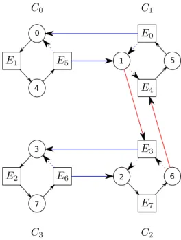
right part those from V2to V1. Figure 1 gives the representation digraph of the
de Bruijn dihypergraph GBH(2, 9, 2, 9) (see Section5), where vertex i belongs to the in-set of the hyperarcs E2i and E2i+1 and the hyperarc Ej has as out-set
the vertices 2j and 2j + 1 (all the numbers being taken modulo 9).
1 2 3 4 5 6 7 8 0 1 2 3 4 5 6 7 8 0
Figure 1: Bipartite representation of the De Bruijn dihypergraph GBH(2, 9, 2, 9) and a complete Berge dicycle represented by dotted arcs (ver-tices are drawn twice to better represent all the arcs).
Remark that when you inverse the respective roles of V1(R) and V2(R) in
R(H), you intuitively exchange the role of the vertices with the role of the hyperarcs in H. This is an informal notion of the dual dihypergraph H∗. For-mally, the vertices of the dual dihypergraph H∗ are in bijection φv with the
H. Moreover, for every vertex v ∈ V(H) and every hyperarc E ∈ E (H), vertex e = φv(E) ∈ V(H∗) is in V−, where V = φE(v) ∈ E (H∗), if, and only if, v ∈ E+
and, similarly, e is in V+ if, and only if, v ∈ E−. It is important to notice that a hyperarc V ∈ E (H∗) may have an empty in-set (if d−H(v) = 0) or an empty out-set (if d+H(v) = 0).
The underlying multidigraph U (H) of a dihypergraph H has as vertex set V(U (H)) = V(H) and as arc set E(U (H)) that is the multiset of all ordered pairs (u, v) such that u ∈ E− and v ∈ E+, for every hyperarc E ∈ E (H). We emphasize that U (H) does not need to be simple: the number of arcs from u to v in U (H) is the number of hyperarcs E = (E−, E+) in H such that u ∈ E− and v ∈ E+. Observe that the underlying multidigraph of a given dihypergraph is unique. However, a given digraph D can be the underlying digraph of many dihypergraphs H.
2.2
Eulerian and Hamiltonian Dicycles in Dihypergraphs
By a dipath in a dihypergraph H, we mean a sequence P = v0, E0, . . . , vp−1, Ep−1, vp,
such that, for all i, j, we have vi ∈ V(H), Ej ∈ E(H), vi ∈ E−i for every
0 ≤ i ≤ p − 1, and vi ∈ Ei−1+ for every 1 ≤ i ≤ p. We also say that P is a
dipath of length p. Moreover, the dipath P is called a dicycle, or circuit, in H if, and only if, we have v0 = vp. Observe that each dicycle in a dihypergraph
H corresponds to a dicycle in its bipartite representation R(H). Note that we allow repetitions of vertices or hyperarcs and some authors prefer to use the word tour in this case.
In the same way, we can extend the digraph-theoretic notions of Eulerian dicycles and Hamiltonian dicycles to dihypergraphs:
Definition 1. Let H be a dihypergraph. We say that H is Eulerian (resp. H is Hamiltonian) if, and only if, there is a dicycle C in H such that every hyperarc of H (resp. every vertex of H) appears in C exactly once. We call C an Eulerian dicycle (resp. a Hamiltonian dicycle).
Our generalization of an Eulerian dicycle to dihypergraphs is close to the extension of an Euler tour to the undirected hypergraphs introduced in [4]. Definition 2 ([4]). Let Hu be an undirected hypergraph. A tour is a sequence
T = v0, E0, v1, . . . ,
vm−1, Em−1, v0 where, for all i, vi 6= vi+1 and vi and vi+1 are in the hyperedge
Ei(indices are taken modulo m). T is called an Euler tour when every hyperedge
of Hu appears exactly once in T . Hu is an Eulerian hypergraph if there exists
an Euler tour T in Hu.
Remark 1. An Eulerian dicycle in H (resp. a Hamiltonian dicycle in H) is a dicycle in R(H), such that each vertex of V2(R) (resp. of V1(R)) appears exactly
As a consequence, a necessary and sufficient condition for R(H) to be Hamil-tonian is that there is a dicycle C in H, such that C is simultaneously an Eulerian dicycle and a Hamiltonian dicycle in H. In reference to the undirected case [3], we call C a complete Berge dicycle:
Definition 3. Let H be a dihypergraph. A complete Berge dicycle in H is a dicycle C in H, such that C is both an Eulerian dicycle and a Hamiltonian dicycle in H.
3
General Results
In the following sections, we focus on Eulerian dihypergraphs. Recall that we assume that the studied dihypergraphs have no isolated vertex, and that n > 1 and m > 1.
3.1
Some conditions
First, we recall a well-known characterization of Eulerian digraphs:
Theorem 1 ([22]). Let D be a digraph. The following statements are equivalent: 1. D is Eulerian;
2. D is (strongly) connected and, for all vertex v ∈ V(D), d−(v) = d+(v); 3. D is (strongly) connected and it has a dicycle decomposition (i.e. its arcs
can be partitioned into arc-disjoint dicycles).
The digraph-theoretic notions of connectivity can be extended to dihyper-graphs [19]. We say that H is strongly (resp. weakly) connected if its underlying multidigraph U (H) is strongly (resp. weakly) connected. U (H) is weakly con-nected if its associated multigraph GU (H) (obtained by forgetting the
orienta-tion) is a connected multigraph (in Graph Theory this undirected graph is often called the underlying graph; we use here a different terminology as we already use the word underlying for the digraph associated to a dihypergraph). The digraph-theoretic notions of vertex-connectivity and arc-connectivity are also generalized by the dihypergraph-theoretic notions of vertex-connectivity and hyperarc-connectivity (see [19]). Unlike 1-arc connected digraphs, 1-hyperarc connected dihypergraphs are not always 1-vertex connected.
Remark that unlike an Eulerian digraph, an Eulerian dihypergraph does not need to be strongly connected. Indeed, let H be an Eulerian dihypergraph. If we add a new vertex x in H, such that x is incident to only one hyperarc E of H and d−(x) = 0, then the dihypergraph obtained is still Eulerian, but it is not strongly connected.
On the other hand, we have the following necessary condition:
Proposition 2. Let H be a dihypergraph. If H is Eulerian, then H is weakly connected.
Proof. Let GU (H) be the undirected associated multigraph to U (H). We want
to prove that GU (H) is connected. Note first that for all hyperarc E ∈ E (H),
vertices in the subset E−∪ E+ are in the same connected component in G U (H),
by the definition of U (H). Moreover, let E, F be any pair of distinct hyperarcs of H. Since there is an Eulerian dicycle in H, therefore, there exist u ∈ E+ and v ∈ F−, such that there is a dipath in H from u to v. Since there is a dipath from u to v in H, therefore there is a dipath P from u to v in U (H) and so a path between u and v in GU (H). Therefore, the subsets E−∪ E+ and
F−∪ F+are in the same connected component in G
U (H) too. Therefore, GU (H)
is connected.
Recall that a hypergraph is k-uniform if all its hyperedges have the same car-dinality k. It was proved in [4] that, if H is an Eulerian k-uniform hypergraph, then |Vodd(H)| ≤ (k − 2)m(H), where Vodd(H) is the set of all the vertices in
H with an odd degree and m(H) is the number of hyperedges in H. Using the same idea, we also prove a necessary condition for a dihypergraph H to be Eulerian.
Theorem 3. Let H be a dihypergraph. If H is Eulerian then: X
v∈V(H)
|d+(v) − d−(v)| ≤ X
E∈E(H)
(|E+| + |E−| − 2).
Proof. Let C = v0, E0, v1, . . . , vm−1, Em−1, v0 be an Eulerian dicycle in H. By
definition, a given vertex may appear many times in C, but every hyperarc appears exactly once in the dicycle C. Let us find the maximum number of occurences of a given vertex v in C. For all i 6= j we may have vi= vj, but we
are sure that Ei 6= Ej. So a vertex v can appear at most min (d+(v), d−(v))
times in C and, as a consequence, we have the following inequality: X
v∈V(H)
min (d+(v), d−(v)) ≥ m
Moreover, we know that: min (d+(v), d−(v)) = 1 2(d +(v) + d−(v) − |d+(v) − d−(v)|), X v∈V(H) d+(v) = X E∈E(H) |E−| and X v∈V(H) d−(v) = X E∈E(H) |E+|.
Therefore, the following inequalities hold: X v∈V(H) (d+(v) + d−(v) − |d+(v) − d−(v)|) ≥ 2m X E∈E(H) |E−| + X E∈E(H) |E+| − X v∈V(H) |d+(v) − d−(v)| ≥ X E∈E(H) 2 X v∈V(H) |d+(v) − d−(v)| ≤ X E∈E(H) [(|E+| − 1) + (|E−| − 1)]
For a digraph D, Theorem 3 is
the Euler’s condition presented in Theorem 1: for all v ∈ V(D), d+(v) = d−(v).
Theorem 3 is not a sufficient condition for a strongly connected dihypergraph H to be Eulerian: counter-examples are presented in Figure 2 and in Figure 3(b).
0 1 2 3 0 1 2 3 E F G E F G
Figure 2: A regular dihypergraph that is not Eulerian.
Another necessary condition was proposed by N. Cohen (private commu-nication), who transposed the search of an Eulerian dicycle into a Perfect Matching problem (see [3, 2]).
Let H be a dihypergraph. If there is a hyperarc E ∈ E (H) whose in-set (resp. whose out-set) is empty, then H cannot be Eulerian. Else, let ϕ : E (H) → V(H) × V(H) be any function such that, for all E, we have ϕ(E) ∈ E−× E+.
By replacing each hyperarc E by the arc ϕ(E) we get a digraph, denoted by Dϕ[H] = (V(H), ϕ(E (H))). Observe that Dϕ[H] is a subdigraph of U (H) and
it can have loops or multiple arcs.
Remark 2. A dihypergraph H is Eulerian if, and only if, there exists a function ϕ such that Dϕ[H] is an Eulerian digraph.
By Theorem 1, a necessary and sufficient condition for a digraph D to be Eulerian is that D is connected and, for every vertex v, d−(v) = d+(v). If D satisfies this degree constraint for every vertex, but is not necessarily connected, we call D a balanced digraph.
We will use the well-known Hall’s Theorem to prove a necessary and sufficient condition for the digraph Dϕ[H] to be balanced, for some ϕ.
Theorem 4 (see [3, 2]). Let G = (V1∪ V2, E ) be a bipartite graph such that
|V1| = |V2|. There is a perfect matching in B if, and only if, for every subset
S ⊂ V1, |Γ(S)| ≥ |S|, where Γ(S) denotes the set of vertices adjacent to some
vertex of S.
Definition 4. Let X be a subset of V(H). We denote by d+H(X) (shortly d+(X)) the number of hyperarcs E ∈ E (H) such that E−∩X 6= ∅ and by d−s,H(X) (shortly denoted d−s(X)) the number of hyperarcs E such that E+⊆ X.
Theorem 5. Let H be a dihypergraph. There exists a function ϕ such that Dϕ[H] is a balanced digraph if, and only if, for every subset X ⊆ V(H), we
have d−s(X) ≤ d+(X).
Proof. Let us assume there exists ϕ such that Dϕ[H] is a balanced digraph. For
every subset X ⊆ V(H), for every hyperarc E such that E+⊆ X, we necessarily have (u, v) = ϕ(E) ∈ V(H) × X. Since Dϕ[H] is balanced, hence there must
be some hyperarc F such that ϕ(F ) has vertex v as origin, that is v ∈ F−. So F−∩ X is not empty. Furthermore, we can associate to two distinct hyperarcs E two distinct hyperarcs F ; therefore d−s(X) ≤ d+(X).
Conversely, let us assume that for every subset X ⊆ V(H), d−s(X) ≤ d+(X). Consider the bipartite graph BP (H) = (V1(BP ) ∪ V2(BP ), E (BP ))
with V1(BP ) = {Ej+ : Ej ∈ E(H)}, V2(BP ) = {Ej− : Ej ∈ E(H)} and
E(BP ) = {Ej+Ej−0 : E + j ∩ E − j0 6= ∅}. Let S = {Ej+ 1, E + j2, . . . , E + j|S|} be a subset of V1(BP ) and X = |S| [ k=1 Ej+ k.
Observe that |Γ(S)| = d+(X). Since d−s(X) ≥ |S|, we conclude that |Γ(S)| ≥
|S|. Moreover, V1(BP ) and V2(BP ) have the same cardinality. By Theorem
4, there is a perfect matching M in BP (H). We now define a function ϕ as follows: for all edge Ei+Ej− of M , one can choose any vertex v ∈ Ei+∩ Ej− as the tail of ϕ(Ei) and the head of ϕ(Ej). Thus, we get a subdigraph Dϕ[H] that
is a balanced digraph.
Observe that we may define d−(X) and d+s(X) in the same way as d+(X)
and d−s(X). Thus, another formulation of Theorem 5 is: there exists ϕ such
that Dϕ[H] is a balanced digraph if, and only if, for every subset X ⊆ V(H)
d+s(X) ≤ d−(X).
By Theorem 5, deciding whether there exists ϕ such that Dϕ[H] is a balanced
digraph can be done in polynomial time. However, deciding whether there exists ϕ such that Dϕ[H] is strongly connected is an NP-complete problem [23].
3.2
Duality and Complexity
First, we show that the search of an Eulerian dicycle in H is equivalent to the search of a Hamiltonian dicycle in its dual:
Proposition 6. A dihypergraph H is Eulerian if, and only if, H∗ is Hamilto-nian.
Proof. For each dicycle C = v0, E0, v1, E1, . . . , vp, Ep, v0 of H one can find a
corresponding dicycle in H∗namely C∗= e0, V1, e1, . . . , ep, V0, e0and vice-versa.
Thus, C is an Eulerian dicycle in H (i.e. C contains each hyperarc of H exactly once) if, and only if, C∗ contains each vertex of H∗ exactly once, i.e. C∗ is a Hamiltonian dicycle of H∗.
As a direct consequence we can observe that, since (H∗)∗ = H, H is Hamil-tonian if, and only if, H∗ is Eulerian. Moreover, since deciding whether a
di(hyper)graph H is Hamiltonian is an NP-complete problem [1], the following result is not surprising:
Theorem 7. Deciding whether a dihypergraph H is Eulerian is NP-complete. Proof. Let C be a dipath. One can verify, in O(|E (H)|) operations, whether C is an Eulerian dicycle in H. Consequently, the problem is in N P . Since the dual H∗can be built in O(|E (H)| + |V(H)|)-time, we conclude the proof directly from Proposition 6 and the NP-completeness of deciding whether a digraph is Hamiltonian.
In order to check if a given dihypergraph is Hamiltonian, we will often use the following proposition:
Proposition 8. A dihypergraph H is Hamiltonian if, and only if, its underlying multidigraph U (H) is Hamiltonian.
Proof. By definition of U (H), any dicycle in H is a dicycle in U (H) with the same vertices, and reciprocally.
3.3
Line Dihypergraphs Properties
The line dihypergraph L(H) of a dihypergraph H has as vertices the dipaths of length 1 in H and as hyperarcs the dipaths of length 1 in H∗:
V(L(H)) = [ E∈E(H) {(uEv) | u ∈ E−, v ∈ E+}, E(L(H)) = [ v∈V(H) {(EvF ) | v ∈ E+∩ F−};
where the in-set and the out-set of hyperarc (EvF ) are (EvF )−= {(uEv) | u ∈ E−} and (EvF )+= {(vF w) | w ∈ F+}.
Particularly, when D is a digraph, L(D) is the line digraph of D (see [1]). The following results are used in the sequel:
Theorem 9 ([19]). Let H be a dihypergraph. Then, 1. the digraphs R(L(H)) and L2(R(H)) are isomorphic; 2. the digraphs U (L(H)) and L(U (H)) are isomorphic; 3. the digraphs (L(H))∗ and L(H∗) are isomorphic.
Recall that:
Theorem 10 ([24]). For a given digraph D, the line digraph L(D) is Hamilto-nian if, and only if, D is Eulerian.
This property is useful for some special families of digraphs, e.g. Kautz and de Bruijn digraphs, that are stable by line digraph operation [24]. By using induction, one can prove that every digraph of the family is Hamiltonian. It was shown in [19] that de Bruijn and Kautz dihypergraphs are also stable by line dihypergraph operation. So, it is natural to wonder whether this property can be generalized to dihypergraphs. However, we only get a weak generalization. Proposition 11. Let H be a dihypergraph. Then, L(H) is Hamiltonian if, and only if, U (H) is Eulerian.
Proof. By Proposition 8, the dihypergraph L(H) is Hamiltonian if, and only if, U (L(H)) is Hamiltonian. Moreover, U (L(H)) and L(U (H)) are isomorphic by Theorem 9. Finally, by Theorem 10 L(U (H)) is Hamiltonian if, and only if, U (H) is Eulerian.
We now show with two counter-examples that both implications of the cor-responding version of Theorem 10 to dihypergraphs do not hold. There exist dihypergraphs which are Eulerian such that their line dihypergraph is not Hamil-tonian and there also exist dihypergraphs that are not Eulerian such that their line dihypergraph is Hamiltonian.
0 1 2 3 0 1 2 3 E F E F 4 4 (a) H1 0 1 2 3 0 1 2 3 E F G E F G (b) H2
Figure 3: Counter-examples for extension of Theorem 10 to dihypergraphs. Consider the dihypergraph H1= (V(H1), E (H1)) whose bipartite
representa-tion digraph is depicted in Figure 3(a). Observe that 0, E, 2, F, 0 is an Eulerian dicycle in H1. But d+U (H
1)(1) = 4, that is different than d −
U (H1)(1) = 3. As a
consequence, U (H1) cannot be Eulerian, by Theorem 1.
On the other hand, the dihypergraph H2 = (V(H2), E (H2)), depicted in
Figure 3(b), is not Eulerian, but U (H) is Eulerian and so L(H) is Hamiltonian. Remark that H2 verifies the necessary condition of Theorem 3. Furthermore,
H2 is strongly connected. One may observe that its underlying multidigraph
U (H2) is Eulerian (it is even a 2-regular digraph). However, H2is not Eulerian
because it does not verify the condition of Theorem 5. Indeed, d−s({1, 2}) = 2, which is strictly greater than d+({1, 2}) = 1.
We will show, in the next sections, that there are Eulerian dihypergraphs H, which are not digraphs, such that their U (H) is Eulerian.
4
Case of d-regular, s-uniform Dihypergraphs
Let (s−, s+) be a couple of positive integers. An (s−, s+)-uniform dihypergraph H is a dihypergraph such that the in-size (resp. the out-size) of every hyperarc in H equals s− (resp. equals s+). When s− = s+ = s we also say that H is a s-uniform dihypergraph. Recall that digraphs are 1-uniform dihypergraphs.
Let (d−, d+) be a couple of positive integers. A (d−, d+)-regular dihyper-graph H is a dihyperdihyper-graph such that the in-degree (resp. the out-degree) of every vertex in H equals d− (resp. d+). When d− = d+= d, we also say that H is a d-regular dihypergraph. Regular 1-uniform dihypergraphs are exactly regular digraphs. Remark that a dihypergraph H is (p, q)-uniform if, and only if, its dual dihypergraph H∗ is (p, q)-regular, for any positive integers p, q.
When the studied dihypergraphs are uniform, Theorem 3 can be reformu-lated in a very similar way to [4]:
Corollary 1. Let H be an Eulerian dihypergraph. If H is (s−, s+)-uniform, then:
X
v∈V(H)
|d+(v) − d−(v)| ≤ (s++ s−− 2) m
Observe that even though d-regular dihypergraphs always verify the neces-sary condition of Theorem 3, they are not always Eulerian (see Figure 2).
We recall the following result about regular digraphs:
Theorem 12 ([1]). Deciding whether a 2-regular digraph D is Hamiltonian is an NP-complete problem.
In [4], the authors use a similar result about 3-regular graphs, to prove that deciding whether a k-uniform hypergraph, k ≥ 3, is Eulerian is an NP-complete problem. We do the same for uniform dihypergraphs. First, observe that if the dihypergraphs are 1-uniform, that is they are digraphs, we know that deciding whether a digraph is Eulerian can be done in polynomial time [24].
Theorem 13. Let (s−, s+) be a couple of positive integers. If s− ≥ 2 or s+≥ 2,
then deciding whether a (s−, s+)-uniform dihypergraph is Eulerian is an NP-complete problem.
Proof. By symmetry, we only need to prove the case when s+≥ 2. Furthermore, by Theorem 7, we already know that the problem is in the NP-class. We now reduce the Hamiltonian problem in 2-regular digraphs to the Eulerian problem in (s−, s+)-uniform dihypergraphs.
The idea consists in associating in polynomial time to a 2-regular digraph D a dihypergraph HD, such that HD is Eulerian if, and only if, D is Hamiltonian
and then the result will follow by Theorem 12.
Let D = (V(D), E (D)) be a 2-regular digraph. We define the dihypergraph HD with the following rules:
1. V(HD) = V(D) ∪ {A × V(D)} ∪ {B × V(D)}, where A and B are two sets
2. to each vertex v ∈ V(D), we associate a hyperarc Ev ∈ E(HD) such that
Ev− = {v} ∪ {A × {v}} and Ev+ = {wv, w 0
v} ∪ {B × {v}}, where wv and
w0v are the out-neighbors of v in D.
By construction, HDis a (s−, s+)-uniform dihypergraph. Let us prove now that
D is Hamiltonian if, and only if, HD is Eulerian.
Suppose first that D is Hamiltonian and let C = v0, v1, . . . , vn−1, v0 be
a Hamiltonian dicycle in D. From C, we build a dicycle CD in HD, CD =
v0, Ev0, v1, Ev1, . . ., vn−1, Evn−1, v0, where Evi is the hyperarc that is induced
by vi. By definition of a Hamiltonian dicycle, for all v ∈ V(D), v appears only
once in C. Therefore, by construction of HD, for every Ev∈ E(HD), Evappears
exactly once in CD. So, CD is an Eulerian dicycle in HD.
Now, suppose that HDis Eulerian. Remark that for every E, F ∈ E (HD), by
construction of HD, we have E+∩F−⊂ V(D). Thus, let CD= v0, E0, v1, E1, . . . , vm−1, Em−1, v0
be an Eulerian dicycle in HD. Because of the previous remark, we know that for
every i, vi∈ V(D). However, a vertex v ∈ V(D) is incident to only one hyperarc
in HD. As a consequence, for all i, Ei is the hyperarc that is associated to vi
and so, each vi appears exactly once, and therefore, C = v0, v1, . . . , vm−1, v0 is
a Hamiltonian dicycle in D.
When H is a digraph, we know that:
Theorem 14 ([24]). Let D be a weakly-connected digraph. If D is regular, then all its iterated line digraphs Lk(D), for every k ≥ 1, are Hamiltonian and Eulerian.
We now prove that, more generally:
Theorem 15. Let H be a weakly-connected, d-regular, s-uniform dihypergraph. Then for every k ≥ 1, Lk(H) is Eulerian and Hamiltonian.
Proof. Since H is d-regular and s-uniform, then U (H) is a ds-regular multidi-graph. As a consequence, for all k ≥ 0, Lk(U (H)) is also ds-regular. By Theo-rem 9, we have by induction on k that, for all k ≥ 0, U (Lk(H)) is isomorphic to Lk(U (H)). So, for all k ≥ 0, U (Lk(H)) is Eulerian (because it is a regular multidigraph), that is equivalent, by Proposition 11, to L(Lk(H)) = Lk+1(H) be Hamiltonian.
Moreover, H∗ is s-regular, d-uniform, and we claim that it is also a weakly connected dihypergraph. Indeed, s ≥ 1 implies that there is no empty in-set and no empty out-set in H∗. So, the connectivity of H implies the connectivity of H∗. Therefore, for every k ≥ 1 Lk(H∗) is also Hamiltonian. Again by Theorem 9, we prove by induction on k that, for all k ≥ 1, (Lk(H))∗ is isomorphic to Lk(H∗). Therefore, by Proposition 6, for every k ≥ 1 Lk(H) is Eulerian. Remark 3. Theorem 15 holds when H is (d−, d+)-regular, H is (s−, s+ )-uniform, if we add the extra-condition: d−s−= d+s+.
Recall that a complete Berge dicycle is an Eulerian and Hamiltonian dicycle and that if a dihypergraph has such a dicycle, then its bipartite representation digraph R(H) is Hamiltonian. In the case s = d, we are able to prove a slightly more general result:
Proposition 16. Let H be a d-regular, d-uniform dihypergraph that is weakly connected. There is a complete Berge dicycle in L(H).
Proof. Because of the d-regularity, d-uniformity of H, its own bipartite repre-sentation digraph R(H) is d-regular. Therefore, for every i ≥ 1, Li(R(H)) is Hamiltonian. By Theorem 9, we know that L2(R(H)) and R(L(H)) are isomor-phic. Therefore, R(L(H)) is Hamiltonian.
Other results about Eulerian and Hamiltonian dihypergraphs can be found in [25].
5
de Bruijn and Kautz Dihypergraphs
In this section, we study the Eulerian and Hamiltonian properties of the gener-alization of de Bruijn and Kautz digraphs to dihypergraphs.
5.1
de Bruijn, Kautz and Consecutive-d digraphs
First, we recall some definitions and previous results on digraphs that we will use in the sequel.
Definition 5 ([14, 15]). The generalized de Bruijn digraph GB(d, n) (also called Reddy-Pradhan-Khul digraph), is the digraph whose vertices are labeled with the integers modulo n; there is an arc from vertex i to vertex j if, and only if, j ≡ di + α (mod n), for every α with 0 ≤ α ≤ d − 1.
If n = dD, GB(d, n) is nothing else than the de Bruijn digraph B(d, D) (see [13, 24]).
Definition 6 ([14]). The generalized Kautz digraph GK(d, n) (also called Imase-Itoh digraph), is the digraph whose vertices are labeled with the inte-gers modulo n; there is an arc from vertex i to vertex j if, and only if, j ≡ −di − d + α (mod n), for every α with 0 ≤ α ≤ d − 1.
If n = dD+ dD−1, GK(d, n) is nothing else than the Kautz digraph K(d, D) (see [13, 24]).
Both of those families of digraphs can be generalized in the following way: Definition 7 ([26]). Let 1 ≤ d, q ≤ n − 1, and 0 ≤ r ≤ n − 1, then the Consecutive-d digraph G(d, n, q, r) is the digraph whose vertices are labeled with the integers modulo n, such that there is an arc from vertex i to vertex j if, and only if, j ≡ qi + r + α (mod n), for every α with 0 ≤ α ≤ d − 1.
Observe that if q = d and r = 0, then G(d, n, d, 0) = GB(d, n) and that if q = r = n − d, then G(d, n, n − d, n − d) = GK(d, n).
Definition 8 ([27]). Let λ be a positive integer, with 1 ≤ λ ≤ d. Then GBλ(d, n) is the subdigraph of GB(d, n) such that there is a link from i to j
if, and only if, j ≡ di + α (mod n), for every 0 ≤ α ≤ λ − 1.
Actually, the digraph GBλ(d, n) is nothing else than the Consecutive-d
di-graph G(λ, n, d, 0). But the notation of GBλ(d, n) helps to understand that it
is a subdigraph of GB(d, n). If λ = d, GBd(d, n) = GB(d, n). We can define in
a similar way GKλ(d, n).
Consecutive-d digraphs have been intensively studied (see [26, 28, 29, 30, 31, 32, 33, 34, 35]). Particularly, the characterization of the Hamiltonian Consecutive-d Consecutive-digraphs is nearly complete:
Theorem 17 ([31, 26, 28, 29]). Let G = G(d, n, q, r) be a Consecutive-d digraph. • If d = 1, then G is Hamiltonian if, and only if, all of the four following
conditions hold: 1. gcd (n, q) = 1;
2. for every prime number p such that p divides n, then we have p divides (q − 1);
3. if 4 divides n, then 4 also divides (q − 1); 4. gcd (n, q − 1, r) = 1.
• If d = 2, then G is Hamiltonian if, and only if, one of the following conditions is verified:
1. gcd (n, q) = 2;
2. gcd (n, q) = 1 and either G(1, n, q, r) or G(1, n, q, r + 1) is Hamilto-nian.
• If d = 3, then:
1. if gcd (n, q) ≥ 2, G is Hamiltonian if, and only if, gcd (n, q) ≤ 3; 2. if gcd (n, q) = 1 and 1 ≤ |q| ≤ 3, G is Hamiltonian.
• If d ≥ 4, then G is Hamiltonian if, and only if, gcd (n, q) ≤ d.
Corollary 2 ([28]). Let G = G(d, n, q, r) be a Consecutive-d digraph. If gcd (n, q) ≥ 2, then G is Hamiltonian if, and only if, gcd (n, q) ≤ d.
The only remaining case is when d = 3, for which there is only a partial characterization.
In particular, the characterization of the Hamiltonian generalized de Bruijn (resp. Kautz) digraphs is complete:
Theorem 18 ([27]). If λ = gcd (n, d) ≥ 2, then GBλ(d, n) and GKλ(d, n) are
Hamiltonian.
Theorem 19 ([28, 27]). GB(d, n) is Hamiltonian if, and only if, one of the following conditions holds:
1. d ≥ 3;
2. d = 2 and n is even.
Theorem 20 ([28, 27]). GK(d, n) is Hamiltonian if, and only if, one of the following conditions holds:
1. d ≥ 3;
2. d = 2 and n is even;
3. d = 2 and n is a power of 3.
GB(d, n) and GK(d, n) are also Eulerian [27].
Finally, GB(d, n) and GK(d, n) have interesting line digraph properties. We use the following relations:
Proposition 21 ([27]). If gcd (n, d) = λ ≥ 2, then L(GBλ(d, n λ)) = GBλ(d, n) and L(GKλ(d, n λ)) = GKλ(d, n) Particularly: L(GB(d, n)) = GB(d, dn) and L(GK(d, n)) = GK(d, dn).
5.2
Definitions of de Bruijn and Kautz dihypergraphs
We now give the arithmetical definition for the de Bruijn and Kautz dihyper-graphs. For other definitions, see [12]. In what follows, the vertices (resp. the hyperarcs) are labeled with the integers modulo n (resp. modulo m); the ver-tices are denoted i, 0 ≤ i ≤ n − 1 and the hyperarcs Ej, 0 ≤ j ≤ m − 1. To
ease the reading we do not write, when it is clear in the context, the expressions (mod n) and (mod m).
Definition 9 ([12]). Let d, n, s and m be four positive integers, such that dn ≡ 0 (mod m) and sm ≡ 0 (mod n). The generalized de Bruijn dihypergraph GBH(d, n, s, m) has as vertex set (resp. hyperarc set) the integers modulo n (resp. modulo m). Any vertex i belongs to the in-set of hyperarcs Edi+α (mod m),
for every 0 ≤ α ≤ d − 1. Any hyperarc Ej has as out-set the vertices sj + β
(mod n), for every 0 ≤ β ≤ s − 1.
Note that the condition dn ≡ 0 (mod m) follows from the fact that the vertices i and i+n should be incident to the same hyperarcs d(i+n)+α ≡ di+α (mod m). Similarly Ej+= Ej+m+ implies sm ≡ 0 (mod n).
Particularly, when n = m, it can be useful to remark that in the bipartite digraph R(GBH(d, n, s, n)), the incidence relations from V1to V2 are the same
as in GB(d, n) and the incidence relations from V2 to V1 are the same as in
GB(s, n).
Definition 10 ([12]). Let (d, n, s, m) be four positive integers, such that dn ≡ 0 (mod m) and sm ≡ 0 (mod n). The generalized Kautz dihypergraph, denoted by GKH(d, n, s, m), is the dihypergraph whose vertices (resp. hyperarcs) are labeled by the integers modulo n (resp. modulo m), such that a vertex i is incident to hyperarcs Edi+α (mod m), for every 0 ≤ α ≤ d − 1 and hyperarc Ej
has for out-set the vertices −sj − s + β (mod n), for every 0 ≤ β ≤ s − 1. By inversing the labeling of the hyperarcs, it has been proposed in [12] an equivalent definition for Kautz dihypergraphs:
Definition 11 ([12]). Let (d, n, s, m) be four positive integers, such that dn ≡ 0 (mod m) and sm ≡ 0 (mod n). The generalized Kautz dihypergraph, denoted by GKH(d, n, s, m), is the dihypergraph whose vertices (resp. hyperarcs) are labeled by the integers modulo n (resp. modulo m), such that a vertex i is incident to hyperarcs E−di−d+α (mod m), for every 0 ≤ α ≤ d − 1 and hyperarc Ej has for
out-set the vertices sj + β (mod n), for every 0 ≤ β ≤ s − 1. We recall some properties that will be used in Section 6.
Theorem 22 ([12]). The underlying multidigraph of GBH(d, n, s, m) (resp. GKH(d, n, s, m)) is GB(ds, n) (resp. GK(ds, n)).
Theorem 23 ([12]). If H = GBH(d, n, s, m) (resp. GKH(d, n, s, m)), then H∗= GBH(s, m, d, n) (resp. GKH(s, m, d, n)).
Theorem 24 ([19]). The line dihypergraph of GBH(d, n, s, m) (resp. of GKH(d, n, s, m)) is GBH(d, dsn, s, dsm) (resp. is GKH(d, dsn, s, dsm)).
5.3
Eulerian and Hamiltonian properties
We now characterize when the generalized de Bruijn and Kautz dihypergraphs are Hamiltonian and Eulerian. Recall that we suppose n > 1 and m > 1. Theorem 25. Let H = GBH(d, n, s, m) be a generalized de Bruijn dihyper-graph. H is Hamiltonian if, and only if, one of the following conditions is verified:
1. ds ≥ 3;
2. ds = 2 and n is even.
Proof. First, recall that U (H) = GB(ds, n) by Theorem 22. By Theorem 19, we know that the de Bruijn digraph GB(ds, n) is Hamiltonian if, and only if, ds ≥ 3; or ds = 2 and n is even. Therefore, by Proposition 8, Theorem 25 follows.
Theorem 26. Let H = GBH(d, n, s, m) be a generalized de Bruijn dihyper-graph. H is Eulerian if, and only if, one of the following conditions is verified:
1. ds ≥ 3;
2. ds = 2 and m is even.
Proof. By Theorem 23, H∗ = GBH(s, m, d, n). Theorem 25 gives a necessary and sufficient condition for H∗to be Hamiltonian. By Proposition 6, this is also a necessary and sufficient condition for H to be Eulerian.
The method that is used for deciding whether GBH(d, n, s, m) is Eulerian or Hamiltonian can be applied to Kautz dihypergraphs in the same way. By Theorem 20, we have necessary and sufficient conditions for a generalized Kautz digraph to be Hamiltonian. Consequently:
Theorem 27. Let H = GKH(d, n, s, m) be a generalized Kautz dihypergraph. 1. If ds ≥ 3, then H is Eulerian and Hamiltonian;
2. If ds = 2, then H is Eulerian (resp. Hamiltonian) if, and only if, m (resp. n) is even or a power of 3.
6
Existence of Complete Berge Dicycles
In this section, we want to determine when there exists a complete Berge dicycle in GBH(d, n, s, m), (i.e a Hamiltonian dicycle in its bipartite representation digraph).
A necessary condition for a dihypergraph H to have a complete Berge dicycle is that n = m. Otherwise, R(H) cannot be Hamiltonian. We prove that: Theorem 28. There is a complete Berge dicycle in GBH(d, n, s, n) if one of the following conditions is verified:
1. d ≥ 3 and s ≥ 3;
2. d = 2 and s ≥ 4, or s = 2 and d ≥ 4;
3. {d, s} = {2, 3} and either n is even or n is a multiple of 3;
4. d = s = 2 and n is even or n is a power of 3 (otherwise it does not exist); 5. d = 1 or s = 1 and GB(ds, n) is Hamiltonian (otherwise it does not exist). The only remaining case is when {d, s} = {2, 3} and n and 6 are relatively prime, for which we conjecture GBH(d, n, s, n) has a complete Berge dicycle: Conjecture 29. If {d, s} = {2, 3}, then there is a complete Berge dicycle in GBH(d, n, s, n).
We highlight the particular case when s = d, for which we have a complete characterization:
Theorem 30. There is a complete Berge dicycle in GBH(d, n, d, n) if, and only if, one of the following conditions is verified:
1. d ≥ 3;
2. d = 2 and n is an even number; 3. d = 2 and n is a power of 3.
Remark that, for d ≥ 2, these conditions are exactly the same as those im-plying that GK(d, n) is Hamiltonian (see Theorem 20). It would be interesting to see if there is a relationship between Theorems 20 and 30. We were able to find it only when n is odd (see Lemma 5 in Section 6.4).
The rest of this section is devoted to the proof of Theorems 28 and 30. In Section 6.1, we deal with the easy case d = 1. In Section 6.2, we show that Theorem 28 is true when gcd (n, d) ≥ 2 and gcd (n, s) ≥ 2 using a special product of digraphs and the notion of line digraphs. Then, in Section 6.3, we consider the opposite case, where gcd (n, d) = 1 or gcd (n, s) = 1, and solve all the cases except {d, s} = {2, 3}, d = s = 2 and d = s = 3. Section 6.4 contains the lemma which shows the relation with the generalized Kautz digraphs, and that the conditions of Theorem 30 are sufficient for d = s = 2 and n is a power of 3. In Section 6.5, by using the Euler’s function, we show that these conditions are also necessary for d = s = 2. Finally, in Section 6.6, we deal with the remaining case: d = s = 3 and gcd (n, 3) = 1 and we solve it using a link-interchange method.
6.1
Case d = 1
Lemma 1. If d = 1, then there is a complete Berge dicycle in GBH(1, n, s, n) if, and only if, the de Bruijn digraph GB(s, n) is Hamiltonian.
Proof. If d = 1, then every vertex i is only incident to hyperarc Ei. So we
may not distinguish the vertices from the hyperarcs and we get a digraph, the relations of incidence of which are the relations of incidence between hyperarcs and vertices in the original dihypergraph. Therefore, Lemma 1 follows.
By symmetry, observe that the case when s = 1 is also solved by Lemma 1.
6.2
Case gcd (n, d) ≥ 2 and gcd (n, s) ≥ 2
In this section, we completely solve the case when gcd (n, d) ≥ 2 and gcd (n, s) ≥ 2. The proof is involved; in the particular case d = s, it can be simplified by using other methods such as the concatenation of digraph dicycles [25].
Definition 12 ([36, 37]). Let L1, L2 be two digraphs with the same order n and
with V(L1) ∩ V(L2) = ∅ and let φ: V(L1) → V(L2) be a one-to-one mapping.
Then, L1⊗φL2 is the digraph L such that V(L) = V(L1) ∪ V(L2) and the set
of arcs E (L) is defined by exchanging the out-neighbors of u ∈ V(L1) with the
out-neighbors of φ(u) ∈ V(L2) and vice-versa. More precisely, if u2 = φ(u1),
and (u1, v1) is an arc of L1 and (u2, v2) is an arc of L2, then the arcs (u1, v2)
and (u2, v1) belong to E (L).
Observe that if L1is the generalized de Bruijn digraph GB(s, n), L2 is the
generalized de Bruijn digraph GB(d, n) and φ is the identity function, then L1⊗φL2 is the bipartite representation digraph R(GBH(d, n, s, n)).
It happens that even if L1 and L2 are both strongly connected, L1⊗φL2
may be disconnected. However, it was proven by Barth and Heydemann the following sufficient condition:
Lemma 2 ([36]). If L1 and L2 are strongly connected, and if there exist u1
and u2 such that φ(u1) = u2 and there is a loop (u1, u1) ∈ E (L1) and a loop
(u2, u2) ∈ E (L2), then L1⊗φL2 is strongly connected.
We now prove a useful lemma:
Lemma 3. For every i ∈ {1, 2}, let Di be an arbitrary digraph and Li =
L(Di) be its line digraph. If L1 and L2 have the same number of vertices and
φ : V(L1) → V(L2) is a one-to-one mapping, then L1⊗φ L2 is also a line
multidigraph L(D), such that V(D) = V(D1) ∪ V(D2) and the degree of a vertex
in D is the same as the degree of its corresponding vertex in D1 or D2.
Proof. The vertices of Li (i = 1, 2) are the arcs of Di and so they are of the
form (ui, vi), with ui, vi∈ V(Di). Let V(D) = V(D1) ∪ V(D2). For each (u1, v1)
of L1, if (u2, v2) = φ((u1, v1)) is its image by φ, we put in D the arcs (u1, v2)
and (u2, v1).
Now, consider the mapping ψ : V(L1⊗φL2) → V(L(D)) = E (D), defined as
follows: if (u1, v1) is a vertex of L1 and (u2, v2) = φ((u1, v1)) is the associated
vertex in L2, then ψ((u1, v1)) = (u1, v2) and ψ((u2, v2)) = (u2, v1). Observe
that ψ is a one-to-one mapping. To prove the lemma, it suffices to prove that ψ keeps the adjacency relation.
On one side, by definition of the product, the vertex (u1, v1) is joined in
L1⊗φ L2 to the out-neighbors of (u2, v2) in L2 that is to the vertices of the
form (v2, w2), with (v2, w2) an arc of D2. On the other side, in L(D), the vertex
(u1, v2) = ψ((u1, v1)) is joined to the vertices (v2, y1), where y1is such that there
exists x1 in D1 and w2 in D2, such that (x1, y1) is an arc of D1, φ((x1, y1)) =
(v2, w2) and (v2, w2) is an arc of D2. But, by definition, (v2, y1) = ψ((v2, w2)).
So, ψ((u1, v1)) is joined in L(D) to all the images by ψ of the out-neighbors of
(u1, v1) in L1⊗φL2 and then the adjacency relation is kept for the vertices of
L1. The proof is identical for the vertices of L2.
When s = d, we can prove a stronger result namely that GBλ(d, n) ⊗φ
GBλ(d, n) is the line digraph of GBλ(d,
n
λ) ⊗φGBλ(d, n λ) [25].
Remark 4. Note that, if L1 = L(D1) and L2 = L(D2) are Hamiltonian
di-graphs, then D1 and D2 are balanced and so, by Lemma 3, D is a balanced
digraph, i.e. every vertex of D has equal in-degree and out-degree. Lemmas 2 and 3 enable us to prove the following theorem:
Theorem 31. Let H = GBH(d, n, s, n) be a generalized de Bruijn dihyper-graph. If gcd (d, n) ≥ 2 and gcd (s, n) ≥ 2, then there is a complete Berge dicycle in H.
Proof. Let us show that R = R(GBH(d, n, s, n)) is a Hamiltonian digraph. We recall that R is isomorphic to GB(s, n) ⊗φGB(d, n), φ being the identity
function. So, for λ = gcd (d, n) and µ = gcd (s, n), the digraph GBµ(s, n) ⊗φ
GBλ(d, n) is isomorphic to a subdigraph of R. As, by Proposition 21, GBµ(s, n)
and GBλ(d, n) are two line digraphs, then, by Lemma 3, GBµ(s, n)⊗φGBλ(d, n)
is also a line digraph L(D). Moreover, since GBµ(s, n) and GBλ(d, n) are
also Hamiltonian digraphs, by Theorem 18, then D is a balanced digraph by Remark 4. Furthermore, both GBµ(s, n) and GBλ(d, n) are strongly connected
and those two digraphs have a common loop (0, 0). Consequently, by Lemma 2, GBµ(s, n) ⊗φGBλ(d, n) is strongly connected, hence D is strongly connected
too.
D is a balanced digraph that is strongly connected. In other words, D is an Eulerian digraph and so L(D) = GBµ(s, n) ⊗φGBλ(d, n) is a Hamiltonian
digraph.
6.3
Case n and d relatively prime, or n and s relatively
prime
In the next proofs, we consider a Hamiltonian dicycle in a Consecutive-d digraph as a circular permutation σ in Zn. If j is the vertex that follows i in the
Hamiltonian dicycle, then σ(i) = j; if k is the vertex that follows j in the same dicycle, then σ2(i) = k and so on.
Now we deal with the other case gcd (n, d) = 1 or gcd (n, s) = 1 and will prove that the Theorem 28 holds in most of the cases. The proof will rely on the following lemma:
Lemma 4. Let n and d be relatively prime. If the Consecutive-s digraph G(s, n, ds, 0) is Hamiltonian, then there is a complete Berge dicycle in GBH(d, n, s, n). Proof. Recall that in G(s, n, ds, 0) a vertex i is joined to the vertices j ≡ dsi + β (mod n), for every β with 0 ≤ β ≤ s − 1. Let 0, σ(0), σ2(0), . . . , σn−1(0), 0 be a Hamiltonian dicycle of G(s, n, ds, 0). We construct the following dicycle in GBH(d, n, s, n). Vertex i precedes the hyperarc Edi. Since gcd (n, d) = 1,
there-fore d is invertible in Zn and i → di is a bijection between vertices and
hyper-arcs. The dicycle 0, E0, σ(0), Edσ(0), . . . , σn−1(0), Edσn−1(0), 0 is then a complete
Berge dicycle in GBH(d, n, s, n); indeed the vertex σk+1(0) ≡ s(dσk(0)) + βk ≡
Theorem 32. Let H = GBH(d, n, s, n) be a generalized de Bruijn dihyper-graph such that d 6= 1 and s 6= 1. If n and d are relatively prime or n and s are relatively prime, then there is a complete Berge dicycle in H if one of the following conditions hold:
1. d ≥ 4 or s ≥ 4;
2. {d, s} = {2, 3} and n is even or n is a multiple of 3.
Proof. By Theorem 17, we know that G(s, n, ds, 0) is Hamiltonian if one of the following conditions hold:
• s ≥ 4 and gcd(n, ds) ≤ s;
• or {s = 3 and 2 ≤ gcd(n, 3d) ≤ 3}; • or {s = 2 and gcd(n, 2d) = 2}.
Furthermore, if n and d are relatively prime, we have:
gcd (n, ds) = gcd (n, s) ≤ s (1) and so, 2 ≤ gcd(n, 3d) ≤ 3 is equivalent to n multiple of 3 and gcd(n, 2d) = 2 is equivalent to n even.
By using these facts and Lemma 4 we get:
• Fact 1: if n and d are relatively prime, then there is a complete Berge dicycle in GBH(d, n, s, n) when s ≥ 4 or {s = 3 and n is a multiple of 3} or {s = 2 and n is even}.
• Fact 2: (obtained by exchanging d and s) if n and s are relatively prime, then there is a complete Berge dicycle in GBH(s, n, d, n), hence, there is also a complete Berge dicycle in the dual GBH(d, n, s, n), when d ≥ 4 or {d = 3 and n is a multiple of 3} or {d = 2 and n is even}.
Now, we can conclude as follows:
Let d ≥ 4. If n and s are relatively prime we conclude by using Fact 2. Otherwise gcd(n, s) ≥ 2 and n and d are relatively prime. The theorem is proved by using Fact 1 as either s ≥ 4; or s = 3, but then n is a multiple of 3, because gcd(n, s) ≥ 2; or s = 2 and gcd(n, s) ≥ 2 implies that n is a multiple of 2.
The case s ≥ 4 can be done similarly (by exchanging d and s, which corre-sponds to work in the dual).
Now let d = 3 and s = 2. If n is a multiple of d = 3, then by hypothesis n and s are relatively prime and we conclude by Fact 2. If n is a multiple of s = 2, then by hypothesis n and d are relatively prime and we conclude by Fact 1. The case d = 2 and s = 3 is done similarly by exchanging d and s.
6.4
Concatenation of dicycles and relation to generalized
Kautz digraphs
If n is an odd number, then Theorem 30 can be partly proven with a concate-nation of dicycles.
Lemma 5. If GK(d, n) is Hamiltonian and n is odd, then there is a complete Berge dicycle in GBH(d, n, d, n).
Proof. We use a variant for the definition of GBH(d, n, d, n). Indeed as noted in [38], if we label the hyperarc Ej with label En−1−j, we get the incidence
relations of GK(d, n). In other words, GBH(d, n, d, n) can be defined as follows: vertex i is incident to hyperarcs E−di−d+α (mod n), for every 0 ≤ α ≤ d − 1,
and hyperarc Ej has as out-set the vertices −dj − d + β (mod n), for every
0 ≤ β ≤ d − 1.
Now, by Theorem 20, there exists a Hamiltonian dicycle in the Kautz digraph GK(d, n) for n odd, and either d ≥ 3 or { d = 2 and n is a power of 3}; let it be 0, σ(0), σ2(0), . . . , σn−1(0), 0. Let C be the dicycle of GBH(d, n, d, n), where vertex i precedes hyperarc Eσ(i) and hyperarc Ej precedes vertex σ(j). So,
C = 0, Eσ(0), σ2(0), . . . , σ2h(0), Eσ2h+1(0), . . . , σn−2(0), Eσn−1(0), 0, where 0 ≤
h ≤ n − 1. As n is odd, the n vertices and also the n hyperarcs of the dicycle are all different. Therefore C is a complete Berge dicycle in GBH(d, n, d, n). Corollary 3. If n is odd and d ≥ 3, then there is a complete Berge dicycle C in GBH(d, n, d, n).
Corollary 4. If n is a power of 3 and d = 2, then there is a complete Berge dicycle C in GBH(2, n, 2, n).
In the same way, we can prove that, if GB(d, n) is Hamiltonian and n is odd, then there is a complete Berge dicycle in GBH(d, n, d, n). However, even if it would have given the result for GBH(d, n, d, n) with n odd and d ≥ 3, it would have not been enough to conclude for the case d = 2 and n a power of 3. In that case, the proof of Lemma 5 plus the fact that, by [28], σ : i → −2i − 1 is a Hamiltonian dicycle in GK(2, n), gives the following complete Berge dicycle C in GBH(2, n, 2, n) (by renaming the edges with the standard definition). In C, vertex i precedes the hyperarc E2i, and hyperarc Ej precedes the vertex 2j + 1.
Thus, C contains as consecutive vertices i and 4i + 1. Figure 1 shows the dicycle 0, E0, 1, E2, 5, E1, 3, E6, 4, E8, 8, E7, 6, E3, 7, E5, 2, E4, 0, that is obtained in this
way for n = 9 (with dotted red arcs).
6.5
Case d = s = 2
Theorem 31 and Corollary 4 show that there exists a complete Berge dicycle in GBH(2, n, 2, n) when n is even, or {n is odd and n is a power of 3}. We still have to prove there is no complete Berge dicycle in the remaining cases. For that, we need to use the Euler function, in the spirit of the proof of [28].
Definition 13. The Euler function, denoted by ϕ, associates to a positive inte-ger n, the number ϕ(n) of positive inteinte-gers that are lower than n and relatively prime to n.
The Euler function satisfies the following properties (the three first ones are immediate consequences of the definition and the fourth one is known as Euler’s theorem):
1. ϕ(1) = 1;
2. If p is a prime number and m ≥ 1, then ϕ(pm) = (p − 1)pm−1; 3. If a and b are relatively prime, then ϕ(ab) = ϕ(a)ϕ(b);
4. If a and b are relatively prime, then aϕ(b)≡ 1 (mod b).
Lemma 6. If n is odd, then there is a complete Berge dicycle in GBH(2, n, 2, n) if, and only if, n is a power of 3.
Proof. Let us suppose that there is a complete Berge dicycle C in GBH(2, n, 2, n). We distinguish two cases: either there exists a vertex i, such that i precedes in C the hyperarc E2iand we will show this holds for all the vertices; or any vertex
i precedes in C the hyperarc E2i+1. To prove this claim, consider that some
vertex i precedes E2i in C. Since gcd (2, n) = 1, we have that 2 is invertible in
Zn. Thus, i0 = i − 2−1 cannot precede E2i0+1, as 2i0+ 1 = 2i. So, i0 precedes
E2i0 too. Consequently, since 2−1 is a generator element of Zn, any vertex i
precedes in C the hyperarc E2i.
Similarly, we can prove that either every hyperarc Ej in C precedes the
vertex 2j, or every hyperarc Ej in C precedes the vertex 2j + 1. Therefore, if we
consider only the vertices of the dicycle C and we denote by σ(i) the successor of i in C, we have exactly four possibilities for σ, namely: σk(i) = 4i + k with
0 ≤ k ≤ 3.
Since 4 · 0 = 0, the solution k = 0 does not generate a complete Berge dicycle. Furthermore, if gcd (n, 3) = 1 the equation σk(i) ≡ i ⇐⇒ 4i + k ≡ i
⇐⇒ 3i ≡ −k, has always a solution for 1 ≤ k ≤ 3. Therefore, none of the other values of k works, when gcd (n, 3) = 1.
It remains to consider the case n = c3p, p ≥ 1 and gcd (3, c) = 1. By induction, we have that σhk(0) =
k(4h− 1)
3 (mod n).
Let ϕ be the Euler function; by Properties 2 and 3, ϕ(n) = ϕ(c)ϕ(3p) = 2ϕ(c)3p−1. Since gcd(n, 2) = 1, then, by Property 4, 2ϕ(n)≡ 1 (mod n). There-fore, 4ϕ(c)3p−1 ≡ 1 (mod n) and, since ϕ(c)3p−1 < n, σ
3 never generates a
complete Berge dicycle either.
Moreover, since 2 is invertible in Zn, then we also know that σ2 generates
a complete Berge dicycle if, and only if, this is also the case for solution σ1.
Actually, when we choose σ1, we choose σ2 in the dual, and reciprocally. So,
let us concentrate now on σ1. The equation σ1h(0) = σ h0
1 (0) is equivalent to
4h≡ 4h0 (mod 3n). Again, Property 4 of Euler’s function implies that 4ϕ(c)3p
1 (mod 3n). But the only value of c such that ϕ(c) = c is c = 1. Therefore, if n is not a power of 3, σ1 and σ2do not generate a complete Berge dicycle.
This proof for d = 2 and n odd could be shortened using the characterization of the Hamiltonian Consecutive-1 digraphs. Indeed, we prove there are only four possibilities for having a complete Berge dicycle in GBH(2, n, 2, n). In the orig-inal proof, we deal with them as applications σk of Zn, for 0 ≤ k ≤ 3. But these
four solutions are also equivalent to some Consecutive-1 digraphs. They cor-respond, respectively, to the relations of incidence in G(1, n, 4, 0), G(1, n, 4, 1), G(1, n, 4, 2) and G(1, n, 4, 3). Then, deciding whether one of these four solutions generate a complete Berge dicycle is the same thing as deciding whether one of these four Consecutive-1 digraphs is a Hamiltonian digraph. Furthermore, by Theorem 17, we know whether one of those digraphs is Hamiltonian, depending on the value of n. For all n, G(1, n, 4, 0) and G(1, n, 4, 3) are never Hamilto-nian. Moreover, G(1, n, 4, 1) and G(1, n, 4, 2) are Hamiltonian if, and only if, n is a power of 3. Since the Hamiltonicity of at least one of these digraphs is a necessary and sufficient condition for H = GBH(2, n, 2, n) to have a complete Berge dicycle, then there is a complete Berge dicycle in H if, and only if, n is a power of 3.
6.6
Case d = s = 3
To finish the proof, it remains to deal with the case n even, d = s = 3 and n and d relatively prime. Note that, for d = 3, we do not know when the Consecutive-3 digraph G(3, n, 9, 0) is Hamiltonian, and so, we cannot use the same proof as in Lemma 4. We will use a method, introduced in [28], that is different from the previous ones. This method enables us to merge two disjoint dicycles of R(H) into one dicycle.
Definition 14. Let C1, C2 be two dicycles, that are subdigraphs of the same
digraph D. A pair {x1, x2} with x1 ∈ C1 and x2∈ C2 is called an interchange
pair if the predecessor y1of x1 in C1 is incident to x2in D, and the predecessor
y2 of x2 in C2 is incident to x1 in D too.
If {x1, x2} is an interchange pair, then we can build a dicycle containing
all the vertices of C1∪ C2 by deleting (y1, x1) and (y2, x2) and adding the arcs
(y1, x2) and (y2, x1).
Lemma 7. If n is even and n and 3 are relatively prime, then there is a complete Berge dicycle in GBH(3, n, 3, n).
Proof. Let R be the bipartite representation digraph of GBH(3, n, 3, n). To every vertex i we associate the hyperarc E3i+1and, similarly, to every hyperarc
Ej we associate the vertex 3j + 1. Since gcd (n, 3) = 1, the digraph R is
partitioned into pairwise vertex-disjoint dicycles. If there is only one dicycle in this partition, we are done as it is Hamiltonian. Otherwise, we use interchange pairs to merge successively the dicycles till we have only one. But we have to be careful to do independent interchanges.
Figure 4 shows an example for the case n = 8, where we obtain the 4 dicycles: C0= (0, E1, 4, E5), C1= (1, E4, 5, E0), C2= (2, E7, 6, E3), C3= (3, E2, 7, E6). 1 5 0 4 3 7 2 6
Figure 4: An application of the link-interchange method to the de Bruijn dihy-pergraph GBH(3, 8, 3, 8).
We first claim that, if i and i + 1 belong to two disjoint dicycles C1 and C2,
then {i, i + 1} is an interchange pair. Indeed, let Ej be the predecessor of i in
C1 and Ej0 the predecessor of i + 1 in C2. By construction, 3j + 1 = i and
3j0+ 1 = i + 1. Consequently, 3j + 2 = i + 1 and so there is an arc from Ej to
i + 1. We also have 3j0 = i and so there is an arc from Ej0 to i. Therefore, the
claim is proved. For n = 8, {0, 1} is an interchange pair and we can merge C0
and C1by deleting the arcs (E5, 0) and (E0, 1) (in dashed blue in Figure 4) and
adding the arcs (E5, 1) and (E0, 0) (in blue).
Similarly, we have that if Ej and Ej+1 belong to two disjoint dicycles then
{Ej, Ej+1} is an interchange pair. We have to be careful not to use twice the
same vertex in an interchange pair, as the predecessor has changed when doing the first merging. Here we will use only some interchange pairs of the form {2i, 2i + 1} and {E2j+1, E2j+2}, which are pairwise independent because n is
even.
We proceed as follows: if there exists an i such that 2i and 2i + 1 belong to different dicycles we merge these dicycles using the interchange pair {2i, 2i + 1}. After at most n/2 merge operations, we get a set of disjoint dicycles such that, for all i, 2i and 2i + 1 belong to the same dicycle. In the example for n = 8, we merge C0and C1using the interchange pair {0, 1} and C2 and C3 using the
interchange pair {2, 3} (see Figure 4). We now have 2 dicycles.
Then, consider two vertices of the form 2i and 2(i + 3−1). Suppose that they belong to two different dicycles C1 and C2. The vertex 2i + 1, which is also in
C1 precedes the hyperarc E6i+4in C1 and the vertex 2(i + 3−1) precedes E6i+3
in C2. Moreover, we claim that {E6i+3, E6i+4} is an admissible interchange pair
that we can use to merge the two dicycles, because 6i + 3 is odd whereas n is even, and so, 6i + 3 (mod n) is odd. Finally, since 3 and n are relatively prime, 3−1is a generator element in Znand so we can consider successively the possible
i such that 2i and 2(i + 3−1) belong to two different dicycles and merge all the dicycles.
Observe that for the example in Figure 4, when n = 8, we have that 3−1= 3. We now use the construction for i = 0. Vertices 0 and 6 are in two different dicycles, and {E3, E4} is an admissible interchange pair. So we can merge the
two dicycles by deleting the arcs (6, E3) and (1, E0) (in dashed red in Figure 4)
and adding the arcs (1, E3) and (6, E4) (in red) to get the final complete Berge
dicycle C = 0, E1, 4, E5, 1, E3, 3, E2, 7, E6, 2, E7, 6, E4, 5, E0, 0.
6.7
Complete Berge dicycles in Kautz Dihypergraphs
The Kautz dihypergraph GKH(d, n, d, n) is close to the dihypergraph GBH(d, n, d, n), but the existence of complete Berge dicycles in it is much harder to prove due to its asymmetry. Indeed, the relations of incidence from its vertices to the hyperarcs are not the same as the relations of incidence from its hyperarcs to the vertices.
Nonetheless, we have been able to show the existence of complete Berge dicycles in GKH(d, n, d, n) for some particular values of (d, n). Remark that R(GKH(d, n, d, n)) is isomorphic to the bipartite digraph BD(d, n) (see [39]). The proof of the following theorem uses the same tools as for GBH(d, n, d, n) and can be found in [25]
Theorem 33. Let H = GKH(d, n, d, n) be a Kautz dihypergraph. There is a complete Berge dicycle in H if one of the following conditions is verified:
1. d ≥ 4;
2. d = 3 and n is even;
3. d = 2 and n is even or n is a power of 5 (otherwise it does not exist); 4. d = 1 and n ∈ {1, 2} (otherwise it does not exist).
We also have the following conjecture concerning complete Berge dicycles in GKH(d, n, d, n):
Conjecture 34. Let H = GKH(d, n, d, n) be a Kautz dihypergraph. If d ≥ 3, then there is a complete Berge dicycle in H.
7
Conclusions
In this paper, we showed that it is an NP-complete problem to decide whether a dihypergraph is Eulerian (or Hamiltonian). We presented a generalization of some results concerning Eulerian digraphs, in the case where the studied dihypergraphs are uniform and regular. Then, we studied the Eulerian and Hamiltonian properties of generalized de Bruijn and Kautz dihypergraphs.
We let as open questions Conjectures 29 and 34. It would also be nice to find a relationship between Theorems 20 and 30, since both have similar conditions and different implications.
References
[1] J. Bang-Jensen, G. Gutin, Digraphs: theory, algorithms and applications, Springer Verlag, 2010.
[2] J. Bondy, U. Murty, Graph Theory with applications, 2nd Edition, Vol. 290, MacMillan London, 2008.
[3] C. Berge, Graphs and hypergraphs, Vol. 6, North-Holland Pub. Co., 1973. [4] Z. Lonc, P. Naroski, On tours that contain all edges of a hypergraph, The
electronic journal of combinatorics 17 (R144) (2010) 1.
[5] J.-C. Bermond, Hamiltonian decompositions of graphs, directed graphs and hypergraphs, Ann. Discrete Math. 3 (1978) 21–28, pr´esent´e au Cambridge Combinatorial Conf., Advances in graph theory , Trinity College, Cam-bridge, England, 1977.
[6] P. Keevash, D. K¨uhn, R. Mycroft, D. Osthus, Loose Hamilton cycles in hypergraphs, Discrete Mathematics 311 (2011) 544–559.
[7] D. K¨uhn, R. Mycroft, D. Osthus, Hamilton l-cycles in uniform hypergraphs, J. Comb. Theory Ser. A 117 (2010) 910–927. doi:10.1016/j.jcta.2010.02.010. [8] E. Arkin, M. Held, J. S. B. Mitchell, S. Skiena, Hamilton triangulations for fast rendering, in: Proceedings of the Second Annual European Symposium on Algorithms, ESA ’94, Springer-Verlag, London, UK, 1994, pp. 36–47. [9] J. Bartholdi III, P. Goldsman, Multiresolution indexing of triangulated
irregular networks., IEEE Trans. Vis. Comput. Graph. 10 (2004) 484–495. [10] J. Bartholdi III, P. Goldsman, The vertex-adjacency dual of a triangulated irregular network has a Hamiltonian tour, Operations Research Letters 32 (2004) 304–308.
[11] A. Dudek, A.Frieze, A. Ruci´nski, Rainbow hamilton cycles in uniform hy-pergraphs, Electronic Journal of Combinatorics 19 (2012) P46.
[12] J.-C. Bermond, R. W. Dawes, F. Ergincan, De Bruijn and Kautz bus networks, Networks 30 (3) (1997) 205–218. doi:10.1002/(SICI)1097-0037(199710)30:3¡205::AID-NET5¿3.0.CO;2-P.
[13] J.-C. Bermond, C. Peyrat, De Bruijn and Kautz networks: a competitor for the hypercube?, in: F. Andr´e, J.-P. Verjus (Eds.), Proceedings of the 1st European Workshop on Hypercubes and Distributed Computers, Rennes, North Holland, 1989, pp. 279–293.
[14] M. Imase, M. Itoh, Design to minimize diameter on building-block network, IEEE Transactions Computers C-30 (1981) 439–442.
[15] S. Reddy, D. Pradhan, J. Kuhl, Directed graphs with minimal diameter and maximal connectivity, Tech. rep., Oakland University, School of Engi-neering (1980).
[16] D.-Z. Du, D. F. Hsu, F. K. Hwang, The Hamiltonian property of consecutive-d digraphs, Mathematical and Computer Modelling 17 (11) (1993) 61 – 63. doi:10.1016/0895-7177(93)90253-U.
[17] T. E. Stern, K. Bala, Multiwavelength Optical Networks: A Layered Ap-proach, Addison-Wesley Longman Publishing Co., Inc., Boston, MA, USA, 1999.
[18] J.-C. Bermond, F. Ergincan, Bus interconnection networks, Discrete Ap-plied Mathematics 68 (1996) 1–15.
[19] J.-C. Bermond, F. Ergincan, M. Syska, Quisquater Festschrift, Vol. 6805 of Lecture Notes in Computer Science, Springer-Verlag, Berlin Heidelberg, 2011, Ch. Line Directed Hypergraphs, pp. 25–34.
[20] D. Ferrero, C. Padr´o, Connectivity and fault-tolerance of hyperdigraphs, Discrete Applied Mathematics 117 (2002) 15–26.
[21] D. Ferrero, C. Padr´o, Partial line directed hypergraphs, Networks 39 (2002) 61–67.
[22] V. Batagelj, T. Pisanski, On partially directed Eulerian multigraphs, Publ. de l’Inst. Math. Soc. 25 (39) (1979) 16–24.
[23] J. Bang-Jensen, S. Thomass´e, Decompositions and orientations of hyper-graphs, Tech. Rep. 10, IMADA (2001).
[24] J. De Rumeur, Communications dans les r´eseaux de processeurs, Masson, 1994.
[25] G. Ducoffe, Eulerian and Hamiltonian directed hypergraphs, Research Re-port 7893, INRIA (2012).
[26] D.-Z. Du, D. Hsu, On Hamiltonian consecutive-d digraphs, Banach Center Publications 25 (1989) 47–55.
[27] D.-Z. Du, F. K. Hwang, Generalized de Bruijn digraphs, Networks 18 (1) (1988) 27–38. doi:10.1002/net.3230180105.
[28] D.-Z. Du, D. F. Hsu, F. K. Hwang, X. M. Zhang, The Hamiltonian property of generalized de Bruijn digraphs, Journal of Combinatorial Theory, Series B 52 (1) (1991) 1 – 8. doi:DOI: 10.1016/0095-8956(91)90084-W.
[29] F. K. Hwang, The Hamiltonian property of linear functions, Operations Research Letters 6 (3) (1987) 125 – 127. doi:10.1016/0167-6377(87)90024-1.
[30] G. Chang, F. Hwang, L.-D. Tong, The Hamiltonian property of the consecutive-3 digraph, Mathematical and Computer Modelling 25 (11) (1997) 83 – 88. doi:10.1016/S0895-7177(97)00086-1.
[31] G. Chang, F. Hwang, L.-D. Tong, The consecutive-4 digraphs are Hamil-tonian, J. Graph Theory 31 (1999) 1–6.
[32] D.-Z. Du, D. Hsu, D. J. Kleitman, Modification of consecutive-d digraphs., in: Interconnection Networks and Mapping and Scheduling Parallel Com-putations. Proceedings DIMACS workshop February, 1994 Rutgers Univer-sity, New Brunswick, NJ, USA, Providence, RI: American Mathematical Society, 1994, pp. 75–85.
[33] D.-Z. Du, D. Hsu, G. Peck, Connectivity of consecutive-d digraphs, Discrete Appl. Math. 37-38 (1992) 169–177. doi:10.1016/0166-218X(92)90131-S. [34] D.-Z. Du, D. Hsu, H. Ngo, G. Peck, On connectivity of
consecutive-d consecutive-digraphs, Discrete Math. 257 (2002) 371–384. doi:10.1016/S0012-365X(02)00436-3.
[35] F. Cao, D.-Z. Du, F. Hsu, L. Hwang, W. Wu, Super line-connectivity of consecutive-d digraphs, Discrete Mathematics 183 (1-3) (1998) 27 – 38. doi:DOI: 10.1016/S0012-365X(97)00079-4.
[36] D. Barth, M.-C. Heydemann, A new digraphs composition, Research re-port, LRI, Universit´e de Paris-Sud, Orsay, France (1995).
[37] D. Barth, M.-C. Heydemann, A new digraphs composition with appli-cations to de Bruijn and generalized de Bruijn digraphs, Discrete Ap-plied Mathematics 77 (2) (1996) 99 – 118. doi:DOI: 10.1016/S0166-218X(96)00130-8.
[38] D. Coudert, Algorithmique et optimisation de r´eseaux de communications optiques, Ph.D. thesis, Universit´e de Nice Sophia-Antipolis (UNSA) (de-cember 2001).
[39] J. G´omez, C. Padr´o, S. P´erennes, Large generalized cycles, Discrete Applied Mathematics 89 (1-3) (1998) 107 – 123.