HAL Id: cea-01540849
https://hal-cea.archives-ouvertes.fr/cea-01540849
Preprint submitted on 16 Jun 2017
HAL is a multi-disciplinary open access
archive for the deposit and dissemination of
sci-entific research documents, whether they are
pub-lished or not. The documents may come from
teaching and research institutions in France or
abroad, or from public or private research centers.
L’archive ouverte pluridisciplinaire HAL, est
destinée au dépôt et à la diffusion de documents
scientifiques de niveau recherche, publiés ou non,
émanant des établissements d’enseignement et de
recherche français ou étrangers, des laboratoires
publics ou privés.
giants
Isabel Colman, Daniel Huber, Timothy Bedding, James Kuszlewicz, Jie Yu,
Paul Beck, Yvonne Elsworth, Rafael García, Steven Kawaler, Savita Mathur,
et al.
To cite this version:
Isabel Colman, Daniel Huber, Timothy Bedding, James Kuszlewicz, Jie Yu, et al.. Evidence for
compact binary systems around Kepler red giants. 2017. �cea-01540849�
Evidence for compact binary systems around Kepler red
giants
Isabel L. Colman
1,2∗, Daniel Huber
1,2,3,4, Timothy R. Bedding
1,2, James S. Kuszlewicz
2,5,
Jie Yu
1,2, Paul G. Beck
6, Yvonne Elsworth
2,5, Rafael A. Garc´ıa
6, Steven D. Kawaler
7,
Savita Mathur
8, Dennis Stello
1,2,9, and Timothy R. White
21Sydney Institute for Astronomy, School of Physics, A28, University of Sydney, NSW, 2006, Australia
2Stellar Astrophysics Centre, Department of Physics and Astronomy, Aarhus University, Ny Munkegade 120, DK-8000 Aarhus C, Denmark 3Institute for Astronomy, University of Hawai’i, 2680 Woodlawn Drive, Honolulu, HI 96822, USA
4SETI Institute, 189 Bernardo Avenue, Mountain View, CA 94043, USA
5School of Physics and Astronomy, University of Birmingham, Edgbaston, Birmingham B15 2TT, UK
6Laboratoire AIM, CEA/DRF - CNRS - Univ. Paris Diderot - IRFU/SAp, Centre de Saclay, 91191 Gif-sur-Yvette Cedex, France 7Department of Physics and Astronomy, Iowa State University, Ames, IA 50011, USA
8Center for Extrasolar Planetary Systems, Space Science Institute, 4750 Walnut street Suite 205, Boulder, CO 80301, USA 9School of Physics, University of New South Wales, NSW 2052, Australia
Accepted –. Received –; in original form –
ABSTRACT
We present an analysis of 168 oscillating red giants from NASA’s Kepler mission that exhibit anomalous peaks in their Fourier amplitude spectra. These peaks result from ellipsoidal variations which are indicative of binary star systems, at frequencies such that the orbit of any stellar companion would be within the convective envelope of the red giant. Alternatively, the observed phenomenon may be due to a close binary orbiting a red giant in a triple system, or chance alignments of foreground or back-ground binary systems contaminating the target pixel aperture. We identify 87 stars in the sample as chance alignments using a combination of pixel Fourier analysis and difference imaging. We find that in the remaining 81 cases the anomalous peaks are
indistinguishable from the target star to within 4′′, suggesting a physical association.
We examine a Galaxia model of the Kepler field of view to estimate background star counts and find that it is highly unlikely that all targets can be explained by chance alignments. From this, we conclude that these stars may comprise a population of physically associated systems.
Key words: stars: oscillations (including pulsations), (stars:) binaries (including
multiple): close
1 INTRODUCTION
This paper sets out to solve a long-standing problem in the study of oscillating Kepler red giants. The analysis of red giants has been an area of rapid growth with the advent of data from the Kepler mission (Borucki et al. 2010). In particular, asteroseismology has allowed unprecedented in-sights into their core fusion (Bedding et al. 2011), internal rotation (Mosser et al. 2012; Beck et al. 2012), and inter-nal magnetic fields (Stello et al. 2016). Red giants have also contributed to the field of galactic archaeology, where the study of red giant populations is used to map the formation
history of the galaxy (Miglio et al. 2013; Casagrande et al. 2016).
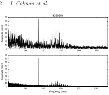
The red giants in this study were first noted in the early days of Kepler . Initial analysis revealed anomalous high-amplitude peaks in their Fourier spectra. Figure 1 shows amplitude spectra using the first quarter of data and data from all quarters for the first star observed to exhibit this behaviour, KIC 4350501 (Bedding et al. 2010). Note that the heights of the oscillation modes in the amplitude spec-trum decrease as the observing time is increased because the modes become more resolved.
These anomalous peaks were first suggested to be mixed modes (Bedding et al. 2010), which are caused by the cou-pling between p modes propagating in the convective
enve-50 100 150 200 250 0 10 20 30 40 50 60 70 80 A m p lit u d e (p p m ) 4350501 50 100 150 200 250 Frequency (µHz) 0 10 20 30 40 50 60 70 80 90 A m p lit u d e (p p m )
Figure 1. Top panel: Amplitude spectrum of KIC 4350501, the
first noted red giant with an anomalous peak, using only 43 days of data (Q0 and Q1), as in Bedding et al. (2010). Bottom panel: Amplitude spectrum calculated using all four years of Kepler data. The oscillations are centred at 140 µHz; the anomalous peak is at∼86 µHz.
lope with g modes propagating in the radiative core. Solar-like oscillations are stochastically excited and damped, with narrower peaks indicating longer mode lifetimes, as expected for mixed modes. For a recent review of red giants
and their oscillations, see Hekker & Christensen-Dalsgaard (2016). In the case of KIC 4350501, more data
showed the anomalous peak to be intrinsically narrow and revealed a subharmonic at half the frequency of the peak, suggesting that the peak was not a mixed mode but rather the signature of tidal interactions in a binary system. We have subsequently found many other red giants that show this type of behaviour, including the presence of harmonics and subharmonics. However, these peaks are present at such short periods that any binary companion would have to be orbiting within the convective envelope of the red giant.
This raises the possibility that we are observing common-envelope systems (Paczynski 1976). This is a phase of binary evolution that has been extensively studied with modelling and population synthesis. Evidence to confirm the existence of common-envelope systems is hard to come by; the closest method we have to direct detection is study-ing observational phenomena indicative of a past common-envelope phase. Recent studies have used the shaping of planetary nebulae with binary central stars to better un-derstand common-envelope interaction (Hillwig et al. 2016), and jets in planetary nebulae to constrain the magnetic fields of common-envelope binaries (Tocknell et al. 2014). It has also been postulated that the common-envelope phase could be integral to the evolution of red giants into sdB stars and cataclysmic variables (Beck et al. 2014). The observation of a common-envelope system would provide important confir-mation for these theories of binary evolution. For a recent review of our understanding of common-envelope systems, see Ivanova et al. (2013).
Another possibility is that these objects may be ex-amples of hierarchical triple systems, where a compact bi-nary orbits a red giant, e.g. “Trinity” (Derekas et al. 2011;
Fuller et al. 2013). These anomalous peaks could arise from a background or foreground compact binary that has con-taminated the light collected from the red giant. There is
still a limit to our knowledge of hierarchical triple systems and common-envelope binaries. The Trinity system is the best-studied observational example of a hierarchical triple involving a red giant. The red gi-ant in Trinity does not exhibit any oscillations, and it is expected that red giant oscillations would be suppressed by binarity, but we found no such trend in the stars in this study. Ultimately, we cannot ex-trapolate from the case of Trinity to the many pos-sible cases in this study, so the population of triple systems remains a hypothesis.
This study examines a sample of 168 light curves that exhibit both red giant oscillations and an anomalous peak, often with harmonics or a subharmonic. In this paper, we outline the method used to identify chance alignments, and comment on the statistics of possible physically associated systems.
2 METHODS AND ANALYSIS 2.1 Data preparation
The 168 stars studied were all discovered among Kepler red giants by visual inspection of power spectra. Many were in-cluded in Huber et al. (2010), Huber et al. (2011), or Stello et al. (2013). Additional stars were taken from Yu et al. (2016) or found in the APOKASC sample (Pinsonneault et al. 2014).
We began by downloading and preparing Kepler simple aperture photometry (SAP) light curves from MAST1. We
processed the light curves following Garc´ıa et al. (2011), initially performing a high-pass filter using a Gaussian of width 100 days. We followed this by clipping all outliers further than 3σ from the mean. Finally, we took a Fourier transform to produce the amplitude spectrum.
We first located the comb-like pattern of solar-like os-cillations, typical of red giant stars. Then, we were able to identify anomalous peaks. These have no particular posi-tion in relaposi-tion to the solar-like oscillaposi-tions. The majority of anomalous peaks had amplitudes higher than or compara-ble to the oscillations. Some anomalous peaks were found at similar frequencies to the oscillations, which led to a degree of confusion in stars that were identified previously with fewer quarters of data. A subset of the stars that we ini-tially considered to fit this pattern were discarded from this study due to the anomalous peak representing an oscillatory
ℓ = 0 or ℓ = 2 mode with a relatively broad peak, implying
a shorter mode lifetime.
Using the frequency of the high-amplitude anomalous peak, we phase-folded each star’s time series. The majority of the resulting phase curves displayed ellipsoidal variation, lending weight to the theory that these peaks are due to bi-narity. None of the anomalous peaks included in this study displayed the phase variation expected of a red giant oscil-lation. Examples are given in Figure 2. In some cases there were also subharmonics present in the Fourier spectra, as
0.0 0.5 1.0 1.5 2.0 Period: 0.30 days 0.99996 0.99998 1.00000 1.00002 1.00004 1.00006 1.00008 1.00010 1.00012 F ra c ti o n a l in te n s it y 6124426 0.0 0.5 1.0 1.5 2.0 Period: 0.40 days 0.9996 0.9998 1.0000 1.0002 1.0004 1.0006 6468112 0.0 0.5 1.0 1.5 2.0 Period: 0.70 days 0.9985 0.9990 0.9995 1.0000 1.0005 1.0010 6526377 0.0 0.5 1.0 1.5 2.0 Period: 0.68 days 0.9992 0.9994 0.9996 0.9998 1.0000 1.0002 1.0004 1.0006 11192141 0.0 0.5 1.0 1.5 2.0 Period: 0.26 days 0.9996 0.9997 0.9998 0.9999 1.0000 1.0001 1.0002 1.0003 F ra c ti o n a l in te n s it y 2018906 0.0 0.5 1.0 1.5 2.0 Period: 0.95 days 0.9998 0.9999 1.0000 1.0001 1.0002 4072864 0.0 0.5 1.0 1.5 2.0 Period: 0.48 days 0.99994 0.99996 0.99998 1.00000 1.00002 1.00004 1.00006 1.00008 1.00010 1.00012 5556726 0.0 0.5 1.0 1.5 2.0 Period: 0.57 days 1.00000 1.00002 1.00004 1.00006 1.00008 1.00010 1.00012 7198587
Figure 2. A variety of light curves phased on the period of the anomalous peak and binned. The top row shows stars that could not be
discounted as chance alignments in this study. The bottom row shows chance alignments.
15 20 25 30 35 40 0 50 100 150 200 250 300 350 A m p lit u d e (p p m ) 6707691 - γ-Dor 60 65 70 75 80 85 90 95 100 0 2 4 6 8 10 12 14 6707691 - RG 8 10 12 14 16 18 Frequency (µHz) 0 10 20 30 40 50 60 70 A m p lit u d e (p p m ) 9771905 - RG 160 180 200 220 240 260 280 Frequency (µHz) 0 50 100 150 200 250 300 9771905 - δ-Scuti
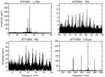
Figure 3. Top row: KIC 6707691, showing both γ-Dor (left) and red giant (right) oscillations. Bottom row: KIC 9771905, showing both red giant (left) and δ-Scuti (right) oscillations. Each set of oscillations is isolated to better display its features, as in each star the red giant oscillations have significantly lower amplitudes than the classical pulsator oscillations.
with KIC 4350501 (Figure 1), or a series of peaks indicative of an eclipse.
In two cases, we found the anomalous peaks to come from γ-Doradus oscillations and five stars where the source of the anomalous peaks are δ-Scuti pulsators, indicating possible binary systems. An ex-ample of red giants contaminated by γ-Dor and δ-Scuti oscillations is shown in Figure 3. Although these stars do not conform to the typical pattern of red giant oscillations with one anomalous peak and possible harmonics and subharmonics, we
in-clude them in this paper as they were studied with the same processes as the remainder of the sample and provide confirmation that the method works in-dependently of what type of target it is used to anal-yse.
2.2 Pixel power spectrum analysis
In the previous section we covered the process of identify-ing stars for this sample. For this, we used SAP light curves, which are a composite of several 4′′Kepler pixels comprising
the so-called ‘optimal aperture.’ To locate the true sources of these anomalous peaks, it was necessary to examine the area around each of the targets. For this, we used Kepler target pixel files (TPFs), which are available for download from MAST. TPFs provide a ‘postage stamp’ image of pixels around Kepler targets. We employed the same methods out-lined in Section 2.1 to process light curves from individual pixels in each TPF.
During the Kepler mission, the orientation of the tele-scope changed by 90◦every quarter. Because of this, we ex-amined each quarter of pixel data separately. In cases where oscillations were not visible with only one quarter of data, we stitched together the light curves of quarters with the same orientation, which occurred every fourth quarter.
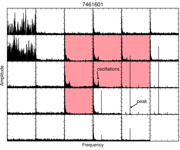
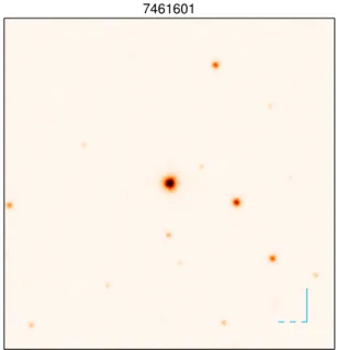
By taking a Fourier transform of each pixel time series, we could more accurately locate the source of the anomalous peaks in the Fourier spectra. We identified these by inspec-tion, based on the pixels included in the optimal aperture around the target star. In many cases, the source of the anomalous peak was obviously separated from the source of the solar-like oscillations. Figure 4 shows an example of such a TPF for KIC 7461601, where the optimal aperture is in-dicated by red shading. In this case, the anomalous peak is primarily located outside the optimal aperture. It is evident that its source is separate to the source of the oscillations. Of the 168 stars analysed, we found 87 to display this type
Frequency
A
m
p
lit
u
d
e
7461601
peak
oscillations
Figure 4. The Kepler TPF aperture of KIC 7461601, a red giant showing contamination from a chance alignment with a binary. Each panel represents a pixel, showing an amplitude spectrum calculated using the same methods as in Figure 1 with frequencies up to the Kepler long cadence Nyquist frequency, 283.21µHz. Amplitudes in each pixel are auto-scaled in order to better display qualitative features. More compact tick marks indicate higher overall amplitudes. Shaded pixels indicate the optimal aperture.
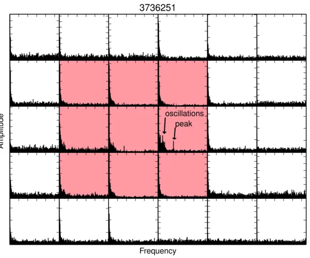
of clear separation. We interpret these as chance alignments of red giants with background or foreground binaries. The other 81 stars did not show this sort of clear separation. Fig-ure 5 shows the TPF for KIC 3736251, a case where there is no clear distinction between the pixel source of the red giant oscillations and the anomalous peak. We interpret these as possibly physically associated systems.
2.3 Difference imaging
We performed a more detailed study of the TPFs with dif-ference imaging, which has been successfully applied to the identification of false positive exoplanet transits (Bryson et al. 2013). We selected postage stamp images that fell in time within 10% bands centred on the maximum and mini-mum points of the phased light curve. To create the differ-ence image, we took the average of both sets of images and subtracted the average about the minima from the average about the maxima. This new image retained the dimensions of a TPF postage stamp and could easily be compared to the
average images, as shown in Figure 6. From this, we could see which pixels were the source of the flux variations at the period of the anomalous peak.
There remain some caveats for the use of difference imaging. The method we used was designed for ellipsoidal variation, and so it was less useful for the few stars in the sample where the phased light curve showed an eclipse, or where the identified anomalous peak belonged to δ-Scuti os-cillations with multiple high-amplitude peaks. There were several other issues with using the phased light curves, par-ticularly in stars with a low signal-to-noise ratio where the periodicity was hard to discern by looking at the phased light curve, due to scatter. Additionally, difference imaging was less successful for cases where the contaminant was at an angular distance greater than 30′′ from the target star. Some stars with clear contamination in the TPF did not show any variation in the difference image, which suggested that the contaminant was located outside the optimal aper-ture. This tended to coincide with low-amplitude anomalous
Frequency
A
m
p
lit
u
d
e
3736251
peak
oscillations
Figure 5. The Kepler TPF aperture of KIC 3736251, showing no contamination. Each panel represents a pixel, as in Figure 4.
Average Difference
Figure 6. An example of difference imaging, displaying the
KIC 7461601 aperture as in Figure 4. To indicate scale, the com-pass arms are 6′′. The solid line points north, and the dashed line points east. The variation originating from the bottom right corner of the TPF can be clearly seen in the difference image.
peaks. In such cases, it was clear simply from the TPFs that there was contamination.
Despite this, we were still able to gain valuable infor-mation from difference imaging. For stars with no evident contamination in the TPFs, the difference images tended not to show variation when compared to the average
im-ages. Difference imaging also helped to confirm the status of stars with low signal in the TPF Fourier spectra. Con-versely, the difference images reinforced the status of stars with more tentative classification as spatially separated. It follows that many of the cases where difference imaging did not confirm contamination correspond to widely separated chance alignments.
To identify the true source of chance alignments, widely-separated or otherwise, we next compared both the aver-age and difference imaver-ages to higher-resolution imaver-ages of the same area of sky, using 1′ cutouts from the UKIRT WF-CAM (the UK Infrared Telescope Wide Field Camera) sur-vey (Lawrence et al. 2007). An example is shown in Figure 7.
Kepler TPFs contain world coordinate system (WCS)
infor-mation, which allowed us to calculate the orientation of the postage stamp. We displayed coordinates on both types of images in the form of a compass rose, from which we could see whether there were any possible contaminant stars from the same position as the anomalous source as shown in the TPF Fourier spectra. Looking for matches in both the KIC and the UKIRT object catalogue, we were able to use a
Kepler light curve to confirm the source of contamination
7461601
Figure 7. A UKIRT image showing a 1′ field of view around KIC 7461601. To indicate scale, the compass arms are 6′′, as in Figure 6. The solid line points north, and the dashed line points east.
chance alignments (Table 4), we noted one or more possi-ble stars that could be the contaminant, especially closer to the Galactic plane, which is where most of the chance alignments were found.
3 DISCUSSION 3.1 Spatial distribution
We found that, of the 168 red giants with anomalous peaks, 87 could be identified as chance alignments. For 18 of these chance alignments, we confirmed their status with the anal-ysis of Kepler light curves of nearby stars which we identi-fied as the sources of contamination. We could not spatially resolve the 81 other stars, and we refer to these as possi-bly associated systems. We identified four of the five
δ-Scuti anomalous peaks as chance alignments. The
two γ-Dor anomalous peaks remain possible physical associations.
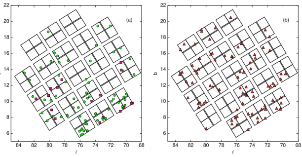
Figure 8 shows the distribution of our sample over the
Kepler field of view (FOV), with chance alignments in panel
(a) and possibly associated systems in panel (b). We present these populations in galactic coordinates, and note that the bottom of the field at lower galactic latitudes is closer to the Galactic plane and has a higher density of stars. At higher galactic latitudes we observe a marked paucity of stars as expected, both in the field itself and in the sample considered in this study. Similarly, this pattern presents itself in the distribution of chance alignments. It is therefore noteworthy that the possibly associated systems seen in panel (b) seem to be spread quite evenly across the FOV.
We further analysed these populations by examining
their cumulative distributions as a function of galactic lati-tude, shown in Figure 9. We compare this to a distribution of 1,000 red giants drawn randomly from a list of all oscillating
Kepler red giants provided from Yu et al. (in preparation).
The distribution of the possible physical associations closely matches the distribution of random red giants, which implies that they are not chance alignments. It is also noteworthy that these distributions visibly differ from the distribution of chance alignments, which increases sharply at low galactic latitudes, reflecting the higher density of stars closer to the Galactic plane. The probability of finding a chance align-ment between two populations is expected to scale as the square of surface density. This gives us an important insight into the nature of this population and suggests that we may be observing a distinct population of systems, possibly hi-erarchical triples or common envelope binaries.
3.2 Amplitude distribution
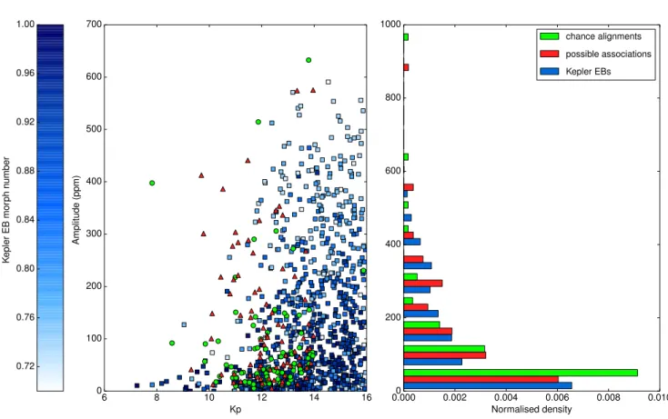
We searched for a possible correlation between the intrinsic luminosities of the red giants and the amplitudes of their anomalous peaks. It might be expected that if a compact binary is physically associated with a red giant, the ampli-tude of variations from the binary might correlate inversely with the luminosity of the red giant, due to dilution. We observed no correlation, which led us to compare our stars to a sample drawn from the Kepler Eclipsing Binary Cata-log (Prˇsa et al. 2011)2. We selected the sample of eclipsing binaries (EBs) by their morphology, which is a measure of the ellipticity of their phased light curves calculated by lo-cally linear embedding (Matijeviˇc et al. 2012). The cut off for EB selection was a morphology number > 0.7, chosen by visual inspection of stars in the catalog to match those with light curves similar to those in our sample. In Figure 10, we plot the amplitudes of the anomalous peaks in our sam-ple and of the Kesam-pler EBs against Kesam-pler magnitude. These data show that more ellipsoidal variation tends to have a lower amplitude of variation, a trend which is also present in our sample. The measure of ellipticity in our data was based on a ranking of the shape of phased light curves and on a different scale to the Catalog’s morphology number, so we do not display it in Figure 10.
From this exercise, we can explain the lack of correla-tion between the intrinsic luminosities of red giants and the amplitudes of their anomalous peaks by the broad range of amplitudes present across ellipsoidal variables, as exhibited by the Catalog sample. We also note that while our sample is overall brighter than the Catalog sample, the distribution of amplitudes is what would be expected for a sample pri-marily exhibiting ellipsoidal variation. The histogram in the right panel of Figure 10 shows that the distribution of the possible physical associations closely matches the distribu-tion of the Catalog EBs. The anomalous peaks of both the possible physical associations and the chance alignments are more present at lower amplitudes, but this is markedly no-ticeable for the latter. This effect can be explained by the wide angular separation between the target stars and their contaminants, so less of the contaminating light enters the
68 70 72 74 76 78 80 82 84 ℓ 6 8 10 12 14 16 18 20 22 b (a) 68 70 72 74 76 78 80 82 84 ℓ 6 8 10 12 14 16 18 20 22 b (b)
Figure 8. The sample of stars in this study is shown across the Kepler field of view in galactic coordinates. Panel (a) shows red giants
with anomalous peaks that we classified as chance alignments, shown as green circles. In the case where a Kepler light curve was available to confirm this contamination, the star is shown by a pink square. Panel (b) shows the population of red giants exhibiting an anomalous peak and where a physical separation cannot be discerned.
4 6 8 10 12 14 16 18 20 22 b 0.0 0.2 0.4 0.6 0.8 1.0 N o rm a lis e d d is tr ib u ti o n chance alignments (87) possible associations (81) Kepler red giants (1000)
Figure 9. Cumulative distributions in galactic latitude of the
populations shown in panels (a) and (b) of Figure 8. The solid blue line is taken from a random sample of 1,000 Kepler red giants.
optimal aperture. This leads to systematically lower aper-tures. In the case of the possible physical associations, this dilution could be caused by a compact binary companion. This strengthens the conclusion that the possible physical associations comprise a distinct population.
3.3 Modelling of chance alignments
While the majority of chance alignments found in this study involved contaminants further than 4′′from the target star,
it is possible that there could be contaminants within 4′′ of the target that our methods do not have the sensitivity to detect. To test whether we could expect to find more chance alignments within the remaining 81 stars, we anal-ysed a model of a stellar population in the Kepler FOV. This also helped us in understanding the underlying statis-tics around chance alignments of red giants and background or foreground binary systems.
We used the modelling software Galaxia (Sharma et al. 2011), which allows the user to synthesise an artificial pop-ulation of stars within a given area of sky, here chosen to match the Kepler FOV. We defined a chance alignment as any two stars found within a Kepler pixel of each other, namely 4′′. Galaxia does not take into account the existence of binary systems, and hence any chance alignments that are detected in the simulation are true chance alignments.
Our model goes down to an apparent J magnitude of 20. Once the synthetic FOV had been simulated, we then searched for stars analogous to those in the sample by min-imising over apparent J magnitude within a set range of galactic coordinates b and ℓ, and stellar parameters Teff,
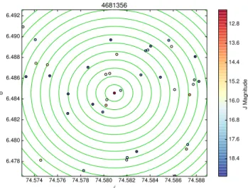
log(g) and [Fe/H] (Mathur et al. 2016). The nearest match to each target star was designated a blend if we located another star within 4′′ of it. This process is illustrated in Figure 11.
We found the occurrence of 4′′chance alignments in the model to be rare, with only 18 of 168 these stars fitting the criterion, or 10.7%. This is much lower than the observed fraction (as discussed in Section 3.1) because here we are only looking at matches within 4′′, which cannot be dis-cerned by the techniques covered in Section 2. This can be compared with the figure quoted in a study of false positive KOIs (Kepler Objects of Interest) by Ziegler et al. (2016), who found that planet host candidates have a nearby star
6 8 10 12 14 16 Kp 0 100 200 300 400 500 600 700 A m p lit u d e (p p m ) 0.000 0.002 0.004 0.006 0.008 0.010 Normalised density 0 200 400 600 800 1000 chance alignments possible associations Kepler EBs 0.72 0.76 0.80 0.84 0.88 0.92 0.96 1.00 K e p le r E B m o rp h n u m b e r
Figure 10. Left: Relationship between the amplitude of the anomalous peaks in our sample and Kepler magnitude. Chance alignments
are shown with green circles, and possible physical associations with red triangles. For comparison, we also display the amplitudes of a population selected from the Kepler Eclipsing Binary Catalog with morphology number > 0.7, shown with blue squares. Right: Histogram of each population distributed across amplitude. Not pictured: two outliers with amplitudes above 700ppm, one chance alignment (KIC 4071950) and one possible physical association (KIC 6526377).
within 0.15′′– 4′′with a probability of 12.6%± 0.9. Despite the fact that Ziegler et al. were not focused on red giants in the same way as our study, our value is just over 2σ from the result given by Ziegler et al., which places the two samples in good agreement. This suggests that a similar proportion of our sample will contain chance alignments within 4′′. By inspection of UKIRT images, 9 of the identified chance align-ments appear to be close to or within 4′′. This implies that we should expect to find roughly 9 more chance alignments within 4′′among the 81 stars that have not been identified as chance alignments. This is a strong result, and leaves us with a sizeable population of possible physical associations involving an oscillating red giant.
4 CONCLUSIONS
From a sample of 168 red giant stars with anomalous high-amplitude peaks, we found 87 could be discounted as chance alignments, with the remaining 81 exhibiting no contami-nation outside a Kepler pixel. This leaves the opportunity for these stars to be physically associated systems such as a common-envelope binary or hierarchical triple systems. We observe that this population appears to follow the dis-tribution of randomly-selected stars from the Kepler FOV. This distinguishes them from the population of chance align-ments, which appear with a greater density towards the
galactic plane. We have constructed and examined a model of a synthetic population in the Kepler field which suggests that such close chance alignments are rare, which would im-ply that most of these stars are more likely to be physically associated systems. This may point to hierarchical triple sys-tems, or to common-envelope binaries.
Future work includes an observation of all remaining targets by Robo-AO (Baranec et al. 2011), an adaptive optics system which has been used previously to examine
Kepler exoplanet host candidates. We will also look to
spec-troscopic follow-up observations, with the possibility of iden-tifying the spectral lines of companion stars or radial veloc-ity variations. In addition to this, further opportunities will arise to search for these unusual red giants in data from K2 and TESS. A larger sample from different areas of the sky would aid our understanding of these unusual cases and aid more detailed analysis of a possible new population of systems.
The fundamental parameters of the stars in this study are listed in tables in the appendix. All code used for anal-ysis is available online at https://github.com/astrobel/ chancealignments.
74.574 74.576 74.578 74.580 74.582 74.584 74.586 74.588 ℓ 6.478 6.480 6.482 6.484 6.486 6.488 6.490 6.492 b 4681356 12.8 13.6 14.4 15.2 16.0 16.8 17.6 18.4 J M a g n it u d e
Figure 11. An illustration of the process used to search for
chance alignments in the Galaxia model, described in Section 3.3. The concentric rings have radius 4′′, intended to represent the maximum distance between stars that could fall on the same
Kepler pixel. The colour scale represents J magnitude.
ACKNOWLEDGMENTS
This paper includes data collected by the Kepler mission. Funding for the Kepler mission is provided by the NASA Science Mission directorate. Some of the data presented in this paper were obtained from the Mikulski Archive for Space Telescopes (MAST). STScI is operated by the As-sociation of Universities for Research in Astronomy, Inc., under NASA contract NAS5-26555. Support for MAST for non-HST data is provided by the NASA Office of Space Sci-ence via grant NNX09AF08G and by other grants and con-tracts. The UKIDSS project is defined in Lawrence et al. (2007). UKIDSS uses the UKIRT Wide Field Camera (WF-CAM; Casali et al. (2007)) and a photometric system scribed in Hewett et al. (2006). The science archive is de-scribed in Hambly et al. (2008). We have used data from the 2nd data release, which is described in detail in War-ren et al. (2007). IC acknowledges scholarship support from the University of Sydney. DH acknowledges support by the Australian Research Council’s Discovery Projects fund-ing scheme (project number DE140101364) and support by the National Aeronautics and Space Administration under Grant NNX14AB92G issued through the Kepler Partici-pating Scientist Program. PGB, and RAG acknowledge the ANR (Agence Nationale de la Recherche, France) program IDEE (n◦ANR-12-BS05-0008) “Interaction Des Etoiles et des Exoplanetes”. PGB, and RAG also received funding from the CNES grants at CEA. YE acknowledges the sup-port of the UK Science and Technology Facilities Council (STFC). Funding for the Stellar Astrophysics Centre (SAC) is provided by The Danish National Research Foundation (Grant agreement no.: DNRF106). SM would like to ac-knowledge support from NASA grants NNX12AE17G and NNX15AF13G and NSF grant AST-1411685. DS is the re-cipient of an Australian Research Council Future Fellowship (project number FT1400147).
REFERENCES
Baranec C. et al., 2011, eprint: arXiv:1212.0825
Beck P. G. et al., 2014, Astronomy and Astrophysics, 564, A36
Beck P. G. et al., 2012, Nature, 481, 55
Bedding T. R. et al., 2010, The Astrophysical Journal Let-ters, 713, L176
Bedding T. R. et al., 2011, Nature, 471, 608 Borucki W. J. et al., 2010, Science, 327, 977
Bryson S. T. et al., 2013, Publications of the Astronomical Society of the Pacific, 125, 889
Casagrande L. et al., 2016, Monthly Notices of the Royal Astronomical Society, 455, 987
Casali M. et al., 2007, Astronomy and Astrophysics, 467, 777
Derekas A. et al., 2011, Science, 332, 216
Fuller J., Derekas A., Borkovits T., Huber D., Bedding T. R., Kiss L. L., 2013, Monthly Notices of the Royal Astronomical Society, 429, 2425
Garc´ıa R. A. et al., 2011, Monthly Notices of the Royal Astronomical Society, 414, L6
Hambly N. C. et al., 2008, Monthly Notices of the Royal Astronomical Society, 384, 637
Hekker S., Christensen-Dalsgaard J., 2016, ArXiv e-prints, 1609, arXiv:1609.07487
Hewett P. C., Warren S. J., Leggett S. K., Hodgkin S. T., 2006, Monthly Notices of the Royal Astronomical Society, 367, 454
Hillwig T., Jones D., De Marco O., Bond H., Margheim S., Frew D., 2016, ArXiv e-prints, 1609, arXiv:1609.02185 Huber D. et al., 2011, The Astrophysical Journal, 743, 143 Huber D. et al., 2010, The Astrophysical Journal, 723, 1607 Ivanova N. et al., 2013, Astronomy and Astrophysics
Re-view, 21, 59
Lawrence A. et al., 2007, Monthly Notices of the Royal Astronomical Society, 379, 1599
Mathur S. et al., 2016, ArXiv e-prints, 1609,
arXiv:1609.04128
Matijeviˇc G., Prˇsa A., Orosz J. A., Welsh W. F., Bloemen S., Barclay T., 2012, The Astronomical Journal, 143, 123 Miglio A. et al., 2013, Monthly Notices of the Royal
Astro-nomical Society, 429, 423
Mosser B. et al., 2012, Astronomy and Astrophysics, 548, A10
Paczynski B., 1976, in Structure and Evolution of Close Binary Systems; Proceedings of the Symposium, Vol. 73, D. Reidel Publishing Co., Cambridge, England, p. 75 Pinsonneault M. H. et al., 2014, The Astrophysical Journal
Supplement Series, 215, 19
Prˇsa A. et al., 2011, The Astronomical Journal, 141, 83 Sharma S., Bland-Hawthorn J., Johnston K. V., Binney J.,
2011, The Astrophysical Journal, 730, 3
Stello D., Cantiello M., Fuller J., Huber D., Garc´ıa R. A., Bedding T. R., Bildsten L., Aguirre V. S., 2016, Nature, 529, 364
Stello D. et al., 2013, The Astrophysical Journal Letters, 765, L41
Tocknell J., De Marco O., Wardle M., 2014, Monthly No-tices of the Royal Astronomical Society, 439, 2014 Warren S. J. et al., 2007, arXiv:astro-ph/0703037, arXiv:
Yu J., Huber D., Bedding T. R., Stello D., Murphy S. J., Xiang M., Bi S., Li T., 2016, Monthly Notices of the Royal Astronomical Society, 463, 1297
Ziegler C. et al., 2016, ArXiv e-prints, 1605,
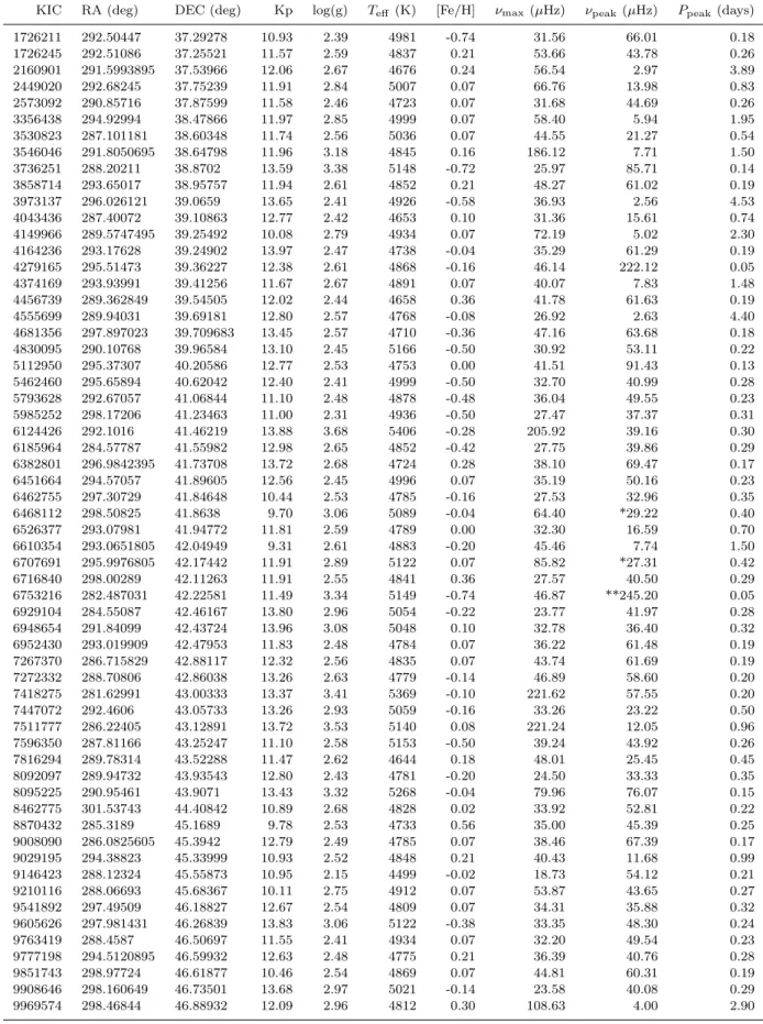
Table 1. Details of the 81 possible physical associations. Stellar parameters are taken from the NASA Exoplanet Archive, data release
25 (Mathur et al. 2016). In cases where we found the anomalous peak to be part of γ-Dor oscillations, the peak frequency (νpeak) is marked with an asterisk. We mark δ-Scuti anomalous peaks with two asterisks.
KIC RA (deg) DEC (deg) Kp log(g) Teff (K) [Fe/H] νmax (µHz) νpeak (µHz) Ppeak(days)
1726211 292.50447 37.29278 10.93 2.39 4981 -0.74 31.56 66.01 0.18 1726245 292.51086 37.25521 11.57 2.59 4837 0.21 53.66 43.78 0.26 2160901 291.5993895 37.53966 12.06 2.67 4676 0.24 56.54 2.97 3.89 2449020 292.68245 37.75239 11.91 2.84 5007 0.07 66.76 13.98 0.83 2573092 290.85716 37.87599 11.58 2.46 4723 0.07 31.68 44.69 0.26 3356438 294.92994 38.47866 11.97 2.85 4999 0.07 58.40 5.94 1.95 3530823 287.101181 38.60348 11.74 2.56 5036 0.07 44.55 21.27 0.54 3546046 291.8050695 38.64798 11.96 3.18 4845 0.16 186.12 7.71 1.50 3736251 288.20211 38.8702 13.59 3.38 5148 -0.72 25.97 85.71 0.14 3858714 293.65017 38.95757 11.94 2.61 4852 0.21 48.27 61.02 0.19 3973137 296.026121 39.0659 13.65 2.41 4926 -0.58 36.93 2.56 4.53 4043436 287.40072 39.10863 12.77 2.42 4653 0.10 31.36 15.61 0.74 4149966 289.5747495 39.25492 10.08 2.79 4934 0.07 72.19 5.02 2.30 4164236 293.17628 39.24902 13.97 2.47 4738 -0.04 35.29 61.29 0.19 4279165 295.51473 39.36227 12.38 2.61 4868 -0.16 46.14 222.12 0.05 4374169 293.93991 39.41256 11.67 2.67 4891 0.07 40.07 7.83 1.48 4456739 289.362849 39.54505 12.02 2.44 4658 0.36 41.78 61.63 0.19 4555699 289.94031 39.69181 12.80 2.57 4768 -0.08 26.92 2.63 4.40 4681356 297.897023 39.709683 13.45 2.57 4710 -0.36 47.16 63.68 0.18 4830095 290.10768 39.96584 13.10 2.45 5166 -0.50 30.92 53.11 0.22 5112950 295.37307 40.20586 12.77 2.53 4753 0.00 41.51 91.43 0.13 5462460 295.65894 40.62042 12.40 2.41 4999 -0.50 32.70 40.99 0.28 5793628 292.67057 41.06844 11.10 2.48 4878 -0.48 36.04 49.55 0.23 5985252 298.17206 41.23463 11.00 2.31 4936 -0.50 27.47 37.37 0.31 6124426 292.1016 41.46219 13.88 3.68 5406 -0.28 205.92 39.16 0.30 6185964 284.57787 41.55982 12.98 2.65 4852 -0.42 27.75 39.86 0.29 6382801 296.9842395 41.73708 13.72 2.68 4724 0.28 38.10 69.47 0.17 6451664 294.57057 41.89605 12.56 2.45 4996 0.07 35.19 50.16 0.23 6462755 297.30729 41.84648 10.44 2.53 4785 -0.16 27.53 32.96 0.35 6468112 298.50825 41.8638 9.70 3.06 5089 -0.04 64.40 *29.22 0.40 6526377 293.07981 41.94772 11.81 2.59 4789 0.00 32.30 16.59 0.70 6610354 293.0651805 42.04949 9.31 2.61 4883 -0.20 45.46 7.74 1.50 6707691 295.9976805 42.17442 11.91 2.89 5122 0.07 85.82 *27.31 0.42 6716840 298.00289 42.11263 11.91 2.55 4841 0.36 27.57 40.50 0.29 6753216 282.487031 42.22581 11.49 3.34 5149 -0.74 46.87 **245.20 0.05 6929104 284.55087 42.46167 13.80 2.96 5054 -0.22 23.77 41.97 0.28 6948654 291.84099 42.43724 13.96 3.08 5048 0.10 32.78 36.40 0.32 6952430 293.019909 42.47953 11.83 2.48 4784 0.07 36.22 61.48 0.19 7267370 286.715829 42.88117 12.32 2.56 4835 0.07 43.74 61.69 0.19 7272332 288.70806 42.86038 13.26 2.63 4779 -0.14 46.89 58.60 0.20 7418275 281.62991 43.00333 13.37 3.41 5369 -0.10 221.62 57.55 0.20 7447072 292.4606 43.05733 13.26 2.93 5059 -0.16 33.26 23.22 0.50 7511777 286.22405 43.12891 13.72 3.53 5140 0.08 221.24 12.05 0.96 7596350 287.81166 43.25247 11.10 2.58 5153 -0.50 39.24 43.92 0.26 7816294 289.78314 43.52288 11.47 2.62 4644 0.18 48.01 25.45 0.45 8092097 289.94732 43.93543 12.80 2.43 4781 -0.20 24.50 33.33 0.35 8095225 290.95461 43.9071 13.43 3.32 5268 -0.04 79.96 76.07 0.15 8462775 301.53743 44.40842 10.89 2.68 4828 0.02 33.92 52.81 0.22 8870432 285.3189 45.1689 9.78 2.53 4733 0.56 35.00 45.39 0.25 9008090 286.0825605 45.3942 12.79 2.49 4785 0.07 38.46 67.39 0.17 9029195 294.38823 45.33999 10.93 2.52 4848 0.21 40.43 11.68 0.99 9146423 288.12324 45.55873 10.95 2.15 4499 -0.02 18.73 54.12 0.21 9210116 288.06693 45.68367 10.11 2.75 4912 0.07 53.87 43.65 0.27 9541892 297.49509 46.18827 12.67 2.54 4809 0.07 34.31 35.88 0.32 9605626 297.981431 46.26839 13.83 3.06 5122 -0.38 33.35 48.30 0.24 9763419 288.4587 46.50697 11.55 2.41 4934 0.07 32.20 49.54 0.23 9777198 294.5120895 46.59932 12.63 2.48 4775 0.21 36.39 40.76 0.28 9851743 298.97724 46.61877 10.46 2.54 4869 0.07 44.81 60.31 0.19 9908646 298.160649 46.73501 13.68 2.97 5021 -0.14 23.58 40.08 0.29 9969574 298.46844 46.88932 12.09 2.96 4812 0.30 108.63 4.00 2.90
KIC RA (deg) DEC (deg) Kp log(g) Teff (K) [Fe/H] νmax(µHz) νpeak(µHz) Ppeak(days) 10334585 289.86435 47.43528 12.82 2.42 5023 -0.50 31.14 51.69 0.22 10384595 281.514071 47.50767 12.20 2.87 5186 0.07 44.83 55.09 0.21 10724041 288.92067 48.08529 12.28 2.41 4847 0.21 28.08 75.24 0.15 10855512 289.20384 48.20114 12.88 2.72 4724 0.00 65.23 12.09 0.96 10936814 298.47315 48.39799 10.79 2.47 4922 0.07 38.30 2.60 4.45 11140831 293.52471 48.79779 12.83 2.45 4862 -0.38 32.48 42.32 0.27 11145672 295.58421 48.79117 11.95 2.69 4915 -0.16 58.86 29.96 0.39 11177729 284.270741 48.87462 11.61 2.45 4896 0.07 32.84 42.99 0.27 11192141 292.719624 48.852017 10.52 2.01 4283 0.00 9.13 17.10 0.68 11287896 286.655441 49.03027 12.92 2.42 4947 0.07 34.53 55.10 0.21 11353223 293.29443 49.16571 12.47 2.63 4620 0.16 50.02 81.24 0.14 11400880 290.779849 49.27629 12.82 2.64 4755 -0.04 50.42 18.37 0.63 11567797 295.93539 49.51963 13.35 2.41 4816 0.07 30.69 5.60 2.07 11663151 292.58886 49.76146 11.96 2.68 4887 -0.24 36.30 47.11 0.25 11953849 285.76821 50.31719 11.20 2.45 4896 0.07 33.78 84.45 0.14 12003253 285.4657995 50.41648 11.19 2.41 4785 -0.24 34.27 4.48 2.58 12056767 288.59802 50.52476 10.14 2.45 4817 0.07 37.02 58.15 0.20 12067693 294.63153 50.55264 12.22 2.72 4862 0.36 29.97 65.34 0.18 12117920 295.27409 50.68874 12.18 2.45 4996 0.07 39.41 27.16 0.43 12645236 289.38545 51.76019 12.54 3.17 5114 -0.40 40.33 32.65 0.35 12737382 290.70515 51.90956 13.70 3.54 5023 -0.34 191.43 46.30 0.25
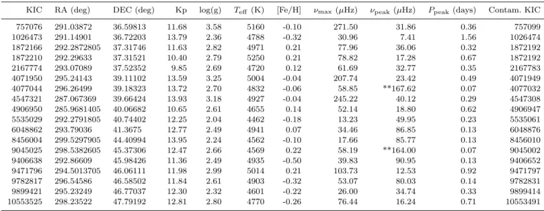
Table 2. Details of the 18 confirmed chance alignments with a known entry in the KIC. In cases where we found the anomalous peak
to be part of δ-Scuti oscillations, the peak frequency (νpeak) is marked with two asterisks.
KIC RA (deg) DEC (deg) Kp log(g) Teff (K) [Fe/H] νmax(µHz) νpeak (µHz) Ppeak (days) Contam. KIC
757076 291.03872 36.59813 11.68 3.58 5160 -0.10 271.50 31.86 0.36 757099 1026473 291.14901 36.72203 13.79 2.36 4788 -0.32 30.96 7.41 1.56 1026474 1872166 292.2872805 37.31746 11.63 2.82 4971 0.21 77.96 36.06 0.32 1872192 1872210 292.29633 37.31521 10.40 2.79 5250 0.21 78.82 17.28 0.67 1872192 2167774 293.07089 37.52352 9.85 2.69 4720 0.12 61.69 32.77 0.35 2167783 4071950 295.24143 39.11102 13.59 3.25 5004 -0.04 207.74 23.42 0.49 4071949 4077044 296.26499 39.18323 13.72 2.70 4832 -0.06 58.85 **167.62 0.07 4077032 4547321 287.067369 39.66424 13.93 3.18 4927 -0.04 245.22 40.12 0.29 4547308 4906950 285.9681405 40.06682 10.65 2.61 4655 0.14 52.14 18.80 0.62 4906947 5535029 292.2791805 40.74402 12.25 2.04 4462 -0.18 13.23 49.95 0.23 5535061 6048862 293.79036 41.3675 12.77 2.49 4941 0.07 34.46 86.85 0.13 6048876 8456004 299.5297905 44.40994 13.95 2.24 4562 -0.10 17.66 85.77 0.13 8456010 9045025 298.5382605 45.37306 12.47 2.66 4569 0.22 58.19 **164.00 0.07 9045002 9406638 292.86609 45.98426 11.36 2.49 4935 -0.50 39.83 90.95 0.13 9406652 9471796 294.5013705 46.06111 11.98 2.99 5014 0.21 103.73 12.53 0.92 9471797 9782817 296.54586 46.58502 11.84 2.61 4903 -0.32 53.07 80.03 0.14 9782831 9899421 295.23249 46.77037 12.30 2.32 4601 -0.22 26.00 34.74 0.33 9899414 10553525 298.23522 47.79192 12.81 2.80 4770 -0.26 76.44 16.24 0.71 10553491
Table 3. Details of the 69 presumed chance alignments. In cases where we found the anomalous peak to be part of δ-Scuti oscillations,
the peak frequency (νpeak) is marked with two asterisks.
KIC RA (deg) DEC (deg) log(g) Kp Teff (K) [Fe/H] νmax(µHz) νpeak (µHz) Ppeak (days)
1870196 291.8805 37.34748 12.65 3.20 4895 0.10 191.59 60.77 0.19 2018906 292.42326 37.428 13.20 3.30 5046 -0.54 155.70 44.07 0.26 2163856 292.22694 37.55744 11.70 2.78 5010 0.07 72.14 144.29 0.08 2301349 291.09195 37.64004 13.43 2.72 4615 0.36 64.62 33.95 0.34 2569650 290.19609 37.81097 15.88 3.62 4986 0.22 187.60 74.04 0.16 2569935 290.222441 37.80783 13.12 1.55 4082 0.36 5.21 71.10 0.16 2696115 286.8690795 37.95218 11.85 2.19 4619 0.21 20.41 42.07 0.28 2710194 290.79134 37.92911 12.15 2.68 4580 0.24 54.74 33.60 0.34
KIC RA (deg) DEC (deg) log(g) Kp Teff (K) [Fe/H] νmax(µHz) νpeak (µHz) Ppeak(days) 3118806 291.95328 38.21967 10.99 2.18 4569 0.36 18.05 57.58 0.20 3660820 295.19049 38.76184 11.87 2.40 4969 0.07 31.36 69.17 0.17 3858850 293.68329 38.98237 12.01 2.31 4523 0.36 20.33 83.69 0.14 3866844 295.5547695 38.99418 12.65 2.42 4710 0.36 33.33 64.32 0.18 3953330 291.242981 39.09661 12.55 2.28 4627 -0.44 16.58 6.30 1.84 3955590 291.86157 39.01267 10.34 2.19 4673 0.21 97.25 21.22 0.55 4059983 292.2911 39.10751 13.44 2.83 4842 0.56 31.96 51.18 0.23 4072864 295.445499 39.12097 13.81 3.34 4961 -0.06 183.22 12.17 0.95 4136374 284.8337805 39.21037 10.84 2.62 4876 0.07 48.53 7.32 1.58 4350501 287.07155 39.41622 11.74 3.06 5016 -0.22 141.40 86.65 0.13 4482738 296.13902 39.57963 12.95 3.06 4936 -0.44 141.34 53.44 0.22 4937770 295.47659 40.03605 13.15 2.90 4924 -0.32 91.11 63.60 0.18 4951617 298.4266905 40.06777 10.89 2.68 4822 0.04 43.31 110.44 0.10 5024414 295.316379 40.18652 12.71 2.81 5000 0.07 71.39 147.05 0.08 5112880 295.362821 40.20787 12.29 2.30 4501 0.10 27.71 66.38 0.17 5219666 299.3242695 40.37239 12.59 2.64 4665 0.36 56.52 29.74 0.39 5304555 298.761761 40.45563 12.78 2.56 4840 0.21 46.76 75.55 0.15 5308777 299.5773105 40.49851 13.20 2.84 4877 0.14 86.42 12.25 0.94 5385245 297.54492 40.55547 10.96 3.08 5083 -0.14 124.83 6.83 1.70 5556726 297.62054 40.76302 12.17 3.21 4898 0.07 207.26 24.04 0.48 5561523 298.632431 40.79503 13.47 2.99 4948 -0.06 34.49 73.03 0.16 5598645 283.7800305 40.81878 11.69 3.21 4973 -0.14 261.85 17.84 0.65 5648894 298.88994 40.82022 8.58 2.81 5068 -0.36 74.87 30.16 0.38 5725960 297.1535 40.92263 12.26 3.45 5171 -0.28 242.25 67.00 0.17 5736093 299.20563 40.91081 13.02 2.93 5121 0.07 106.57 50.05 0.23 6105113 284.81205 41.41103 13.24 3.10 4754 -0.02 32.89 52.65 0.22 6382830 296.992239 41.7899 11.01 2.24 4716 0.21 22.17 56.83 0.20 6447614 293.355371 41.88883 13.85 3.47 5132 -0.64 27.02 85.11 0.14 6612644 293.71154 42.01754 12.51 2.60 4681 0.28 44.85 18.77 0.62 6701238 294.48732 42.16711 11.30 2.40 4777 -0.30 27.26 97.46 0.12 6952355 292.99371 42.43124 13.11 2.98 4864 0.00 118.39 27.38 0.42 6963285 295.8375 42.49793 13.51 2.75 5102 0.21 181.09 57.55 0.20 7198587 291.2658405 42.73949 12.89 3.18 4968 0.18 168.98 20.42 0.57 7335713 280.902429 42.93572 12.44 3.13 5261 -0.56 155.32 40.35 0.29 7461601 296.29989 43.07131 13.43 2.90 4893 -0.46 50.17 82.46 0.14 7604896 290.9272605 43.23875 13.09 2.92 4878 0.06 99.38 72.13 0.16 7630743 297.9376695 43.28479 12.62 3.14 4786 0.07 166.91 86.71 0.13 7631194 298.05033 43.23317 11.82 2.68 4994 0.07 58.83 57.06 0.20 7831725 294.8964 43.52991 12.87 2.66 4985 0.07 39.10 35.81 0.32 7880664 287.7593895 43.68936 12.36 2.63 4802 0.07 39.26 99.11 0.12 7944142 284.869578 43.733161 7.82 2.80 5055 0.07 74.88 6.69 1.73 8052184 298.7172 43.85774 13.51 3.56 5196 -0.30 253.94 78.51 0.15 8409750 281.62728 44.41363 12.20 3.27 5245 -0.18 206.51 36.58 0.32 8649099 299.32878 44.79816 11.23 2.54 4845 -0.20 44.92 74.07 0.16 8914107 300.59514 45.15587 12.08 3.12 4910 -0.06 165.07 230.17 0.05 9091772 292.936899 45.41815 11.53 2.95 5026 0.07 115.53 48.25 0.24 9291830 295.97199 45.71479 11.02 2.56 5038 0.07 43.86 85.70 0.14 9479404 297.08928 46.03567 9.83 2.85 5191 0.21 77.41 10.02 1.16 9582089 289.24935 46.26023 12.22 2.45 4608 0.24 23.72 80.49 0.14 9612084 299.8694295 46.24609 11.76 3.05 5095 -0.06 78.60 **265.85 0.04 9771905 292.40451 46.5417 11.71 2.15 4393 0.16 11.47 **238.68 0.05 9906673 297.57587 46.76234 12.74 2.69 4937 -0.22 37.73 27.36 0.42 10203751 290.21211 47.202 11.96 2.58 4816 -0.08 35.69 13.18 0.88 10528911 289.28019 47.70018 12.06 2.39 4889 0.21 33.33 60.12 0.19 10854977 288.95117 48.22104 13.81 3.19 5193 -0.24 181.64 10.47 1.11 10858675 290.6682705 48.20462 12.24 2.84 4967 -0.08 87.12 24.31 0.48 10878851 298.14741 48.29483 13.21 2.44 4981 0.07 34.02 79.74 0.15 11298371 292.571829 49.03284 10.26 2.44 4989 0.07 35.28 59.76 0.19 11618859 295.67499 49.61104 13.77 3.64 5355 0.04 259.83 33.80 0.34 11753010 285.65682 49.90863 11.01 2.06 4303 0.14 14.03 89.70 0.13 12117138 294.895719 50.60238 12.50 2.53 4805 0.07 39.99 2.63 4.40