HAL Id: hal-00299471
https://hal.archives-ouvertes.fr/hal-00299471
Submitted on 28 Nov 2007
HAL is a multi-disciplinary open access
archive for the deposit and dissemination of
sci-entific research documents, whether they are
pub-lished or not. The documents may come from
teaching and research institutions in France or
abroad, or from public or private research centers.
L’archive ouverte pluridisciplinaire HAL, est
destinée au dépôt et à la diffusion de documents
scientifiques de niveau recherche, publiés ou non,
émanant des établissements d’enseignement et de
recherche français ou étrangers, des laboratoires
publics ou privés.
Ultrasound monitoring of applied forcing, material
ageing, and catastrophic yield of crustal structures
G. P. Gregori, M. Lupieri, G. Paparo, M. Poscolieri, G. Ventrice, A. Zanini
To cite this version:
G. P. Gregori, M. Lupieri, G. Paparo, M. Poscolieri, G. Ventrice, et al.. Ultrasound monitoring of
applied forcing, material ageing, and catastrophic yield of crustal structures. Natural Hazards and
Earth System Science, Copernicus Publications on behalf of the European Geosciences Union, 2007,
7 (6), pp.723-731. �hal-00299471�
www.nat-hazards-earth-syst-sci.net/7/723/2007/ © Author(s) 2007. This work is licensed under a Creative Commons License.
and Earth
System Sciences
Ultrasound monitoring of applied forcing, material ageing, and
catastrophic yield of crustal structures
G. P. Gregori1,2, M. Lupieri1,2, G. Paparo1,3, M. Poscolieri1,2, G. Ventrice4, and A. Zanini5
1Istituto di Acustica “O.M. Corbino”, C.N.R., Via Fosso del Cavaliere 100, 0133 Rome, Italy 2ICES – International Centre for Earth Sciences, Via Fosso del Cavaliere 100, 00133 Rome, Italy 3Italian Embassy, Buenos Aires, Argentina
4P.M.E. Engineering, Rome, Italy
5Alitalia, Power Plant Engineering Dept., Rome, Italy
Received: 20 July 2007 – Revised: 5 November 2007 – Accepted: 5 November 2007 – Published: 28 November 2007
Abstract. A new kind of data analysis is discussed – and
a few case histories of actual application are presented – concerning the physical information attainable by acoustic emission (AE) records in geodynamically active or volcanic areas. The previous analyses of such same kind of observa-tions were reported in several papers appeared in the last few years, and here briefly recalled. They are concerned with the inference of the forcing (“F ”) acting on the physical system, and on the ageing (“T ”) or fatigue of its “solid” structures. The new analysis here discussed deals with the distinction between a state of applied stress (“hammer regime”), com-pared to state of “recovery regime” of the system while it seeks a new equilibrium state after having been perturbed. For instance, in the case of a seismic event – and accord-ing to some kind of almost intuitive argument – the “ham-mer regime” is the phenomenon leading to the main shock, while the “recovery regime” deals with the well known after-shocks. Such same intuitive inference, however, can be in-vestigated by a much more formal algorithm, aimed at envis-aging the minor changes of the behaviour of the system, dur-ing its history and durdur-ing its present dynamic evolution. As a demonstrative application, detailed consideration is given of
AE records – each one lasting for a few years – collected on
the Italian peninsula vs. records collected on the Kefallin`ıa Island (western Greece). Such two areas are well known be-ing characterised by some great comparative difference in their respective tectonic setting. When considering plane-tary scale phenomena, they appear comparatively very close to each other. Hence, they are likely being presumably af-fected by similar large-scale external actions, although they ought to be expected to respond in some completely different way. Such facts are clearly manifested by some substantially different AE responses of the local crustal structures. How-ever, a full understanding of such entire set of geodynamic
Correspondence to: M. Poscolieri
(maurizio.poscolieri@idac.rm.cnr.it)
and tectonic details ought to require several year data series of AE records, and/or (maybe) also simultaneous AE records collected within some suitable array of AE stations. Such un-derstanding ought to permit the inference of the spatial fea-tures of the crustal stress propagation – including its diagno-sis and “forecasting” – in addition to the temporal diagnodiagno-sis and “prevision” that can be attained by isolated point-like AE recording stations. Additional analyses are in progress.
1 Introduction
It is shown that forcing, ageing, and catastrophic yield of crustal solid structures can be effectively monitored and di-agnosed by passive recording of acoustic emission (AE) that, concerning the present applications, are focused on HF AE (either 200 kHz or 150 kHz) and LF AE (25 kHz). The present paper – compared to a series of several previous pa-pers – reports about a few new achievements. No previous details are here repeated. The interested reader ought to re-fer to such sources for more specific information (see Rere-fer- Refer-ences).
Three kinds of information can be inferred from either HF
AE or LF AE. Tout court let us call them (i)F for “Forcing”;
(ii)H for “Hammer” effect; and (iii)T for “Time” or “age-ing”, which can be further distinguished into a pathological vs. physiological effect. Previous papers were mostly con-cerned with F and T , and every paper is methodologically exhaustive for its respective concern. A synthetic method-ological review of such entire set of items is given by Gregori and Paparo (2004).
The original target of the present study deals with H . Concerning F and T , a short summary is here given as a premise for the subsequent discussion. Upon considering the comments of several colleagues, a basic premise appears worthwhile. Present engineering and Earth’s sciences largely rely on differential calculus, and on the dynamics of rigid
724 G. Gregori et al.: Fatigue, ageing, and catastrophe of solid structures
(a)
(b)
(c)
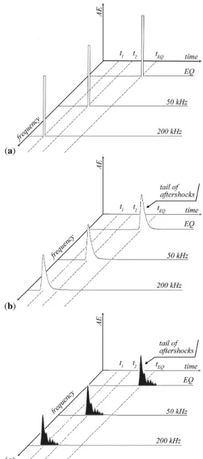
Fig. 1. (a) The bulk of the frequency of the released AE decreases
vs. time, and, as a first order approximation, the phenomenon can be depicted in terms of Dirac δ-functions. (b) Upon closer physical consideration, every δ-function ought to be substituted by a log-normal distribution. (c) An eventual externally applied additional effect (such as e.g. tidal modulation) sometimes results into an ap-parent trend looking like a damped oscillation. See text. Figure af-ter Paparo and Gregori (2003) and Gregori and Paparo (2004). EQ means earthquake. During the rising phase of the lognormal dis-tribution the physical system is in “hammer regime” (see Sect. 5), while during the tail it is in “recovery phase”.
and continuous bodies, and infinitesimal calculus does not hold in the quantum domain. Even the Maxwell’s laws are “thermodynamic” expressions of phenomena that ought to be more properly described by means of photons and
Feyn-man graphs. In the same way, the kinetic theory of gases is a more detailed description of the laws of thermodynamics. But the usual model based on a “fog of billiard balls” cannot give justice for phase transitions, even with the refinement of the van der Waal’s equation. Consider that PC and portable telephones had not be exploited by means of the Maxwell’s laws alone, and quantum mechanics and solid state physics were essential. Similarly, AE (ultrasounds) are often used by engineers for investigating the vibrations of structures, also referring to accelerometers, etc. But such approach in no way can be compared with the concern of the present paper, which is rather focused on the prime response of the atomic and molecular structures for diagnosing the very beginning of the ageing of materials, which testify a reduction of per-formance of the solid materials.
2 Preliminaries
2.1 The AE source
An AE source is associated with the release of energy origi-nated by the yield of some chemical bonds within some crys-tal structure. The reaction chain concept applies, because one additional chemical bond is more likely (eventually) to yield close to the point where the mechanical strength of the solid object is comparatively weaker, due to the presence of some previous flaw. It is the principle idea justifying the cleavage plane of a crystal fracture.
Differently stated, an AE signal can propagate through an ideal perfect elastic structure – i.e. through an ideal “solid” or “rigid” body. But it can release no AE, as the potential energy of every elastic bond is periodically transformed into kinetic energy – and viceversa. In contrast, the AE release oc-curs only whenever a bond yields and some energy becomes available for propagating a newly generated AE.
The opposite extreme – compared to an ideal “elastic” structure – refers to the case history of an ideal “Newtonian fluid”, where every displacement of some part of the system is always strictly proportional to the applied stress. This is the ideal “plastic” behaviour. Every such ideal body eventu-ally transports AE, although by causing a damping, depend-ing on the internal friction of the fluid.
Every physically existing body shall never be either an ideal solid or an ideal fluid. It is up to the researcher – who (according to Einstein and others) must seek “simple” or “beautiful” models for her/his interpretation – deciding whether the physical system of her/his concern can fit ei-ther one such simplifying extrapolation to the case history of an “ideal” body. In general, one finds that only one such model is suited, provided that suitable account is given for the implicit approximations that constrain the reliability of the model within some given physical boundaries.
2.2 The time sequence of the AE release
The first yielding bonds are associated with geometrical sizes typical of the most elementary crystal structure. Owing to the aforementioned reaction-chain mechanism, the newly yield-ing bonds produce a coalescence – of some former flaws of comparatively smaller size – into larger size flaws. Hence, the typical geometrical size of the flaws increases with time, and the frequency of the released AE consequently decreases. The principle is the same as the sound emitted by a violin cord when the geometrical length of the cord is progressively increased.
Therefore, the bulk of the frequency of the observed AE decreases vs. time (Fig. 1; Paparo and Gregori, 2003). As a first order approximation, the phenomenon can be de-picted in terms of Dirac functions, where every such δ-function is centred on some given AE frequency. However, upon closer physical consideration – i.e. upon considering that flaws of some given comparatively smaller size are still evolving while the population of some larger size flaws is already in progress – every such δ-function ought to be sub-stituted by a lognormal distribution. In addition, an even-tual externally applied additional effect (such as e.g. a tidal modulation) sometimes results into displaying some appar-ent trend looking like a damped oscillation. Such effect was observed e.g. either in volcanic AE records (Vesuvius), or in
AE records in a tectonically active area (the Raponi site). For
both such examples refer to Paparo and Gregori (2003). In the case of a seismic event, the AE are observed first at comparatively higher frequency, i.e. the HF AE. Then, pro-gressively lower frequency AE (i.e. LF AE) are observed. Then, the seismic roar is listened, and later on the me-chanical vibrations are detected by accelerometers, or by some specific mechanical structures within buildings, etc. Finally, whenever the AE frequency is decreased down to
∼0.5÷1 Hz, the destructive shock occurs.
The aforementioned oscillation of the tail of the lognor-mal distribution, which is characteristic of the AE events, is similar to – though physically different compared to – the well known time series of earthquakes that is called of “af-tershocks”. In fact, it has to be stressed that the aftershocks of an earthquake are caused by a different mechanism. Con-sider e.g. a bar that is subjected to an external mechanical action, until it breaks into two parts. Such parts are subjected to the same action, and are further broken, each one into two smaller bars, etc. Every such event generates a shock, re-sulting into a time series of events, which in general are of decreasing intensity, etc. This is the rationale for the genera-tion of earthquakes, which is much different compared to the aforementioned AE case history, where the mechanism rather appeals to the timing of the coalescence of flaws associated with the generation of AE of decreasing frequency. The final result is apparently the same, although the physical timing relies on a different physical justification.
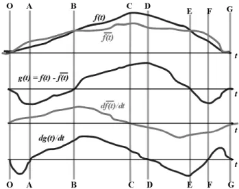
Fig. 2. Qualitative cartoon showing an arbitrary observational
da-tum f (t), with its smoothing average over a suitable time interval, and its residual, and their respective time derivatives. See text.
In general, therefore, it has to be expected that the HF
AE are representative of the comparatively earlier stages of
the evolution of the system. For instance, in the case of the crustal stress, the release of HF AE reflects the former exter-nally applied tectonic action. In contrast, the comparatively lower frequency AE, i.e. the LF AE, do reveal some processes or phenomena that occur within the physical system when its original ideal “solid” crystal structure already suffered by some relevant ageing, or deterioration. Therefore, in the case of crustal stress, it has to be expected that the LF AE records appear more correlated with tectonic agents, compared to the
HF AE that respond rather to some former trigger, occurring
when the crystal structure was still almost perfectly shaped. In such same respect, it ought to be pointed out that the infor-mation provided by accelerometers or by seismometers deals with a much evolved stage of the evolution of the system, and it applies when a “thermodynamic” description can be significantly applied in terms of continuous functions, dif-ferential calculus, and of vibrations of structures. However, such much later stage of the phenomenon cannot be repre-sentative of the original crustal stress propagation that was the real precursor of the processes that originally triggered the mechanism that finally led to the catastrophic yield.
As a general rule - while dealing with every specific actual application – both HF AE and LF AE ought to be monitored, and their respective inferences suitably analysed. In fact, on some occasions either one AE or the other results compara-tively more effective, depending on the kind of phenomenon that results more sensible concerning the final effect to be monitored or forecasted. In addition, consider that – on a few case histories here reported and dealing with some early investigations on AE – only one AE frequency was recorded.
726 G. Gregori et al.: Fatigue, ageing, and catastrophe of solid structures
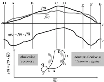
Fig. 3. Qualitative cartoon, showing how to infer the “hammer
regime” vs. the “recovery regime”
2.3 The AE probe
It should be pointed out that an AE recording device is com-posed of the sensor set with amplifier, etc. and data logger, plus in addition some whole part of the same physical system being monitored. In fact, if the AE sensor (i.e. the acoustic transducer) monitors e.g. some solid outcrop (granite, lime-stone, lava, etc.), it records the AE released within such en-tire (approximately) “solid” object up to some large distance from the transducer itself. Such distance cannot be envisaged a priori, as it depends on two crucial physical factors: the in-tensity of the prime AE source, and the damping of the signal, while it propagates from its source through the transducer.
In any case, the entire composite recording device, com-posed of the transducer plus the entire “solid” object – up to some suitable and unknown distance from the transducer – has to be considered as a unique probe. Such fact has impor-tant consequences. For instance, while monitoring a small lava outcrop (e.g. a dyke) on the flanks of Vesuvius, indeed we do monitor a large fraction of the entire volume of its vol-canic edifice, due to the (unknown) underground extension of the natural probe represented by some kind of elongated “tongue” of solidified lava.
Under such favourable circumstances, the large size of the probe – and its effectiveness in transporting AE – do imply an excellent signal-to-noise ratio in the final records. 2.4 The prime cause for the AE release
Distinction ought to be made between an “external” vs. an “internal” forcing as the prime cause that triggers the AE re-lease.
The “external” forcing can be either exogenous or endoge-nous. For instance, a tectonic stress resulting from a geo-dynamic action results into a stress applied to some solid
Fig. 4. Qualitative cartoon, showing the “hammer plot” for inferring
“hammer regime” vs. “recovery regime”.
portion of the crust, causing the yield of some of its crystal bonds: it is an exogenous trigger. In contrast, an endogenous action or trigger is typically associated e.g. with the diffu-sion, at some high pressure, of some hot fluid through the pores of the “solid” body. Such pressure stress originates crystal bond yielding and AE release. That is, even an en-dogenous trigger is a cause that operates “externally” with respect to the crustal structure of concern.
The “internal” forcing is rather concerned with the physio-logical evolution of the system, after having suffered by some external action. That is, the physical system – after having been subject to some “external” action – goes through some recovery state, and – while spending such transient state dur-ing which it seeks some new equilibrium configuration – it eventually releases AE. This is an “internal” trigger, as no external action is implied, either by some mechanical stress, or by some endogenous fluids or other: it is just a natural evolution of the system, after having suffered by some “ex-ternally” applied paroxysm.
2.5 AE transmission vs. teleconnection
Some relevant physical concern deals with the maximum dis-tance at which an AE release can be detected – and such concern was the likely prime cause of the limited amount of previous investigation carried out in the natural environ-ment by means of AE. In fact, as a standard, the AE damp off within some very short distance through loose material, resulting practically useless for any monitoring purpose.
Hence, whenever AE records are monitored at sites located at ∼ several 100 km from their likely source – and such cor-relation appears observationally unquestionable – such ob-servational fact can be explained either by AE transmission or by AE teleconnection.
AE transmission ought to require the existence of some
waveguide, such as some kind of “rigid”, “solid”, uninter-rupted structure connecting AE source and AE recording site. Such physical condition, however, is likely to occur in homo-geneous bodies, such as within a man-made machinery, or in concrete buildings or constructions, etc., while it is unlikely to occur in natural structures – except at most under very ex-ceptional circumstances.
AE teleconnection rather implies that a common cause
triggers the AE prime action (exogenous or endogenous), which is responsible for the AE release that is recorded at different sites. AE teleconnection typically occurs in natu-ral structures (crustal slabs, volcanic edifices, etc.). For in-stance, according to clear observational inference, the entire Italian peninsula can be likened to one unique “solid” crustal slab, which is eventually stressed by some externally applied geodynamic action, by which crises of release of AE are si-multaneously monitored at sites even ∼ several hundred km far apart from each other.
3 F ≡ Forcing
The intensity of the AE signal is larger for a comparatively more intense applied forcing, although in general such rela-tion is not linear. Several such examples were found.
A diurnal (mostly thermoelastic, and partly tidal) effect was clearly recognised on a massif in the central Apennines (Gran Sasso). During day-time warming, the outer layers of rocks (limestone and dolomite) expand over the innermost rock volume, which is cooler and more contracted. In con-trast, during night-time, the outer rock layers, while cooling, do contract outside the warmer and more expanded rocks. Hence, during night-time, i.e. during rock cooling, a greater amount of AE release is monitored. The difference of such daily variation – when comparing different days – results from the different solar heating of the mountain depending on meteorological conditions. Refer to Gregori and Paparo (2004).
At the Raponi site (located in Orchi, hamlet of Foligno town, in central Italy), and in the Kefallin`ıa island (west-ern Greece), an annual wave of crustal stress was clearly recognised. The present interpretation is in terms of a wave of crustal stress crossing the entire Greek and Italian areas, maybe of planetary scale and origin. Additional investiga-tions are needed in order to assess the diagnostic potential of such unexpected and clear evidence. Refer to Paparo et al. (2006) and Poscolieri et al. (2006, 2006a) for additional details and discussion.
The F information also resulted into a series of seemingly clear and significant earthquake precursors. Three such case histories ought to be recalled.
At the site Giuliano, close to Potenza (southern Italy), sev-eral geophysical monitoring devices were in operation dur-ing the days that preceded the earthquake that occurred on 3
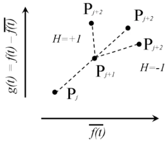
Fig. 5. Qualitative cartoon, showing a three-point detail of a
“ham-mer plot”. Consider three consecutive points Pj, Pj +1, Pj +2. Draw the line through Pj and Pj +1. If Pj +2falls to the left of such line it is concluded that Pj +2is associated with a state of H≡1, if to the right of the line H≡ −1. If Pj +2falls right on such line, Pj +2is associated with a state of H≡0.
Fig. 6. Qualitative cartoon, showing a general trend of a point
se-quence on a “hammer plot”. Suppose that the leading physical trend is suggestive of an counterclockwise behaviour (dashed line). Ob-servational errors, however, produce a scatter of the plotted points (solid line). According to the procedure sketched in Fig. 5, the re-sult shall appear like a series of both H =+1 and H =−1, with a prevailing component of H =+1 values. The concern is about en-visaging a significant filter aimed at focusing in some objective and unquestionable way the leading physical trend, independent of the perturbation produced by the scatter originated by the observational errors.
April 1996, of magnitude Md=4.6 with epicentre at ∼18 km from the AE recording site. Some ∼2 days before the shock, the LF AE intensity went out of scale for a time lag of
∼1 day. The existence of a teleconnection mechanisms over
∼18 km distance is an observational fact, although it is es-sentially unexplained.
On the Italian peninsula, the HF AE intensity – recorded at several 100 km from the epicentre – displays a violent crisis
728 G. Gregori et al.: Fatigue, ageing, and catastrophe of solid structures
Fig. 7. HF AE “hammer plot” for the Raponi site during 2004.
some ∼7÷8 months before the shock, and the LF AE some
∼2 months before the shock. Such inference was checked on a few occasions. Refer to Paparo et al. (2006) for details.
Concerning the Kefallin`ıa Island (western Greece) – in ad-dition to the aforementioned HF AE annual wave – a stress soliton was recorded (mainly in the LF AE), presumably crossing the entire area and lasting several months. The as-sessment and recognition of actual earthquake precursors, however, need for some much longer series of records. In any case, the much different tectonic setting – compared to the Italian peninsula – justifies an expectedly much differ-ent behaviour. Refer to Poscolieri et al. (2006) for details. Concerning AE records in volcanic areas, the volcano Pe-teroa (Argentina, in the Planchon volcanic complex) displays regular bursts of HF AE that envisage a clear tidal control. The volcanic edifice operates like the valve of a pressure cooker: whenever the ebb-and-flow of the tide lifts the weigh of the valve, a burst of endogenous hot fluids – which are no more constrained by the valve – produces a peak of AE re-lease (Ruzzante et al., 20071). That is, the volcano Peteroa appears to respond with a surprisingly great precision to the tidal trigger.
4 T ≡ Time or “ageing”
The focus is on the fatigue of the material. It is some kind of ultrasonic yelp, or whine, or moan, or whimper, which is independent of the intensity of the applied forcing, and it is only related to the ageing of the material. That is, the in-tensity F of the AE signal is related to the strength of the applied stress (Sect. 3). But the timing of the AE release
re-1Ruzzante, J., L`opez Pumarega, M. I., Piotrowski, R., Gregori,
G. P., Paparo, G., Poscolieri, M. and Zanini, A.: Acoustic emission (AE), tides and degassing on the Peteroa volcano (Argentina), in preparation, 2007.
Fig. 8. HF AE “hammer plot” for the Kefallin`ıa island during 2004.
flects the evolutionary stage of the reaction chain process (see Sect. 2.1). Such information is clearly inferred by applying a fractal analysis to the recorded AE signal.2
The Giuliano (Potenza) case history (Sect. 3) showed a progressive decrease – lasting for at least 2 months – from an LF AE fractal dimension Dt∼1 (equivalent to full non-organization of the fracture surface) to Dt ∼0.45÷0.4 (the null value for Dt corresponds to perfect organization of the fracture into a cleavage plane). The records were collected at Giuliano, i.e., at ∼18 km distance from the epicentre. But the same inference resulted to apply also for the Colfiorito earthquake, which had epicentre much farther away. How-ever, concerning the records at the Raponi site – i.e. collected right at the epicentre of the Colfiorito earthquake – the LF AE fractal dimension Dt, showed no equivalent clear evidence referring to the Molise earthquake. The earthquake precur-sor was very clear in the F effect (for both HF AE and LF
AE), though it was not evident in the LF AE fractal
dimen-sion Dt. The problem requires harder thinking on a wealthier database. See Paparo et al. (2006).
Concerning the Kefallin`ıa case history, both HF AE and
LF AE fractal dimensions Dtcould be evaluated during some exceedingly short time lag for getting any relevant useful in-ference – upon considering the particularly complicated tec-tonic setting of the area. See Poscolieri et al. (2006).
The AE records in volcanic areas (Vesuvius and Stromboli) resulted particularly effective.
2The original signal is first smoothed by a weighted running
average over 24 hours time interval, in order to get rid of all diurnal effects (thermoelastic and/or tidal). The residual – between original record and smoothed average – is investigated by selecting a series of relative maxima above some suitable threshold. The time series of such relative maxima – i.e. a so-called point-like process – is then analysed by fractal analysis.
In the Vesuvius case, the LF AE Dt resulted much effec-tive (Paparo et al., 2004). Whenever the endogenous pressure pushes the hot fluids into the pores of the solid parts of the volcanic edifice, the crystal bonds yield in some random way – deriving from a process of 3-D diffusion – and it is found
Dt ∼1. In contrast, when the endogenous pressure of the hot fluids has a temporary decrease, the volcanic edifice – being no more supported by the endogenous pressure – can temporarily experience several micro-collapses, and the re-leased AE displays Dt<1. In this way, it is possible to assess – using tout court an intuitive though expressive term – when Vesuvius is “inflating”, compared to the times when it is “de-flating”. The effect is clear in LF AE, while it is less clear for
HF AE (see Sect. 2.2).
It should be pointed out that such interpretation is further supported by the aforementioned evidence got about the vol-cano Peteroa (Sect. 3).
In addition, concerning seismic activity on Vesuvius – and consistently with the expectation of such interpretation – dur-ing “inflation” time a conspicuous seismic activity is ob-served, although resulting into a series of a large number of instrumental shocks. In contrast, during “deflation” time the activity is concentrated in a few shocks of larger intensity. The integral of the total energy release during “inflation” is much larger than the integral during “deflation”.
Concerning Stromboli, the HF AE Dt gave a much clear precursor – with an advance of at least 5 months – of the cri-sis that occurred at the end of 2002 (see Gregori and Paparo, 2006). It should be pointed out that the F of HF AE gives a completely different information compared to the fractal dimension Dt, thus confirming the (expected) fact that dif-ferent physical parameters give difdif-ferent inferences.
5 H =“Hammer” effect
Every phenomenon can be distinguished into two opposed physical states, i.e. whether it is subject to some forcing, or in contrast whether it is rather in a stage of recovery. Dif-ferently stated, such distinction depends one whether the AE release occurs due to an active external forcing, or rather due to its “aftershock” recovery. Let us briefly call such distinc-tion the “hammer effect”, envisaging that – during forcing – the system is like being hit by a hammer, while – during re-covery – it seeks a new equilibrium after the hammer stroke. “Hammer time” will be conventionally defined by an index
H ≡1, and “recovery time” by an index H ≡−1, while even
the indeterminate case history H ≡0 will be eventually con-sidered.
Such general principle – and the evaluation of H – can be operatively applied as follows. For clarity purposes, refer to the qualitative cartoon of Fig. 2.
Let some given (arbitrary) physical measurement being represented by a function f (t ). Call f (t )some moving aver-age over a suitable time lag (computed accordingly, and
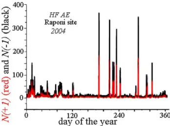
be-Fig. 9. Total number of H =+1 (red) and H =−1 (black) computed
per day for HF AE at the Raponi site during 2004.
ing either weighted or not). Call g(t )=f (t )−f (t ) the resid-ual. Then, suppose to plot df (t )/dt and dg(t )/dt vs. t.
Plot (Fig. 3) dg(t )/dt vs. df (t )/dt and – by a little think-ing – promptly realise that the “hammer regime” corresponds to a counterclockwise trend over such plot. In contrast, a “re-covery regime” corresponds to a clockwise rotation.
The same result is attained by plotting (Fig. 4)
g(t )=f (t )−f (t )vs. f (t ), which will be briefly called “ham-mer plot”.
If one applies such “hammer” analysis to an ideal lognor-mal trend – such as the one qualitatively represented in Fig. 1 – it is found that the smaller is the radius of the loop on the “hammer plot” the sharper is the lognormal distribution. Or the width of the lognormal distribution determines the size of the loop in the hammer diagram. Therefore, plotting the loop permits recognising, almost in real time, when a struc-ture is subject to slow or fast deformations (such as during fault slippage etc.).
Practical application of the “hammer plot” is carried out as follows. Consider three consecutive points Pj, Pj +1, Pj +2 plotted on the “hammer plot” (Fig. 5). Draw the line through Pj and Pj +1. If Pj +2falls to the left of such line state that Pj +2is associated with a state of H ≡1, if to the right of the line H ≡ −1. If Pj +2falls right on such line state that Pj +2 is associated with a state of H ≡0.
A crucial point is concerned with the role of errors. If the physical system is experiencing e.g. a “hammer state”, its “hammer plot” shall result counterclockwise (Fig. 6). The plotted points, however, are subject to the observational er-rors, which shall produce a scatter of the plotted points around the leading counterclockwise trends. Therefore, the sequence of computed H values shall contain some large number of H ≡ −1 randomly included into some compara-tively larger ensemble of H ≡1.
730 G. Gregori et al.: Fatigue, ageing, and catastrophe of solid structures
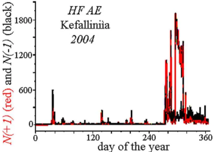
Fig. 10. Total number of H =+1 (red) and H =−1 (black)
com-puted per day for HF AE at the Kefallin`ıa Island during 2004.
The concept is better explained in terms of an intuitive – though, strictly speaking, not rigorous – analogy. Con-sider the trajectory of a molecule within the stream of a fluid, which shows a Brownian motion along its average flow line. The track of points drawn in the “hammer plot” shows some scatter equivalent to such Brownian motion, clustered around a main flow line, which is the information of physical con-cern for investigating the hammer effect. In the ultimate anal-ysis, natural phenomena occur independent of the way they are observed and described. The hammer effect analysis is just an expressive way of representing some parameter – de-rived by a suitable analysis of observations – that ought to help in focusing on some leading and large scale characteris-tics of the evolution of the physical system.
Therefore, every computed series of H values must be suitably treated statistically, in order to smooth out the dev-astating role of the scatter caused by the observational errors. Such algorithms shall be assessed after suitable harder think-ing, and several concrete checks-and-trial applications to dif-ferent case histories. Only very few such applications are here presented, while a systematic re-handling is currently in progress of all AE data series available to the authors.
Figure 7 shows the “hammer plot” of the HF AE moni-tored at the Raponi site during 2004. Apart some lesser os-cillations, there is some approximate seasonal trend from the left (February) through June (extreme right) returning half-way at the centre of the plot in December. But no interpre-tation seems as yet possible, being the likely consequence of a change in the “external” tectonic actions that are applied to the area.
Much different appears the HF AE “hammer plot” for 2004 in the Kefallin`ıa island (Fig. 8). The difference between Figs. 7 and 8 are certainly concerned with the respective tec-tonic settings of the two regions.
Such difference can be further inspected by counting the total number of H =+1(red) and H =−1(black), at the
Raponi site (Fig. 9) and at Kefallin`ıa (Fig. 10). At the Raponi site, hammer and recovery regimes appear correlated and varying synchronously. In contrast, at Kefallin`ıa the tectonic setting implies close and repeated “hammer” strokes, mainly during October ÷ November.
The physical interpretation of such different inferences shall require harder thinking, and simultaneous consideration of the F, H, T effects associated with both HF AE and LF
AE, including their apparent correlation with the seismic
ac-tivity within some suitably large area around the AE record-ing site (in progress).
No simple intuitive model seems as yet possible, and a full understanding of phenomena could require an array of simultaneous AE recording stations, collected during some long time lag.
Some harder thinking is needed. The F , H , T information got by HF AE and LF AE – recorded in the natural environ-ment – envisages intriguing possibilities that, however, have to be physically interpreted by a cross-reference with differ-ent tectonic settings, and with differdiffer-ent applied “external” geodynamic actions. Similar and/or analogous investigations are to be carried out in the laboratory, concerning all materi-als used in buildings or in machineries, in order to inspect the potential applications for security and/or for the recovery of ageing structures (e.g. Carpinteri et al., 2007). At present, it appears premature giving an account of such achievements. Acknowledgements. The authors express their gratitude to A. Raponi and A. M. Raponi for kindly hosting the AE monitoring apparatus in the basement of their house at Orchi (Italy) and to the Greek colleagues who have been collecting the AE data in the Kefallin`ıa island. In addition, we thank I. Marson for several enlightening discussions, and for financial support in managing the Kefallin`ıa island measurements.
Edited by: P. F. Biagi
Reviewed by: two anonymous referees
References
Carpinteri, A., G. Lacidogna, and G. Niccolini,: Acoustic emis-sion monitoring of medieval towers considered as sensitive earth-quake receptors, Nat. Hazards Earth Syst. Sci., 7, 251–261, 2007, http://www.nat-hazards-earth-syst-sci.net/7/251/2007/.
Cello, G. and Malamud, B. D. (Eds): Fractal analysis for natural hazards, Geol. Soc. Lond., Special Publ., 261, 1–172, 2006. Gregori, G. P. and Paparo, G.: The Stromboli crisis of 28÷30
December 2002, Acta Geod. Geophys. Hung., 41(2), 273–287, 2006.
Gregori, G. P. and Paparo, G.: Acoustic emission (AE). A diag-nostic tool for environmental sciences and for non destructive tests (with a potential application to gravitational antennas), in Schr¨oder, 166–204, 2004.
Paparo, G., Gregori, G. P., Taloni, A., and Coppa, U.: Acoustic emissions (AE) and the energy supply to Vesuvius – “Inflation” and “deflation” times, Acta Geod. Geophys. Hung., 40(4), 471– 480, 2004.
Paparo, G. and Gregori, G. P.: Multifrequency acoustic emissions (AE) for monitoring the time evolution of microprocesses within solids, Reviews of Quantitative Nondestructive Evaluation, 22, AIP Conference Proceedings, edited by: Thompson, D. O. and Chimenti, D. E., 1423–1430, 2003.
Paparo, G., Gregori, G. P., Poscolieri, M., Marson, I., Angelucci, F., and Glorioso, G.: Crustal stress crises and seismic activity in the Italian peninsula investigated by fractal analysis of acous-tic emission (AE), soil exhalation and seismic data, In Cello and Malamud, 47–61, 2006.
Poscolieri, M., Lagios, E. Gregori, G. P., Paparo, G., Sakkas, V. A., Parcharidis, I., Marson, I., Soukis, K., Vassilakis, E., An-gelucci, F., and Vassilopoulou, S.: Crustal stress and seismic ac-tivity in the Ionian archipelago as inferred by combined satellite and ground based observations on the Kefallin`ıa Island (Greece), In Cello and Malamud, 63–78, 2006.
Poscolieri, M., Gregori, G. P., Paparo, G., and Zanini, A.: Crustal deformation and AE monitoring: annual variation and stress-soliton propagation, Nat. Hazards Earth Syst. Sci., 6, 961–971, 2006a.
Schr¨oder, W. (Ed.): Meteorological and geophysical fluid dynam-ics (A book to commemorate the centenary of the birth of Hans Ertel), Arbeitkreis Geschichte der Geophysik und Kosmische Physik, Wilfried Schr¨oder/Science, Bremen, 417 pp., 2004.