HAL Id: hal-02565261
https://hal.sorbonne-universite.fr/hal-02565261
Submitted on 6 May 2020
HAL is a multi-disciplinary open access
archive for the deposit and dissemination of
sci-entific research documents, whether they are
pub-lished or not. The documents may come from
teaching and research institutions in France or
abroad, or from public or private research centers.
L’archive ouverte pluridisciplinaire HAL, est
destinée au dépôt et à la diffusion de documents
scientifiques de niveau recherche, publiés ou non,
émanant des établissements d’enseignement et de
recherche français ou étrangers, des laboratoires
publics ou privés.
Energy and helicity fluxes in line-tied eruptive
simulations
L. Linan, E. Pariat, G. Aulanier, K. Moraitis, G. Valori
To cite this version:
L. Linan, E. Pariat, G. Aulanier, K. Moraitis, G. Valori. Energy and helicity fluxes in line-tied eruptive
simulations. Astronomy and Astrophysics - A&A, EDP Sciences, 2020, 636, pp.A41.
�10.1051/0004-6361/202037548�. �hal-02565261�
https://doi.org/10.1051/0004-6361/202037548 c L. Linan et al. 2020
Astronomy
&
Astrophysics
Energy and helicity fluxes in line-tied eruptive simulations
L. Linan
1, É. Pariat
1, G. Aulanier
1, K. Moraitis
1, and G. Valori
21 LESIA, Observatoire de Paris, Université PSL, CNRS, Sorbonne Université, Université de Paris, 5 place Jules Janssen,
92195 Meudon, France
e-mail: luis.linan@obspm.fr
2 Mullard Space Science Laboratory, University College London, Holmbury St. Mary, Dorking, Surrey RH5 6NT, UK
Received 22 January 2020/ Accepted 26 February 2020
ABSTRACT
Context.Conservation properties of magnetic helicity and energy in the quasi-ideal and low-β solar corona make these two quantities relevant for the study of solar active regions and eruptions.
Aims.Based on a decomposition of the magnetic field into potential and nonpotential components, magnetic energy and relative helic-ity can both also be decomposed into two quantities: potential and free energies, and volume-threading and current-carrying helicities. In this study, we perform a coupled analysis of their behaviors in a set of parametric 3D magnetohydrodynamic (MHD) simulations of solar-like eruptions.
Methods.We present the general formulations for the time-varying components of energy and helicity in resistive MHD. We cal-culated them numerically with a specific gauge, and compared their behaviors in the numerical simulations, which differ from one another by their imposed boundary-driving motions. Thus, we investigated the impact of different active regions surface flows on the development of the energy and helicity-related quantities.
Results.Despite general similarities in their overall behaviors, helicities and energies display different evolutions that cannot be
explained in a unique framework. While the energy fluxes are similar in all simulations, the physical mechanisms that govern the evolution of the helicities are markedly distinct from one simulation to another: the evolution of volume-threading helicity can be governed by boundary fluxes or helicity transfer, depending on the simulation.
Conclusions.The eruption takes place for the same value of the ratio of the current-carrying helicity to the total helicity in all sim-ulations. However, our study highlights that this threshold can be reached in different ways, with different helicity-related processes dominating for different photospheric flows. This means that the details of the pre-eruptive dynamics do not influence the eruption-onset helicity-related threshold. Nevertheless, the helicity-flux dynamics may be more or less efficient in changing the time required to reach the onset of the eruption.
Key words. magnetic fields – Sun: photosphere – Sun: corona – Sun: flares – magnetohydrodynamics (MHD) – Sun: activity
1. Introduction
Magnetic helicity is a volume-integrated ideal magnetohydro-dynamic (MHD) invariant describing the level of twist and entanglement of the magnetic field lines. Initially introduced by Elsasser (1956), magnetic helicity is a conserved quantity within the ideal MHD paradigm (Woltjer 1958). However, the strict definition of Elsasser is gauge invariant only for magnet-ically bounded system, a condition that is not satisfied in most cases, such as the solar atmosphere. This led to the introduction byBerger & Field (1984) andFinn & Antonsen(1985) of the relative magnetic helicity, a gauge-invariant quantity suitable for use in solar physics and more generally for natural plasmas.
Using a numerical simulation,Pariat et al.(2015) confirmed the hypothesis introduced by Taylor (1974) that even in pres-ence of nonideal processes, the dissipation of magnetic helicity is negligible. Relative magnetic helicity cannot be dissipated or created within the corona, therefore it can only be transported or annihilated. This conservation property has several major con-sequences, one of which might be that coronal mass ejections (CMEs) are the consequence of the evacuation of an excess of helicity (Rust 1994;Low 1996).
In recent years, magnetic helicity has been at the heart of many studies dealing with various topics such as the generation
of solar eruptions (e.g., Kusano et al. 2004; Longcope & Beveridge 2007; Priest et al. 2016), magnetic reconnection (e.g.,Linton et al. 2001;Linton & Antiochos 2002;Del Sordo et al. 2010), solar filaments (e.g., Antiochos 2013; Knizhnik et al. 2015;Zhao et al. 2015), and solar and stellar dynamos (e.g.,
Brandenburg & Subramanian 2005;Simon 2012).
Magnetic energy is another relevant quantity in MHD with which eruptivity in the solar corona is studied because most of solar events are driven magnetically (e.g.,Schrijver & Zwaan 2008). From the point of view of the energetic budget, magnetic energy is the only source of energy that can generate the pow-erful events that are observed in the solar atmosphere, such as coronal mass ejections, flares, and solar jets (Forbes 2000). Mag-netic energy can be decomposed into a current-carrying energy, known as free energy, and a potential energy (cf. Sect. 3.1). Solar flares and CMEs are characterized by a rapid change of the coronal magnetic field that does not change the radial com-ponent of the photospheric field. Because the potential field is determined by the radial magnetic field at the photosphere, only the free energy can therefore be converted into kinetic and ther-mal energies during fast coronal events (Aulanier et al. 2009;
Karpen et al. 2012). The potential energy thus represents the lowest energy state of the magnetic field in the solar corona (e.g.,
Priest 2014).
Open Access article,published by EDP Sciences, under the terms of the Creative Commons Attribution License (https://creativecommons.org/licenses/by/4.0),
An analysis of magnetic energies combined with a study of magnetic helicities appears a powerful tool for characterizing active regions and their evolutions toward eruptive events. How-ever, measuring these quantities from observational data remains challenging. One possibility is to estimate the accumulation of magnetic helicity and energy in the solar corona by integrating their fluxes across the solar photosphere over time (Kusano et al. 2002;Nindos et al. 2003;Yamamoto et al. 2005;Yamamoto & Sakurai 2009). This method cannot trace the coronal evolution and requires high-cadence time-series magnetograms as well as the velocity fields on the photosphere. Because no direct obser-vation of the photospheric velocity is available, it is obtained by inferring the magnetic field on the solar surface. Despite the progress made in deducing the velocity field (Kusano et al. 2002;
Welsch et al. 2004;Longcope 2004) as well as further improve-ment on flux estimations (Pariat et al. 2005; Chae 2007; Liu & Schuck 2012,2013;Dalmasse et al. 2014,2018), the com-putation of magnetic energy and helicity fluxes remains very sensitive to the method that is used and to the quality of the observations. A different approach is to compute energy and helicity in coronal volumes. Because magnetic energy and helic-ity are volume integrals, properly computing them with this method requires the full 3D knowledge of the magnetic field in the volume that is studied. Currently, only 2D measurement on the solar surface are provided, therefore a 3D extrapolation of the magnetic field is a necessary step. The diverse methods based on the volume-integration approach for estimating the magnetic relative helicity were benchmarked inValori et al.(2016). Di ffer-ent solar active regions have previously been investigated (Valori et al. 2013;Moraitis et al. 2014,2019; Guo et al. 2017;Polito et al. 2017;Temmer et al. 2017;James et al. 2018;Thalmann et al. 2019).
In parallel, the properties of both helicity and energy are still being studied in solar-like parametric simulations.Berger(2003) introduced the decomposition of the relative magnetic helicity into two gauge-invariant components: a current-carrying helic-ity related to the current-carrying magnetic field, and a comple-mentary volume-threading helicity.Pariat et al.(2017) followed and estimated these quantities in a set of seven simulations of the formation of solar active regions (Leake et al. 2013,2014). The different simulations led to either stable or eruptive config-urations. The authors found that it is possible to distinguish the two configurations by studying the ratio of the current-carrying helicity to the relative helicity. The ratio before the eruption indeed presents high values only in the eruptive case. To bet-ter understand the properties of the relative helicity decomposi-tion,Linan et al.(2018) provided the first analytical formulae of the time-variation of nonpotential and volume-threading helic-ity. They also computed and followed them in two simulations ofLeake et al.(2013,2014) and in a simulation of the generation of a coronal jet (Pariat et al. 2005). They found that the current-carrying helicity does indeed not evolve as a result of boundary fluxes, but builds up through its exchange with the volume-threading helicity. The evolutions of the current-carrying and the volume-threading helicities are partially controlled by a transfer term that reflects the exchange between these two types of helic-ity. This exchange term dominates the dynamics of the current-carrying helicity at different instants of the simulations. This means that this helicity does not only evolve as a result of bound-ary fluxes. The eruption phases of these simulation follow the same dynamics: the current-carrying helicity is first transformed into the volume-threading helicity, and then the latter is ejected from the domain by boundary fluxes. Moreover, the transfer term is expressed as a volume integral: consequently, these two
helicities are not classically conserved quantities in the sense that they cannot be independently expressed as a flux through the boundaries, even in ideal MHD, unlike the relative magnetic helicity. This finding strengthens the knowledge of the proper-ties of nonpotential and volume-threading helicity that was first studied byMoraitis et al.(2014).
Zuccarello et al. (2015) presented 3D parametric resistive MHD simulations of solar coronal eruptions. Simulations are distinguished by the different motions (line-tied) applied on the photosphere with similar but distinct flux cancelation drivers. Their eruptions were driven by the torus instability (Aulanier et al. 2009;Démoulin & Aulanier 2010) and occurred at a pre-cise time identified by a series a relaxation runs. Recently, these models were used to investigate the increase in the downward component of the Lorentz force density around an polarity-inversion line in comparison with the photospheric observation (Barczynski et al. 2019). From these simulation,Zuccarello et al.
(2018) studied the impact of the different boundary driving flows on the helicity and energy injection. They found that the helic-ity ratio of the current-carrying helichelic-ity to the relative helichelic-ity is clearly associated with the eruption trigger because the erup-tions within the different runs took place exactly when the ratio reached the very same threshold value.
Recently, the first preliminary observational tests confirmed the idea that the helicity ratio is a good predictor of eruptiv-ity. Based on 3D extrapolation and using different nonlinear force-free models, the time evolution of the helicity ratio has been investigated in three active regions: AR 12673 inMoraitis et al.(2019), the most active of the cycle 24; and AR 11158 and AR 12192 in Thalmann et al. (2019), two extensively studied active regions that generated eruptive and confined flares. How-ever, complementary studies are still needed to understand how the different magnetic topologies observed in the solar corona are linked to the dynamics of the helicity ratio.
In the present study, we apply the helicity decomposition to the analysis of the simulations ofZuccarello et al.(2015,2018) to investigate the time-variations of the different types of mag-netic energy and helicity. In particular, we are interested in the way that the different boundary motion influence the helicity and energy dynamics.Zuccarello et al.(2018) showed that the dif-ferent boundary motions lead to different efficiency in injecting helicity and energy in the domain. In the present work, we aim to explain the physical processes that are responsible for these differences: are they related to boundary fluxes, dissipation, or volume evolution? We also examine whether the transfer term between the two helicity components plays a major role in the helicity budgets, as has been observed inLinan et al.(2018).
Additionally, we study the dynamics of the helicities in comparison with the dynamics of their energy counterparts, for instance, current-carrying helicity and free energy, and volume-threading helicity and potential energy. Our goal is to highlight the differences and the similarities in the helicity and energy buildup. This study aims to improve our knowledge on mag-netic helicities and energies, and it is a necessary step to better understand the full topological and energetic complexity of solar active regions.
Our paper is divided into different sections that are orga-nized as follows. First, we present the time-variation of nonpo-tential and volume-threading helicities (see Sect.2). In the same way, we then introduce the different components of the magnetic energy and also their time-variation written for the specific case of resistive MHD (see Sect.3). After presenting the simulations (see Sect.4), we present the time evolution of the different quan-tities (see Sect.5). Using our set of simulations, we investigate
the role of the transfer term between the helicity components in their evolutions (see Sect.6). While we investigate the di ffer-ence in helicity dynamics in Sect. 7, we focus on the similari-ties between magnetic energy and helicity fluxes in Sect.8. In the conclusion, we discuss the effect of the different boundary-driving motions on the energy and helicity injection and on the eruptivity helicity ratio.
2. Nonpotential and volume-threading helicities
In the fixed volume V bounded by the surface S , the magnetic helicity is defined as
Hm= Z
v
A · B dV, (1)
with A the vector potential of the studied magnetic field B, i.e ∇ ×A= B. In practice, this scalar description of the geometrical properties of magnetic field lines is general only if the magnetic field is tangential to the surface, that is, if V is a magnetically bounded volume. The magnetic helicity is gauge invariant if and only if this condition is respected. For the study of natu-ral plasmas, especially in solar physics, the magnetic field does not satisfy this condition, the solar photosphere being subject to significant flux. Berger & Field(1984) introduced the relative magnetic helicity, a gauge-invariant quantity, based on a refer-ence field. Throughout the paper, we use the potential referrefer-ence field Bp that has the same normal distribution of B throughout the surface S and satisfies
(
∇ ×Bp= 0
n · (B − Bp)|S = 0, (2)
where n is the outward-pointing unit vector normal on S . The potential field can thus be defined by a scalar function, such as ∇φ = Bp, and φ is the solution of the Laplace equation,
( ∆φ = 0 ∂φ
∂n|S = (n · B)|S.
(3) When Ap is the vector potential of the potential field Bp= ∇ × Ap, the relative magnetic helicity provided by
Finn & Antonsen(1985) is defined as Hv =
Z
v
( A+ Ap) · (B − Bp) dV. (4)
In this form, the relative magnetic helicity is independently invariant to gauge transformation of both A and Ap. The dif-ference between the potential field and the magnetic field can be written as a nonpotential magnetic field, Bj= B− Bp, associated with the vector Aj, defined as Aj= A − Ap, such as ∇ × Aj= Bj. When we use this unique decomposition of B and following the work ofBerger(2003), Eq. (4) can be divided into two gauge-invariant quantities: Hv = Hj+ Hp j (5) Hj= Z v Aj·BjdV (6) Hp j= 2 Z v Ap·BjdV, (7)
where Hj is the current-carrying magnetic helicity associated with only the current-carrying component of the magnetic field Bj, and Hp j is the volume-threading helicity involving both B
and Bp. By construction, both Hj and Hp j are gauge invariant because by virtue of Eq. (3), Bjhas a vanishing normal compo-nent on the surface.
In resistive MHD, where E= −u × B + η∇ × B (η being the resistivity, which is here assumed to be constant),Linan et al.
(2018) established the following equation for the time evolution of the current-carrying magnetic helicity Hj:
dHj dt = dHj dt Diss + dHj dt Bp, var + dHj dt Transf + FVn, Aj+ FBn, Aj+ FAj, Aj+ Fφ, Aj+ FNon-ideal, Aj (8) with dHj dt Diss = −2Z v η(∇ × B) · BjdV (9) dHj dt Transf = −2Z v (u × B) · BpdV (10) dHj dt Bp, var = 2Z v ∂φ ∂t∇ ·AjdV (11) FVn, Aj= −2 Z S (B · Aj)u · dS (12) FBn, Aj = 2 Z S (u · Aj)B · dS (13) FAj, Aj= Z S Aj× ∂ ∂tAj· dS (14) Fφ, Aj= −2 Z S ∂φ ∂tAj· dS (15) FNon-ideal, Aj= −2 Z S η(∇ × B) × Aj· dS . (16)
From this decomposition,Linan et al.(2018) obtained an equa-tion for the time-variaequa-tion that is composed only of gauge-invariant terms: dHj dt = dHj dt Own + dHj dt Diss + dHj dt Transf , (17) with dHj dt Own = dHj dt Bp, var + FNon-ideal, Aj + Fφ, Aj+ FVn, Aj+ FBn, Aj+ FAj, Aj. (18) All these terms initially provided by Linan et al. (2018) are recalled here because we analyze them and comment on them in the next sections.
Similarly, the time evolution of the volume-threading mag-netic helicity Hp jcan be decomposed as
dHp j dt = dHp j dt Diss + dHp j dt Bp, var + dHp j dt Transf + FNon-ideal, Ap + FVn, Ap+ FBn, Ap+ FAj, Ap+ Fφ, Ap (19)
with dHp j dt Diss = −2Z v η(∇ × B) · BpdV (20) dHp j dt Transf = 2Z v (u × B) · BpdV (21) dHp j dt Bp, var = 2Z v ∂φ ∂t∇ · ( Ap−Aj) dV (22) FVn, Ap = −2 Z S (B · Ap)u · dS (23) FBn, Ap= 2 Z S (u · Ap)B · dS (24) FAj, Ap= 2 Z S Aj× ∂ ∂tAp· dS (25) Fφ, Ap= −2 Z S ∂φ ∂t( Ap−Aj) · dS (26) FNon-ideal, Ap= −2 Z S η(∇ × B) × Ap· dS . (27)
The time-variation of Hp jcan also be constructed with gauge-invariant terms only:
dHp j dt = dHp j dt Own + dHp j dt Diss − dHj dt Transf (28) with dHp j dt Own = dHp j dt Bp, var + FNon-ideal, Ap + FVn, Ap+ FBn, Ap+ FAj, Ap+ Fφ, Ap. (29) These decompositions were obtained without any particular hypothesis on the gauge that is used. In particular, we are free to use the Coulomb gauge for A and Ap. With this choice, the volume terms dHj/dt Bp, varand dHp j/dt
Bp, varboth vanish. Thus dHj/dt Own and dHp j/dt
Ownonly contain boundary-flux contri-butions. The transfer term dHj/dt
Transf expresses the exchange between the helicities Hj and Hp j without any consequence on the evolution of the total relative helicity HV. Furthermore, this quantity being a volume term, the time-variations of Hjand Hp j cannot be expressed solely through boundary fluxes. Therefore Hj and Hp j are not conserved quantities in resistive or ideal MHD.
3. Magnetic energy
3.1. Free and potential energies
With the decomposition of the magnetic field into current-carrying and potential components, B= Bp+ Bj, the total mag-netic energy Evcan be also decomposed as
Ev= 1 8π Z v B2dV = Ep+ Ej+ 1 4π Z S φBj· dS − 1 4π Z v φ∇ · BjdV, (30) with Ep= 1 8π Z v B2 pdV Ej= 1 8π Z v B2 jdV. (31)
In this decomposition, Ej is the energy of the current-carrying magnetic field, also known as free energy, and Ep the energy of the solenoidal magnetic field. Because the potential field shares the same surface distribution as the total magnetic field, the surface integral vanishes in Eq. (30). Numerically, the dis-cretization of the mesh grid unavoidably induces a finite level of non-solenoidality (∇ · B , 0), and consequently, the last term in Eq. (30) is not exactly null (cf.Valori et al. 2013). However, considering a solenoidal field, Eq. (30) can be simplified into
Ev= Ej+ Ep. (32)
This decomposition is similar to the decomposition of the helic-ity obtained in Eq. (5). However, here, the potential energy Ep, unlike the volume-threading helicity, only depends on the poten-tial field without a dependence on the nonpotenpoten-tial field. 3.2. Time-variation of the total magnetic energy
We aim to determine the time-variation of the total magnetic energy Evin a fixed volume V,
dEv dt = 1 4π Z v B ·∂B ∂t dV. (33)
In the resistive MHD, we use the Faraday law, ∂B/∂t= −∇ × E, and we obtain 1 4π Z v B ·∂B ∂t dV= − 1 4π Z v B · ∇ × E dV = 1 4π Z v B · ∇ × (u × B) dV (34) − 1 4π Z v B · (∇ × (η∇ × B)) dV.
Using the Gauss divergence theorem, we can decompose the first term of Eq. (34): 1 4π Z v B · ∇ × (u × B) dV= 1 4π Z S (u × B) × B · dS (35) + 1 4π Z v (u × B) · (∇ × B) dV. Here, the surface term corresponds to the surface integral of the poynting vector and can be divided into two terms:
1 4π Z S (u × B) × B · dS = − 1 4π Z S (B · B)u · dS + 1 4π Z S (u · B)B · dS . (36)
Finally, assuming for simplicity that the resistivity is constant in space, the variation of the total magnetic energy can be decom-posed as dEv dt = dEv dt Diss+ dEv dt var+ FBn, E+ FVn, E , (37) with dEv dt Diss= − 1 4πη Z v B · (∇ × (∇ × B)) dV (38) dEv dt var= 1 4π Z v (u × B) · (∇ × B) dV (39) FBn, E = 1 4π Z S (u · B)B · dS (40) FVn, E = − 1 4π Z S (B · B)u · dS . (41)
We performed a similar time variation for Ev as Linan et al. (2018) did for helicities as we summarized in Sect.2. We find two fluxes: FVn, E a shearing term associated with horizontal motion, and an emerging term FBn, E that is related to the emer-gence. Longcope et al. (2007) decomposed the shearing term at the photospheric level into two contributions by di fferentiat-ing the motion between the different flux patches and the spin motion of isolated flux patches. As with Hjand Hp j, the time-variation of Ev cannot be expressed through boundary fluxes, and thus Ev is not a conserved quantity. Even in ideal MHD, when dEv/dt|Diss is null, a volume term dEv/dt|var survives. Unlike dHj/dt and dHp j/dt, the time-variation of the total energy Evdepends on neither A nor Ap: each term of Eq. (37) is gauge invariant.
3.3. Time-variation of the potential and free magnetic energies
Similarly to the analysis of dEv/dt in the previous section, it is possible to obtain the time-variation of Ep. Using the scalar potential φ of Bp such as ∇φ = Bp and the Gauss divergence theorem, we write dEp dt = 1 4π Z v Bp· ∂Bp ∂t dV = 1 4π Z v Bp· ∂∇φ ∂t dV = Fφ,Bz+ dEp dt |ns, (42) with Fφ,Bz = 1 4π Z S ∂φ ∂tBp· dS (43) dEp dt |ns= − 1 4π Z v ∂φ ∂t(∇ · Bp) dV. (44)
For a purely solenoidal potential field, dEp/dt|nsis null and thus the time-variation of Ep is written in a simple way as a single surface term depending on the variation of the potential field. A decrease in potential energy can therefore be associated in par-ticular with a cancelation at the polarity-inversion line (PIL) or a dispersion of the potential magnetic field. Unlike Ev, Epis a conserved quantity in resistive MHD.
For the study of the evolution of nonpotential energy Ej, the easiest way is to consider only the difference between the decom-positions obtained from Eqs. (37) and (42):
dEj dt = dE dt − dEp dt · (45)
Still, this identity is truly accurate only in the case of purely solenoidal magnetic fields, that is, ∇ · Bj= 0 and when Bj|S = 0 (cf. Sect.3.1). Hereafter, we therefore introduce a generic for-mulation where terms that explicitly account for nonsolenoidal errors are retained,
dEj dt = 1 4π Z v Bj· ∂Bj ∂t dV (46) =dEv dt + dEp dt − 1 4π Z v B ·∂Bp ∂t dV − 1 4π Z v Bp· ∂B ∂t dV. The last two terms on the right are very similar to dEp/dt and dEv/dt. They can thus be decomposed in the same way,
−1 4π Z v B ·∂Bp ∂t dV= − 1 4π Z S ∂φ ∂tB · dS+ 1 4π Z v ∂φ ∂t(∇ · B) dV, (47) and −1 4π Z v Bp· ∂B ∂t dV= 1 4πη Z v Bp· (∇ × (∇ × B)) dV − 1 4π Z v (u × B) · (∇ × Bp) dV − 1 4π Z S (u · Bp)B · dS + 1 4π Z S (B · Bp)u · dS .
By definition, the curl of the potential field is null, and thus the second volume integral on the right-hand side formally vanishes. Finally, by grouping all the terms, the time-variation of the non-potential magnetic energy can be written as
dEj dt = dEj dt Diss + dEj dt var + FBn, Ej+ FVn, Ej (48) + dEj dt ns + Fφ, Bj, with dEj dt Diss = − 1 4πη Z v Bj· (∇ × (∇ × B)) dV (49) dEj dt var = 1 4π Z v (u × B) · (∇ × B) dV (50) FBn, Ej= 1 4π Z S (u · Bj)B · dS (51) FVn, Ej= − 1 4π Z S (B · Bj)u · dS (52) Fφ, Bj= − 1 4π Z S ∂φ ∂tBj· dS (53) dEj dt ns = 1 4π Z v ∂φ ∂t(∇ · Bj) dV. (54)
As expected, the decomposition we obtain is similar to the one obtained with dEv/dt (see Eq. (37)). The dissipation term dEj/dt|nsis null if the magnetic field is solenoidal. However, we compute it in order to quantify the effect of purely numerical errors.
4. Line-tied eruptive simulations
In order to comparatively analyze the evolution of helicities and energies and to study the time-variation of the energy, we used magnetic field data produced by parametric 3D MHD simula-tions of eruptive events of the solar corona that were initially presented inZuccarello et al.(2015).
For this set of simulations, the OHM-MPI code (Aulanier et al. 2005) solves MHD equations in the system’s nondimen-sional units for a volume covering the domain x ∈ [−10, 10], y ∈ [−10, 10] and z ∈ [0, 30]. The employed mesh is nonuni-form and the smallest cell is centered at x= y = z = 0. In order to facilitate the computation of the energies and helicities, our study was performed on a subdomain excluding the z= 0 plane, interpolated into a uniform Cartesian grid composed of 333 cells in the x and y direction, and 500 cells in the z directions. The resulting analyzed volume is x ∈ [−10, 10], y ∈ [−10, 10] and z ∈ [0.006, 30]. As a result of the interpolation on a uniform
Fig. 1.Applied boundary-driving motions for the four different numerical experiments. White represents the positive polarity (Bz(z= 0.006) > 0)
and black the negative polarity (Bz(z= 0.006) < 0). Orange and cyan arrows indicate the distribution of the velocity flows we applied to the
negative and positive polarity, respectively.
grid (whose cell sizes are 0.06, to be compared to the original grid, whose cell sizes range from 0.006 to 0.32), the magnetic field we obtained has a lower solenoidality than the initial grid. This reduces the accuracy of the magnetic helicity and energy computations (Valori et al. 2016).
The system is delimited by a set of boundaries subject to “open” boundary conditions (except at z = 0). In the ana-lyzed datasets, the bottom boundary is at z = 0.006, one mesh point above the surface corresponding to the photospheric level where line-tied boundary conditions were imposed in the orig-inal numerical experiments. All the physical MHD quantities, such as the magnetic field, can leave the simulation domain through lateral and top boundaries during the evolution of the system.
Four parametric simulations were performed, all starting with a common phase that is referred to as the “shearing phase” inZuccarello et al.(2015,2018). Initially, the magnetic field is potential and generated by two unbalanced and asymmetric sub-photospheric polarities. During the shearing phase, asymmetric vortices centered around the local maxima of |Bz(z= 0)| slowly evolve the initial potential magnetic field into a current-carrying magnetic field. This shearing flow motion induces a magnetic shear close to the PIL and at the end of this phase, creates a current-carrying magnetic field arcade surrounded by a quasi-potential background field. During this entire phase, the distri-bution of Bz at the bottom boundary remains unchanged. This phase lasts from the time t= 10tAuntil t= 100tAin the system time coordinate, where tAis the reference Alfvén time used in
Zuccarello et al.(2015).
Then the four parametric simulations differ by the motion pattern that is imposed at the bottom boundary (cf. Fig.1). We refer to this phase as the “pre-eruption” phase. In a first motion profile, labeled “convergence” (Fig. 1, left panel), the veloc-ity flows only follow the horizontal direction x and are only applied close to the PIL. This creates a cancellation of the mag-netic flux around the PIL but only slightly affects the periph-ery of the active regions. Unlike the previous case, for the run labeled “stretching” (Fig.1, middle left panel), these horizontal motions are also applied at the periphery of the active region. For the other two runs, labeled “dispersion central” and “dispersion peripheral” (Fig.1, middle right and right panels), the motions spread in all directions from the center. The only difference is in the portion of the active region that is subjected to these motions. In the dispersion peripheral run, only the periphery of the active region is concerned, while in dispersion central, the dispersion also occurs in the center of the polarity where the magnetic field is strongest.
The four runs all present a cancellation of magnetic flux at the PIL that is permitted by a finite photospheric diffusion. The sheared-arcade configuration at the end of the shearing phase evolves into a bald-patch topology, and the magnetic reconnec-tion process leads to the formareconnec-tion of a flux rope. The system then evolves until it reaches the instant where it becomes unsta-ble and erupts (cf.Aulanier et al. 2009, for a description of the eruption process). The onset of the eruption, that is, the time t1 of the onset of the instability, is accurately determined by a series of relaxation runs for each simulation (Zuccarello et al. 2015). It occurs at t1= 196, 214, 220 and 164tAfor the conver-gence, stretching, dispersion peripheral, and dispersion central runs, respectively.
To ensure the numerical stability of the code, a finite resis-tivity η and a pseudo-viscosity ν are necessary (Zuccarello et al. 2015). During the common shearing phase until t < 100tAand during the pre-eruption phase, the coronal diffusivity is ηcor = 4, 8 × 10⁻⁴ and the pseudo-viscosity is fixed to ν0 = 25. After the eruption, during a phase referred to as eruption phase, ηcor is 2, 1 × 10⁻³ and ν0 is 41, 7. To allow later flux cancellation at the PIL, a photospheric resistivity ηphot = ηcor = 4, 8 × 10⁻⁴ is imposed only during the pre-eruption phase. The photospheric resistivity is set to zero in the shearing phase and before the erup-tion. The change in resistivity follows a ramp-down time profile during the time t1− 5tA < t < t1+ 5tA. This transitional period is called “eruption onset phase” and is represented as the yellow band in all the figures. We note that the time t1 corresponds to the middle of the ramp-down time profile, therefore the bound-ary flows are null only at t > t1+ 5tA. In this paper, we removed the first mesh point in the z-direction, which corresponds to the bottom boundary level. We therefore have a uniform resistivity throughout the domain in order to facilitate the calculation of the so-called “nonideal” terms.
5. Energy and helicity evolutions
In this section we first introduce the method for numerically computing the energies and helicities in our set of simulations. Then, we discuss the computation of the time-variations. 5.1. Energy and helicity estimations
In order to compute the different helicities and energies at each time tA, we used the method of Valori et al.(2012). The dat-acubes of the magnetic field B, of the plasma-velocity field u, and of the plasma thermodynamic quantities allowed us to com-pute all the quantities that appear in Eqs. (8), (19), (48), and (42).
Fig. 2.Evolution of the different magnetic helicities (top panels), from left to right: relative magnetic helicity (Hv, Eq.(4)), volume-threading
helicity (Hp j, Eq.(7)), and current-carrying helicity (Hj, Eq.(6)). Time evolution of the different magnetic energies (bottom panel), from left to
right: total magnetic energy (Ev, Eq.(32)), potential energy (Ep, Eq.(31)), and free energy (Ej, Eq.(31)). The different simulations are dispersion
central (red line), dispersion peripheral (green line), stretching (yellow line) and convergence (blue line). The yellow vertical band corresponds to the onset phase of the eruption.
First the scalar potential φ(t) of the potential magnetic field Bp(t) was obtained from a numerical solution of the Laplace Eq. (3). The numerical methods we employed to solve this equa-tion required an uniform grid and thus led to the interpolaequa-tion of the initial grid, as mentioned in Sect.4. The potential vectors A(t) and Ap(t) were computed according to Eq. (14) inValori
et al.(2012) and follow the DeVore-Coulomb gauge defined in
Pariat et al.(2015):
∇ ·Ap= 0 (55)
Az(x, y, z, t)= Ap,z(x, y, z, t)= 0. (56)
This choice of gauge was complemented by the following rela-tionship inherent in the integration method:
A(x, y, z= ztop, t)⊥= Ap(x, y, z= ztop, t)⊥, (57) where ⊥ means the normal component. It corresponds to the 1D integration of magnetic fields starting at the top boundary of the domain at height ztop. Finally, we obtained the helicities and energies from Eqs. (5) and (30). In Fig.2we plot the time evolution of these quantities for the different runs. In order to facilitate the comparison between the different runs, the time is plotted with a modified time variable t − t1in each figure, where t1 is the onset time defined in Sect. (4) and is different for each of the four simulations.
Unlike Zuccarello et al. (2018), we are interested here in the evolution of the quantities after the common shearing phase, including the eruption phase (which was not studied by
Zuccarello et al. 2018). We also recall that the domain studied here is slightly different from the one studied inZuccarello et al.
(2018) (cf. Sect.4). Figure2shows that the dynamics of energies and helicities are qualitatively similar from one simulation to the
other during the three different phases. The different boundary-forcing mainly affects the magnitude of the different quantities, but not the quality of their dynamical behaviors.
We also note that the dynamic of helicities and energies changes during the eruption. For the current-carrying helicity, Hj, and the free energy, Ej, we observe an overall increase dur-ing the pre-eruption phase, followed by a decrease durdur-ing the eruption phase. The quantities related to the potential magnetic fields, Ep and Hp j, both decrease in the pre-eruption phase. In the eruption phase Epremains constant while Hp jcontinues to decrease, although at a lower rate than in the pre-eruption phase. Because both Hj and Hp jdecrease, the relative helicity Hv also decreases in the eruption phase. The total energy, Ev, has a dynamics similar to Hv: the system loses energy throughout the simulation, but at a different rate before and after the eruption.
Overall, the behavior of the helicities is similar to their energy counterparts, for example, Hvto Ev, Hjto Ej, Hp jto Ep. This is particularly visible for the current-carrying helicity and the free energy: when Hjincreases (decreases), Ejalso increases (decreases). In the next sections we focus more on the reasons of these trends by studying the fluxes of the different quantities. 5.2. Time-variation estimation
After all the vectors were calculated, we computed the instan-taneous time-variations of energies and helicities obtained from Eqs. (8), (19), (48), and (42). The surface integrals were calcu-lated systematically as the sum of the contributions from the six boundaries. A study focusing on the contribution of the lower boundary alone is conducted in Sect.9.3.
Linan et al. (2018) validated the time-variations equations established for the volume-threading helicity, Hp j, and the current-carrying helicity, Hj. The accuracy of the computation
Fig. 3.Left panel: time evolution of the instantaneous time-variation, dEv/dt (dashed black curves, Eq.(37)), and of the sum, dEj/dt + dEp/dt
(continuous blue curves, Eqs. (8) and (19)) for the dispersion peripheral run. Right panel: time evolution of the instantaneous time-variation, dHv/dt (dashed black curves, Eq. (23) inPariat et al. 2015, and of the sum, dHj/dt + dHp j/dt (continuous blue curves, Eqs. (8) and (19)) for the
dispersion peripheral run. The yellow bands correspond to the eruption onset phase.
is related to difference factors such as the discretization and the remapping of the data, spatial and temporal, as well as to nonex-plicit numerical diffusive terms that are not accounted for in our analytical resistive MHD model. In our study, we present a com-plementary test by comparing the time-variation of the relative helicity, dHv/dt computed from Eq. (23) inPariat et al.(2015), with the sum of the time-variations of nonpotential and volume-threading helicities, dHj/dt + dHp j/dt from (8) to (19). In this way, both sides are computed with the same temporal accuracy.
The result of this comparison is presented in the right panel of Fig.3. In this figure we plot dHv/dt and dHj/dt + dHp j/dt for the dispersion peripheral simulation. For the other runs, the dif-ference is on the same order of magnitude and varies in a similar way. We therefore do not plot this here. The difference is very low, with an average deviation smaller than 0.1%. This confirms the robustness of our calculation method as well as the validity of our analytical equations.
In the same way, we compare in Fig.3(left panel) the time-variation of the total magnetic energy, dEv/dt, computed from Eq. (37), with the sum of the time-variations of free and poten-tial energies, dEj/dt + dEp/dt, from Eqs. (42) to (48). Here, the difference is not negligible, with an average relative difference of 27%. The cause of this difference is likely mainly the non-solenoidality of the magnetic field. As mentioned Sect.3, with a finite level of non-solenoidality, the equality of Eq. (45) is not fully accurate because Ev, Ej,s+ Ep(see Sect.3.1).
In order to estimate the artificial non-solenoidal energy con-tributions,Valori et al.(2013) introduced the following decom-position:
Ev= Ej,s+ Ep,s+ Ep,ns+ Ej,ns+ Emix, (58) where Ej,sand Ep,s are the energies of the current-carrying and potential solenoidal magnetic field. Ej,ns and Ep,ns are the non-solenoidal components, whereas Emix corresponds to all the remaining cross terms. For a solenoidal field we have Ej,ns = Ep,ns = Emix = 0, Ej,ns = Ej, Ep,ns = Ep, and therefore dEj/dt + dEp/dt = dEv/dt.
The finite non-solenoidality (∇ · B , 0) affects the pre-cision of the helicity and energy computations, as studied by
Valori et al. (2016). Following Valori et al. (2013, 2016),
Thalmann et al. (2019), we used the energy criteria Ediv/Ev to quantify the non-solenoidality effect. The divergence-based energy is defined as
Ediv= Ep,ns+ Ej,ns+ |Emix|. (59)
For the four simulation analyzed in this paper we find an aver-age of Ediv/Ev ' 2%. According toValori et al. (2016), this value for the average of non-solenoidality leads to a precision of ≤6% for our helicity computations, which is much lower than the 27% discrepancy found in Fig. 3. One possible cause of non-solenoidality is our interpolation of the original data from a highly nonuniform mesh onto a uniform grid, which can increase the nondivergence of the magnetic field. Different tests have been made to degrade and also improve the interpolation to give a rough estimate of the effect. Finer interpolations, however, have required considering only a fraction of the whole numer-ical domain to keep the number of grid points manageable. The outcome of these tests is that neither presented results that dif-fered significantly from our baseline interpolation. In particu-lar, Ediv/Evalways remained on the order of 2%, which means that this error therefore seems intrinsic to the numerical mod-els. The level of interpolation chosen in our study therefore is a good compromise between the required computed power and the quality of our data. In addition, it is worth noting that vari-ous terms in our equations depend on time variations, so that the accuracy of our flux computations can also be limited by a rela-tive coarseness of the time outputs of the available data. Testing for this would require recalculating the simulations with a higher cadence for its outputs, which is beyond the scope of this paper.
6. Helicity transfer
As mentioned in the introduction (see Sect. 1), Linan et al.
(2018) showed for two different eruptive simulations that the exchange between Hp j and Hj is controlled by the gauge-invariant transfer term dHj/dt|Transf (see Eq. (10)), which there-fore plays a key role in evolving these helicities. In order to confirm these different results in the particular case of our line-tied simulations, we plot in Fig.4the gauge-invariant terms of dHj/dt (see Eq. (17)), and dHp j/dt (see Eq. (28)) for the conver-gence and the dispersion peripheral runs.
In the convergence case (see Fig.4, top left panel), the con-version of helicity from Hp j to Hj and the boundary flux have similar amplitudes during the pre-eruption phase. Both contribu-tions are positive, thus Hjincreases (e.g., dHj/dt is positive). The transfer term, dHj/dt|Transf, dominates the evolution of Hjwhen it is close in time to the eruption. Meanwhile, Hp j decreases mainly because of the strong helicity transfer (cf. Fig.4, top right panel), that is, dHj/dt|Transfis the dominating term of dHp j/dt. In
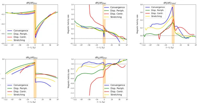
Fig. 4.Time evolution of the helicity variation rates, dHj/dt and dHp j/dt (dashed black curves; Eqs. (8) and (19)), of the helicity transfer term,
dHj/dt|Transfand dHp j/dt|Transf(solid red curves; Eqs. (10) and (21)), of the own terms, dHj/dt|Ownand dHp j/dt|Own(solid blue curves; Eqs. (18)
and (29)), and of the dissipation terms, dHj/dt|Diss and dHp j/dt|Diss(solid green curves; Eqs. (9) and (20)) for the convergence simulation (top
panels) and for the dispersion peripheral simulation (bottom panels). Left and right panels: evolution of the current carrying helicity, Hj, and
volume-threading helicity Hp j, respectively.
comparison, the flux of Hp jrelated to the own term, dHp j/dt|Own, is very low. This means that the injection of Hp jis not enough to compensate for its conversion to Hj.
Moreover, as with the flux emergence simulations presented inLinan et al. (2018), the eruption is accompanied by a sharp decrease of the transfer term. However, unlike in Linan et al.
(2018), the sign of dHj/dt|Transf does not change here during the onset phase of the eruption. During the eruption phase, the dissipation terms, dHj/dt|Dissand dHp j/dt|Diss, dominate the variation of the helicities. This is related to the increase in resistivity η imposed in the numerical experiment during that period.
In the dispersion peripheral simulation (see Fig. 4, bot-tom panels), the variations of Hj and Hp j during the pre-eruption phase are noticeably dominated by the boundary fluxes, dHj/dt|Ownand dHp j/dt|Own. The transfer terms are significantly less intense than the injection of Hj and Hp j, except close to the eruption. During the eruption phase, the dynamics is mostly dominated by the resistive dissipation terms, dHj/dt|Diss and dHp j/dt|Diss.
We thus observe that while the trends of Hj and Hp j are similar for the convergence and the dispersion peripheral sim-ulations, as discussed in Sect. 5, these variations are in fact due to noticeably different dynamics of the helicity fluxes. For instance, the decrease of Hp jin the pre-eruption phase is due to an intense conversion of helicity (high values of dHp j/dt|Transf)
for the dispersion peripheral simulation, whereas in the conver-gence run, a similar evolution of Hp jis explained by an intense negative boundary flux, dHp j/dt|Ownduring that period.
Finally, as has been noted inLinan et al.(2018), for both the simulations analyzed here but also for the two others, the transfer terms cannot be neglected. We confirm that the estimations of boundary fluxes are not sufficient to follow the dynamics of Hj and Hp j. However, unlike with the flux emergence and solar jet simulations studied inLinan et al.(2018), the precise mechanism of the buildup of Hj and Hp j does depend on the simulations during the pre-eruption phase. Studying this dependence is the goal of the next section.
7. Distinguishing between simulations in terms of helicity dynamics
In the previous section, we described that the magnitude of the different gauge-invariant helicity variation terms could be sig-nificantly different in the dispersion peripheral and in the con-vergence simulations. This demonstrates that even if the general trends of Hp jand Hjare similar (see Sect.5), their dynamics can be significantly different.
In order to estimate the effect of the different boundary driver, Fig.5 displays the different gauge-invariant variation terms for the four different numerical simulations: the boundary fluxes
Fig. 5.Time evolution of the different gauge invariant terms of dHj/dt (top panels), from left to right: dissipation term (dHj/dt|Diss, Eq.(9)), own
term (dHj/dt|Own, Eq.(18)), and helicity transfer term (dHj/dt|Transf, Eq.(10)). Time evolution of the different gauge invariant terms of dHp j/dt
(bottom panels), from left to right: dissipation term (dHp j/dt|Diss, Eq.(20)), and own term (dHp j/dt|Own, Eq.(29)). Each curve color corresponds
to a particular simulation: dispersion central (red line), dispersion peripheral (green line), stretching (yellow line), and convergence (blue line). The yellow band corresponds to the onset phase of the eruption.
dHj/dt|Ownand dHp j/dt|Own; the transfer term, dHj/dt|Transf; and the dissipations terms dHj/dt|Dissand dHp j/dt|Diss.
The dissipations terms (cf. Fig.5, left panels) are not signif-icantly different from one simulation to the other. The sudden increase in absolute values of the dissipations terms, observed during the eruption onset phase, is related to the imposed numerical increase in resistivity. The variations in magnitude, particularly in the pre-eruption phase, are minor compared to the variations in other gauge-invariant terms.
The boundary flux term dHj/dt|Ownis also very similar from one simulation to another, except for the dispersion central run, for which more nonpotential helicity is markedly injected dur-ing the pre-eruption phase (see Fig.5, middle top panel). Unlike dHj/dt|Own, the boundary flux of Hp j, dHp j/dt|Own, is strongly sensitive to the boundary-driving pattern (see Fig. 5, bottom left panel). Tthe sign and magnitude of dHp j/dt|Own depend on the simulation. For the dispersion simulations, there is a sig-nificant injection of negative Hp j, whereas in the convergence and stretching case, the flux is significantly weaker, if not of the opposite sign.
Finally, Fig.5(top right panel) shows that the helicity trans-fer rate, dHj/dt|Transf, is higher for the convergence and stretch-ing simulations than for the dispersion cases in the pre-eruption phase. Unlike with the other cases where the transfer term is almost constant during an early period, in the dispersion central run dHj/dt|Transfincreases from the first moments of the simula-tion.
In summary, we observed that during the pre-eruption phase, the increase of Hjand reciprocally the decrease of Hp j(cf. Fig.5) are not explained by the same physical process in the different simulations. We observe three significantly different dynamics:
– The convergence and stretching simulations present a similar dynamics for their fluxes of helicity. They are characterized
by a relatively weak boundary flux of Hp j counterbalanced by a strong transfer from Hp jto Hj. The own term of Hj is positive, involving an injection of current-carrying helicity. Its magnitude is almost identical in these two runs.
– For the dispersion peripheral run, Hp j decreases mostly because of the boundary flux, unlike with the previous cases. In comparison to the boundary flux, the transfer from Hp jto Hjis less important. The flux of Hjis similar to the conver-gence and stretching runs.
– The dispersion central shares some similarities with the dis-persion peripheral run regarding the variations of Hp j. How-ever, this simulation is characterized by a high boundary flux of Hjthat is distinct and significantly higher than the three other cases.
Finally, simulations with the largest injection of helicities due to their own terms (whether Hjor Hp j) have the lowest magnitude of the transfer term. Inversely, a strong exchange between Hjand Hp jis accompanied by lower fluxes through the surfaces. Both lead to a similar trend for the relative helicity Hv. This shows that the boundary fluxes of Hjor Hp jas well as the volume term, dHj/dt|Transf, are directly related to the morphology and the evo-lution of the magnetic field at the bottom boundary. In Sect.9.3
we discuss that a specific boundary-driven pattern may influence the different physical mechanisms of the evolution of the mag-netic helicities.
8. Distinguishing between simulations in terms of energy dynamics
As shown in Sect.5, the evolutions of Hjand Ejare very similar. Likewise, Hp j and Ep j evolve in the same way during the pre-eruption phase. The main difference appears after the eruption, where Hp jstill decreases while Ep jremains constant. However,
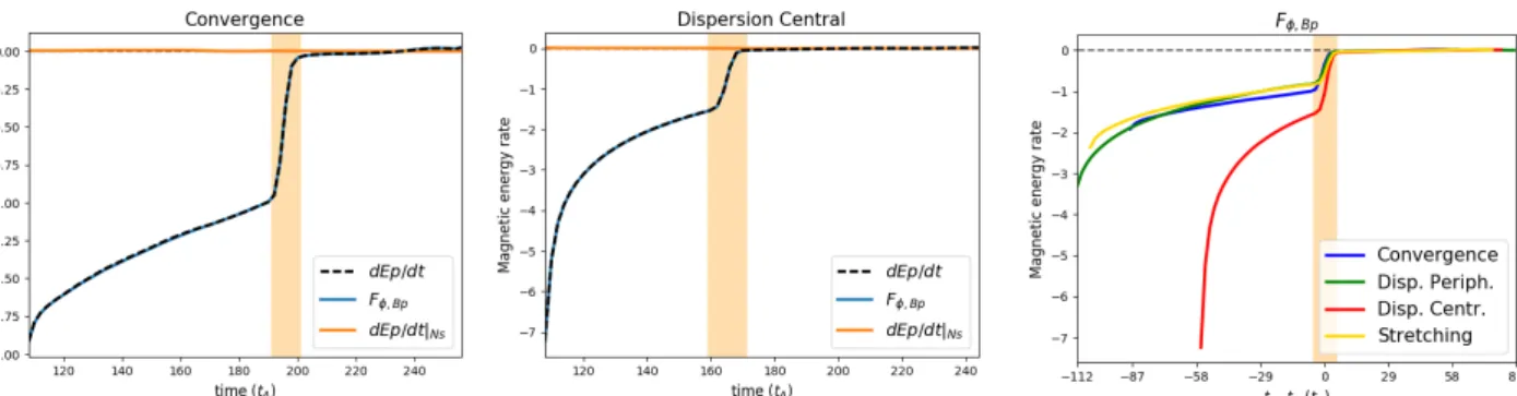
Fig. 6.Left and middle panel: time evolution of the potential energy variation term (dashed black line; dEp/dt; Eq. (42)) and the different terms
constituting the instantaneous time-variation of Ep(Eq.(42)): Fφ,Bz (blue line; Eq.(43)), and dEp/dt|ns(orange line; Eq.(44)). Left and middle
panels: evolution for the convergence and dispersion central simulation, respectively. Right panel: time evolution of Fφ,Bzfor the four simulations
dispersion central (red line), dispersion peripheral (green line), stretching (yellow line), and convergence (blue line). The yellow band corresponds to the onset phase of the eruption.
the similar overall behaviors of Hp j and Hj hide very different physical mechanisms, depending on the simulation, as shown in the previous section. We identified three types of evolution for the dynamics of the helicities. In this section we focus on the fol-lowing questions: how do Ep jand Ejevolve? Does the dynamics of the energy fluxes also distinguish between the different simu-lations, as the helicity dynamics do?
For this purpose, we present in Fig.6all the flux that appear in the decomposition of dEp/dt (see Eq. (42)) for the conver-gence (Fig.6, left panel) and the dispersion central simulations (Fig.6, middle panel). In both simulations, the nonideal term is almost null because of a very low non-solenoidality of the poten-tial field, for instance, ∇ · Bp' 0. The evolution of the potential energy therefore depends only on Fφ,Bz, which results from the
evolution of the magnetic field at the boundaries. During the pre-eruption phase, the magnitude of Fφ,Bzas the relative change of
the magnetic field at the boundary becomes weaker. Then, during the eruption onset phase, Fφ,Bzdecreases strongly before
becom-ing null durbecom-ing the eruption phase. The magnetic field is indeed kept fixed at the bottom boundary during that period.
From comparing Fφ,Bz in the different simulations, we note
that Fφ,Bzpresents the same evolution for all simulations except
for the dispersion central (see Fig.6, right panel). This indicates that except for the dispersion central simulation, the differences in boundary-driven motions do not affect the injection of the potential energy (cf. the discussion in Sect.9.3). However, this run has the same functional form as the other, is only more e ffi-cient, and therefore quicker, in achieving the eruption.
Regarding Ep, only the dispersion central run presents a dif-ferent behavior. The same conclusion was obtained for the fluxes of Hj, for instance, dHj/dt|Own (see Fig. 5, middle top panel), but not for dHp j/dt|Own (cf. Fig.5l). First, Fφ,Bz is negative for
the entire simulation, while the sign dHp j/dt|Owndepends on the simulation. This confirms that there is no direct link between the dynamics of Epand the injection of Hp j.
In Fig.7we observe the different terms of dEj/dt (Eq. (48)) for the four simulations. Unlike dHj/dt and dHp j/dt, the trends and dominant terms of dEj/dt are similar in the simulations. Only the magnitude of each term may differ. Before the eruption, dEj/dt is dominated by the emergence term FBn,Ej despite a
sig-nificant magnitude of the dissipation term, dEj/dt|Diss. Then, dur-ing the eruption, FBn,Ej becomes null as a result of the
interrup-tion of the boundary-driving flows. During the erupinterrup-tion phase, dEj/dt is negative and dominated by dEj/dt|Diss. The free energy mainly decreases because it is dissipated and not ejected out of the volume.
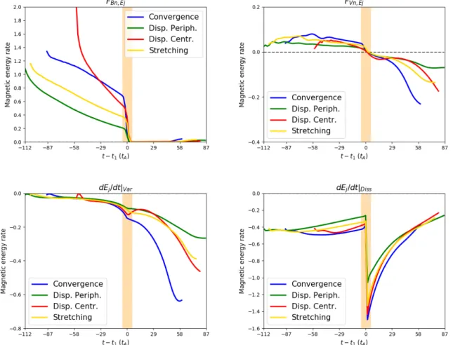
The dissipation term, dEj/dt|Dissdoes not vary much between the simulations (see Fig.8, bottom right panel). Similarly, the differences of FVn,Ej and dEj/dt|Varare small between the runs
during the pre-eruption phase. Only FBn,Ej (see Fig.7, top left
panel) presents significant differences in the simulations that affect the evolution of the free energy, Ej. The dispersion central simulation presents a distinctive trend. The magnitude of FBn,Ej
starts very high and then decreases to values similar to the other runs during the onset phase of the eruption.
Unlike the evolution of the helicities, Hj and Hp j, only the dispersion central simulation stands out from the other runs. This simulation is characterized by a higher decrease of the potential field (see Fig.6, right panel) and by a higher initial injection of Ejcaused by FBn,Ej(see Fig.8, top left panel). Before the
erup-tion, another difference with the helicities is that the variations of the trend of Ejand Epare purely related to the boundary fluxes. Finally, one key outcome of our study is that the dynamics of the energy fluxes do not distinguish between the simulations, unlike the helicity fluxes.
This shows that even if volume helicities and energies follow similar trends (cf. Fig.2), the physical mechanisms that drive their dynamics are very different. First, the evolution of free energy, Ej, and potential energy, Ep, are independent, while the current-carrying helicity, Hj, evolves in a correlated way with the volume-threading helicity, Hp j. Additionally, different bound-ary forcing only affects the magnitude of the energy fluxes. The dynamics of the helicity is more complex and varies drastically from one simulation to another. One group of simulations (dis-persion central and peripheral) is dominated by the flux through the surfaces, while a second group (convergence and stretching) is controlled by volume exchange within the domain. We con-clude that energy, helicity, and their decompositions have dis-tinct properties whose analysis should be complementary for the study of the eruptivity of active regions.
9. Discussion
9.1. Summary
In Sect.2we introduced the formulation of the magnetic rela-tive helicity, Hv, as well as the formulation of its decomposition into the current-carrying helicity, Hj, and the volume-threading helicity, Hp j. We also recalled the analytical equations of their time-variations obtained in Linan et al. (2018). Similarly, we introduced the decomposition of magnetic energy, Ev, into the sum of the potential energy, Ep, and the free energy, Ej. Then,
Fig. 7.Time evolution of the free-energy variation rate (dashed black line; dEj/dt; Eq. (48)) and the different terms constituting the instantaneous
time-variation of Ej(Eq.(48)): dEj/dt|Diss(blue line; Eq.(49)), dEj/dt|Var(orange line; Eq.(50)), FBn,Ej(green line; Eq.(51)), FVn,Ej(red line;
Eq.(52)), and dEj/dt|ns(purple line; Eq.(54)). Each panel corresponds to a different simulation: convergence (top left), stretching (top right),
dispersion peripheral (bottom left), and dispersion central (bottom right). The yellow band corresponds to the onset phase of the eruption.
we obtained the time-variation of Ev (see Eq. (37)), Ep (see Eq. (42)), and Ej(see Eq. (48)) by analytically deriving their time derivative (see Sect.3). These formulae are valid for any gauge choices and in the presence of finite level of non-solenoidality for the magnetic field.
Our numerical study of time-variations of energies and helicities is based on a series of four eruptive numerical MHD simulations of solar active regions (see Sect.4) that have been investigated inZuccarello et al.(2015). The evolution of each sim-ulation is characterized by different boundary forcing (line-tied) until the eruption (see Sect. 4). After the same shearing phase, four driving photospheric flows were considered: convergence, stretching, and peripheral and central dispersion flows. In this study we were particularly interested in the fluxes of energies and helicities during the flux rope formation, during the eruption onset phase, when the torus instability occurs, and during a short time interval after the eruption onset, called the eruption phase.
Initially, the magnetic energy, Ev, decreases as a result of the decrease in the potential magnetic field, Ep, despite the increase in free energy, Ej. At the same time, the decrease in volume-threading helicity, Hp j, compensates for the injection of the current-carrying helicity, Hj, which leads to a quasi-constant evolution of the relative helicity Hv (see Sect.5). The relative helicity was mostly injected during the earlier shearing phase.
The fluxes of free and potential energies, Ej and Ep (see Sect. 8) showed that the effectiveness of the buildup of free energy within the domain is purely related to the magnitude of one surface term. Similarly, the evolution of potential energy is fully linked with its boundary fluxes.
We also used these simulations to investigate the importance of the exchange between Hj and Hp j, which was previously highlighted by Linan et al. (2018). The exchange of helicity
between Hj and Hp j is controlled by a gauge-invariant term, dHj/dt|Transf(cf. Eq. (10)). As inLinan et al.(2018), we observed that this term plays a key role in the dynamics of both Hjand Hp j, in particular during the buildup phases where the transfer terms, dHp j/dt|Transf, dominate the evolution of dHp j/dt for the runs convergence and stretching. In the dispersion simulations, the evolutions of dHj/dt and dHp j/dt are dominated by their bound-ary fluxes, dHp j/dt|Ownand dHp j/dt|Own(cf. Eqs. (18) and (29)), even though the magnitude of the transfer term remains signif-icant. This means that neither Hj nor Hp j evolve as a result of boundary fluxes alone. This conclusion is consistent with the results of Linan et al. (2018) that were obtained for different numerical experiments. Specifically, Hjand Hp jcannot be esti-mated in observed active solar active regions by time integra-tion of its flux through the solar photosphere, but rather with a volume-integration method (Valori et al. 2016). This approach requires a 3D reconstruction of the coronal magnetic field from the 2D photospheric measurement with coronal field extrapola-tion techniques (Wiegelmann & Sakurai 2012;Wiegelmann et al. 2014). A more detailed discussion of the effect of the transfer term on the estimation of Hjand Hp jcan be found in the conclu-sion ofLinan et al.(2018).
The key outcome of the study is the observation that the dynamics of the transfer and fluxes of Hjand Hp jdepend on the simulation and thus on the imposed driving motions, even though the variations in Hjand Hp jseemed relatively independent of the simulation setup (see Sect.6). Despite the four boundary forcings, the different simulations remain very similar in terms of the mag-netic field topology. Nonetheless, the dominant terms of dHj/dt and dHj/dt are not the same from one simulation to another.
We highlighted three distinct types of dynamics of the evo-lution of the helicities in the simulations. In the convergence and
Fig. 8.Time evolution of the different gauge-invariant terms of dEj/dt: FBn,Ej(top right panel, Eq.(51)), FVn,Ej(top left panel, Eq.(52)), dEj/dt|Var
(bottom left panel, Eq.(50)), and dEj/dt|Diss(bottom right panel, Eq.(49)). The different colors present one simulation: dispersion central (red
line), dispersion peripheral (green line), stretching (yellow line), and convergence (blue line). The yellow band corresponds to the onset phase of the eruption.
stretching simulations, Hp jdoes not evolve as a result of bound-ary fluxes, but because of its conversion into Hj. The opposite is observed during the two dispersion simulations, for which the evolution of Hp jis mainly related to its fluxes through the bound-ary, with a weak transfer term. The dispersion central simula-tion stands out from the others because its boundary flux of the current-carrying helicity, Hj, is significantly higher.
Thus we were able to process several photospheric forcings to approach the diversity of active regions that are observed at the solar photosphere. We have come to the conclusion that the evo-lution of helicity during the formation of a flux rope is a complex process whose origin can be related to fluxes through the surface as well as to volume contributions.
9.2. Buildup of the helicity ratio
Zuccarello et al.(2018) have shown that the trigger of the erup-tions is related to a threshold in the helicity ratio Hj/Hv: this ratio reaches the same value, |Hj/Hv|thresh, for all simulations at the onset of the eruptions. In our runs, this threshold is 0.29 ± 0.01. However, as discussed in Sect. 7 ofZuccarello et al.(2018), the exact value of this threshold needs to be taken with care because relative helicity is not simply an additive quantity. We investi-gated how this helicity ratio is built up and eventually reached by studying the specific dynamics of Hjand Hp j(see Sects.6and7). Despite the different boundary forcings, the simulations are very similar, so that it might have been thought that the fluxes of Hj
and Hp jwould also be similar. However, the key outcome of our study is that the terms that dominate the evolution of dHj/dt or dHp j/dt sensitively depend on the simulation even if the overall trends are the same (Hjincreases and Hp jdecreases, see Sect.5). Three very distinct ways to reach the helicity eruptivity threshold were found. We observed that the eruption was trig-gered at a specific value of Hj/Hvindependently of the dynam-ics of Hjand Hp jto reach this threshold. Our work suggests that active regions could reach an eruptive state, either through strong increases of helicity fluxes or through magnetic configurations that induce strong helicity transfer.
The different ways to reach the helicity eruptivity threshold are not all equally effective. The eruption occurs more or less quickly after the end of the shearing phase. The dispersion cen-tral run is the most rapid simulation. Then we find the stretching and convergence runs, and last the dispersion peripheral case. The dispersion central simulation stands out from the others because it presents higher helicity fluxes (due to dHj/dt|Ownand dHp j/dt|Own) and energy fluxes (due to Fφ,Bzand FBn,Ej) than the
other cases.
Finally, using a set of resistive MHD simulations, we pro-vided new knowledge of the energy and helicity properties. In particular, our analytical and numerical work emphasizes recent studies (Pariat et al. 2017;Zuccarello et al. 2018;Moraitis et al. 2019;Thalmann et al. 2019) that demonstrated how promising the helicity ratio is as a marker of eruptivity. Further studies are still needed, whether to analytically establish the link between
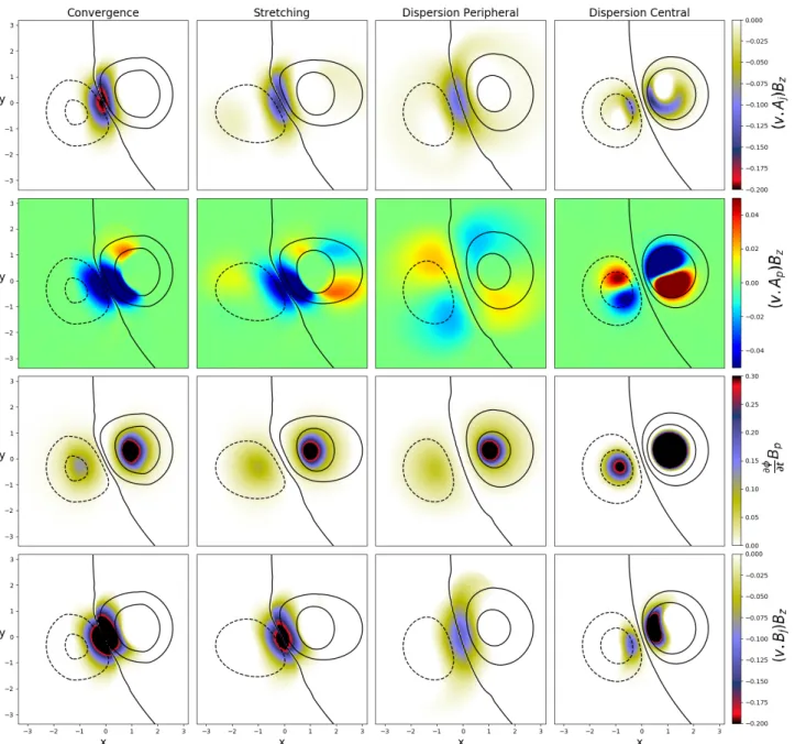
Fig. 9.From top to bottom: dimensionless magnitude of (v · Aj)Bz, (v · Ap)Bz, (∂φ/∂t)(Bp), and (v · Bj)Bzviewed in the (x, y) plane at z= 0.006,
at the relative time of t − t1 = −58. Isocontours of |Bz| (dashed line for negative values, solid line for positive values) correspond to values
of |Bz|= −4.5, −2.0, 0, 2.0, and 4.5. Each column in the panels presents one simulation, from left to right: convergence, stretching, dispersion
peripheral, and dispersion central.
the helicity ratio and torus instability or to properly estimate it from data that are measured in the solar atmosphere.
From direct observational data, the evolution of the ratio Hj/Hv was also analyzed in three active regions with different eruptive profiles. Moraitis et al. (2019) investigated the most active region of cycle 24 (AR 12673), while Thalmann et al.
(2019) focused on an eruptive and a confined flare (AR 11158 and AR 12192). These recent observational analyses seem to qualitatively confirm that the Hj/Hvratio is tightly related to the eruptivity of solar active regions.
9.3. Effect of the different flows on the helicity and energy injections
A key result of our study is that the specific driving flows that are applied at the bottom boundary are of significant importance on the dynamics of magnetic helicities and energies. They
influ-ence the magnitude and the sign of the own terms for the helicity as well as those of the main fluxes of dEj/dt and dEp/dt. More-over, as mentioned in the previous section, even if the way to reach the helicity eruptivity threshold matters less than reach-ing the threshold, the spatial velocity and magnetic distribu-tions at the boundary affect the time that is required to reach the threshold.
To reach an understanding of the effect of the line-tied forc-ing, we here briefly discuss the distribution of different quanti-ties at the bottom boundary. A more complete study is beyond the scope of the present paper but will be performed, however.
Our goal is to present quantities that might eventually be obtained from observed photospheric magnetograms. Figure9
shows four quantities that are related to the energy and helicity fluxes in a (x − y) view at z = 0.006 for all simulations at the same modified time to the eruption (t1− tA = −58): (v · Aj)Bz, the integrand of FVn,Aj, for the injection of Hj(see the first row