Step-by-step evaluation of photovoltaic module performance related to outdoor parameters: evaluation of the uncertainty

HAL Id: hal-01630076

https://hal.archives-ouvertes.fr/hal-01630076

Submitted on 26 Nov 2019

HAL is a multi-disciplinary open access

archive for the deposit and dissemination of

sci-entific research documents, whether they are

pub-lished or not. The documents may come from

teaching and research institutions in France or

abroad, or from public or private research centers.

L’archive ouverte pluridisciplinaire HAL, est

destinée au dépôt et à la diffusion de documents

scientifiques de niveau recherche, publiés ou non,

émanant des établissements d’enseignement et de

recherche français ou étrangers, des laboratoires

publics ou privés.

Step-by-step evaluation of photovoltaic module

performance related to outdoor parameters: evaluation

of the uncertainty

Anne Migan-Dubois, Jordi Badosa, Fausto Calderón Obaldía, Olivier Atlan,

Vincent Bourdin, Marko Pavlov, Dae Young Kim, Yvan Bonnassieux

To cite this version:

Anne Migan-Dubois, Jordi Badosa, Fausto Calderón Obaldía, Olivier Atlan, Vincent Bourdin, et al..

Step-by-step evaluation of photovoltaic module performance related to outdoor parameters:

evalu-ation of the uncertainty. 44th IEEE Photovoltaic Specialists Conference (IEEE-PVSC), Jun 2017,

Washington, United States. pp.626-631, �10.1109/PVSC.2017.8366615�. �hal-01630076�

Step-by-step evaluation of photovoltaic module performance related to

outdoor parameters: evaluation of the uncertainty

Anne Migan Dubois

a

_{, Jordi Badosa}

b

_{, Fausto Calderón-Obaldía}

a,b

_{, Olivier Atlan}

b

_{, Vincent Bourdin}

c

_{, Marko}

Pavlov

b

_{, Dae Young Kim}

b

_{, and Yvan Bonnassieux}

d

a

_{GeePs; CNRS – CentraleSupelec – U-PSud – UPMC; 11 rue Joliot-Curie – F-91192 Gif-sur-Yvette}

b

_{LMD; École Polytechnique ; Route de Saclay – F-91128 Palaiseau}

c

_{LIMSI; CNRS ; Rue John von Neumann – F-91405 Orsay cedex}

d

_{LPICM; CNRS – École Polytechnique ; Route de Saclay – F-91128 Palaiseau}

Abstract — Knowing the uncertainty in the PV production forecast is crucial in the optimization of smart-grid operations and in its stability. In this paper, we present uncertainty calculation in the PV energy production forecast process, calculated step by step. From horizontal irradiance and ambient temperature, all the steps needed to evaluate the PV production are studied with a special focus on the comparison between calculation and measurements. The uncertainty is evaluated by computing the relative mean bias error and the relative mean absolute error.

Index Terms — PV forecast, modelling, outdoor characterization, smart-grids.

I. INTRODUCTION

PV production mainly depends on the solar radiation incident on the PV modules. Solar resource variability and the uncertainty associated with the forecast of PV energy production are one of the most important factors that influence the grid stability, regardless of the size of the power grid.

The ability to precisely forecast the energy produced by PV systems is of great importance and has been identified as one of the key challenges for massive PV integration [1], [2].

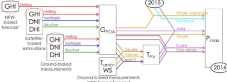
Our approach is similar to indirect forecasts: firstly, we predict solar irradiance and ambient temperature, and then, using a PV performance model of the module, we calculate the PV power produced. The different stages of the PV forecast are summarized in Fig. 1, together with the methods used in this study.

Fig. 1. Schematic of the protocol of PV production forecast and

studied models.

This study focuses on the evaluation of the uncertainty on PV production estimation, step by step, starting from horizontal irradiances and ambient temperature.

The meteorological forecast step is not considered here, even though we know that it may carry the largest part of uncertainty.

The estimation of the uncertainty is done by comparison of calculated and measured values, with different methods of calculations for each step shown in Fig 1.

For this purpose, we firstly present the experimental measurements: atmospheric-related and from a PV-module platform.

In section III we consider diverse models to estimate GPOA,

TPV and PMPP. All models are evaluated against local

measurements at 1-hour time step. All the results are grouped in section IV.

II. EXPERIMENTAL PLATFORMS DESCRIPTION

The experimental platforms are installed at the SIRTA observatory [3] located in Palaiseau (France, 48.7N, 2.2E), on the campus of École Polytechnique (Université Paris-Saclay), 15 km South-East of Paris.

A. Instrumental atmospheric measurements

This study uses two types of atmospheric measurements as input: ground-based measurements and satellite images.

The ground-based measurements are realized at the SIRTA observatory. It is a reference meteorological and climate observatory with more than 150 remote sensing and in-situ instruments. In terms of radiometric measurements, the site is part of the Baseline Surface Radiation Network (BSRN, http://bsrn.awi.de/) since 2003. GHI, DHI and DNI, as well as ground albedo measurements are realized following BSRN standards (with Kipp & Zonen CMP22 and CHP1 radiometers).

This study considers also estimations of GHI, DHI and DNI from Meteosat geostationary satellite observations computed by CAMS [4], [5].

B. Outdoor photovoltaic characterization platform

A test bench PV platform was installed at SIRTA in 2014 and is composed of six commercial PV modules issued from different technologies (Fig. 2). In this paper, we only consider the c-Si PV module (see Table 1).

Fig. 2. Outdoor characterization PV platform located at SIRTA.

The current-voltage characteristics are measured with Agilent DC electronic loads (6060B), each minute from sunrise to sunset. The PMPP is derived from these characteristics. TPV is

measured with 4-wired class A platinum sensors (Pt100) and GPOA is measured with a solar radiometer (Hukseflux NR01)

and a reference PV cell (SOLEMS RG100) installed in the same plane as the PV module.

TABLE I

FRANCEWATTS FL60-250MBPTECHNICAL PARAMETERS

Maximum power PMPP 250 W

Open circuit voltage VOC 37.67 V

Short circuit current ISC 8.64 A

Power temperature coefficient TCP -0.48%/°C

Current temperature coefficient TCI 0.02%/°C

Module area A 1.6285 m²

III. THEORETICAL MODELLING

A. POA irradiance calculation

In this part, the input data used are GHI, DHI and DNI solar irradiances given either by SIRTA ground measurements or by CAMS, as well as the tilt angle and the ground albedo.

The tilt irradiance is calculated using equation (1).

POA POA POA

POA B D A

G    (1)

The beam irradiance is calculated using the DNI as follow:



AOI



cos DNI

BPOA   (2)

The angle of incidence between the sun’s rays and the PV array can be determined as:

   

   





                array , A A tilt z tilt z 1 cos sin sin cos cos cos AOI (3)

where A and z are the solar azimuth and zenith angles,

respectively. tilt and A,array are the tilt and azimuth angles of

the array, respectively.

The albedo arriving in the plane of array is calculated thanks to the fill factor in front of the array:

 

2 cos 1 Albedo GHI A tilt POA      (4)

Albedo corresponds to the coefficient of reflection of the ground and tilt is the tilt angle of the PV module array.

Three models have been considered representing different ways to estimate the diffuse irradiance arriving on PV module:

1) Helbig Model [6]:

The fraction of diffuse irradiance is calculated only from GHI using an empirical relationship, giving an estimated value of DHI and DNI. The diffuse irradiance is then calculated in the same way as described in the isotropic hypothesis.

2) Isotropic hypothesis [7]:

The isotropic sky diffuse model assumes that the diffuse radiation from the sky vault is uniform across the sky. The diffuse irradiance in the plane of array is calculated by equation (5):

 

2 cos 1 DHI D tilt POA     (5)

3) Non isotropic irradiance [8]:

Klucher found that the isotopic model gave good results for overcast skies but underestimates irradiance under clear and partly overcast conditions, when there is increased intensity near the horizon and in the circumsolar region of the sky.

 





 

_                                          z 3 2 tilt 3 tilt POA sin AOI cos GHI DHI 1 1 2 sin GHI DHI 1 1 2 cos 1 DHI D (6)

B. PV module temperature calculation

In this part, we evaluate two models to calculate TPV from

Tamb, GPOA and WS local measurements.

1) Sandia Model [9]:





amb

POA

PV G expa b.WS T

T     (7)

a and b are empirical coefficients establishing the upper limit for module temperature at low wind speeds and high solar irradiance and the rate at which TPV drops as WS increases,

respectively. 2) Faiman Model [10]: .WS U U G T T 1 0 POA amb PV  _ (8)

To evaluate the models, we first consider parameter values proposed by the authors (a = -3.47, b = -0.0594 s.m-1 _{and U}

0 =

25.0 W.m-2_.K-1_{, U}

1 = 6.84 W.m-3.s.K-1). In a second step, we

fit these coefficients to one year of measurements (2015) using the Levenberg-Marquardt method. The obtained coefficients were a = -3.1398, b = -0.305 s.m-1 _{for Sandia}

model and U0 = 21.777 W.m-2.K-1, U1 = 9.855 W.m-3.s.K-1 for

Faiman model.

C. PV power modeling

In this study, we consider six different models to calculate PMPP from the ground-based measurements of GPOA and TPV:

1) Simple model:

It considers a constant CE measured by the manufacturer during a flash test and equal to 0.15086 for our studied PV module.

A G CE

P_MPP _STC _POA (9)

2) Simple improved model:

For this case, the conversion efficiency is taken equal to the average of the measured one during 2015: CE = 0.14339.

3) Evans model [11]:

It takes into account the linear variation of the conversion efficiency with temperature and the low light effect.





                       STC POA 10 STC PV I POA STC MPP G G log γ T T TC 1 A G CE P (10)

With TC1 = 0.0048 from manufacturer data and  = 0.1 deduced from measurement during 2015.

4) Statistical model:

This model does not need internal information from the system to describe its performance. It is a data –driven approach which is able to extract relations on past data to predict the future behavior of the PV module. Here, the past is the year of 2015. Thus, quality of historical data is essential for accurate forecast.

5) One-diode electrical model [12]:

This model is based on the Shockley diode equation, with a current source to model the photo-current (Iph), a single-diode

junction (n is the ideality factor and I0 the saturation current)

and a series resistance (Rs), as shown in Fig. 3.

Fig. 3. One-diode electrical model.

The equation that drives this model is equation (11):





               1 nkT IR V q exp I -I I s 0 ph (11)



I V



max PMPP  (12)

Iph depends on TPV and GPOA, I0 and Rs are temperature

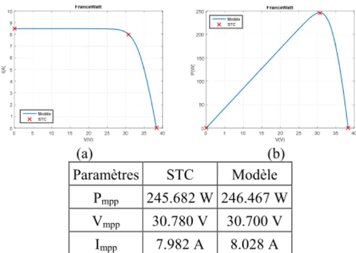
dependent and n is constant. All of the constants used in the above equation are determined by fitting the manufacturer flash test and ratings listed in Table 1, as shown in Fig 4.

(a) (b)

Paramètres STC Modèle

Pmpp 245.682 W 246.467 W

Vmpp 30.780 V 30.700 V

Impp 7.982 A 8.028 A

Fig. 4. Determination of the 4 parameters of the one-diode electrical model by fitting manufacturer data of Table I, I(V) in (a) and P(V) in (b).

6) Artificial neurons network [16]:

The ANN used was built using the feed forward neural network structure with a weighted linear combination and sigmoid function. The architecture chosen is one output (PMPP), three inputs (GPOA, Tamb and WS) and one hidden layer

of five neurons. The training period was the year 2015.

D. Evaluation indicators

In order to compare measurements and calculated values, we compute rMBE and rMAE, as defined in equations (13) and (14).

 

 





 





    N 1 i mpp,meas N 1 i mpp,calc mpp,meas i P i P i P rMBE (13)

 

 

 





    _N 1 i mpp,meas N 1 i mpp,calc mpp,meas i P i P i P rMAE (14)

IV.RESULTS

All presented models in Section II are here evaluated for one independent year of data (2016). Fig. 4 to 6 compare the calculated values to the measured ones. Tables II to IV summarize the rMBE and rMAE obtained results.

A. POA irradiance calculation

In this part, we compare the GPOA calculation methods with

in plane measurements.

(a) (d)

(b) (e)

(c) (f)

Fig. 4. Comparison of the calculated and the measured global irradiance in the plane of array using ground measurements (a), (b) and (c) and satellite estimation (e), (f) and (g). The models are Helbig (a) and (d), isotropic (b) and (e) and Klucher (c) and (f).

The error estimations are summarized in Table II. TABLE II

UNCERTAINTY ESTIMATION IN THE CALCULATION OF GPOA

Input data Model rMBE rMAE

CAMS Helbig 0.160 0.247 Isotropic 0.045 0.189 Klucher 0.078 0.199 SIRTA Helbig 0.001 0.079 Isotropic -0.044 0.074 Klucher -0.018 0.070

Table II shows that all methods using satellite irradiances have a positive bias and absolute error more than double than the results with ground measurements. Isotropic model is the best if data comes from satellite.

B. PV module temperature calculation

The empirical coefficients of the PV module temperature models are first taken as literature values. Then, they were fitted using with the Levenberg-Marquardt method with data from 2015

(a) (c)

(b) (d)

Fig. 5. Comparison of the calculated and the measured PV module temperature using Sandia model (a) and (b) and Faiman model (c) and (d). The empirical coefficient are those found in the literature (a) and (c) and fitted with data of 2015 (b) and (d).

The error estimation is summarized in Table III.

TABLE III

UNCERTAINTY ESTIMATION IN THE CALCULATION OF TPV

Model Coef. from MBE (°C) MAE (°C)

Sandia Literature -0.193 1.883

2015 meas. 0.597 1.364

Faiman Literature 0.485 1.471

2015 meas. 0.647 1.377 Table III shows slightly better results when the model parameters are fitted to the measurements from 2015.

C. PV power modeling

The next figure compare the uncertainty of the model used to simulate the photoelectric effect.

(a) (d)

(b) (e)

(c) (f)

Fig. 6. Comparison of the calculated and the measured PV output maximum power using simple model (a), simple model with CE equal to the average CE of 2015 (d), Evans model (b), satstic model (e), one-diode electrical model (c) and ANN (f).

TABLE IV

UNCERTAINTY ESTIMATION IN THE CALCULATION OF PMPP

Model rMBE rMAE

Simple 0.089 0.094 Improved simple 0.035 0.061 Evans -0.025 0.041 Statistical 0.015 0.045 One-diode 0.034 0.043 ANN 0.0258 0.0425

Table IV shows the improvement of the accuracy of the models, from the simplest to the most complex. A good compromise seems to be the model of Evans.

Interestingly, the lowest rMAE value in the calculated GPOA

(0.070) is 70% larger than for the best PMPP calculation

(4.1%).

V.CONCLUSION

In this paper, we have studied, step by step, the process of the estimation of the PV energy production from GHI, DHI, DNI and Tamb, with a special focus on the calculation of the

uncertainty. Different models have been studied at each step of the calculation.

The next steps will be to show the link between all the models and the error propagation, to consider the step of meteorological and PMPP forecast at different time horizons

and to go through PV plants instead of a unique PV module.

ACKNOWLEDGMENTS

The authors thank the funding from IDEX of Université Paris Saclay, the research program TREND-X from École Polytechnique and the University of Costa-Rica.

GLOSSARY

ANN: Artificial neurons network AOI: Angle Of Incidence

APOA: Albedo in the plan of array (W.m-2)

BPOA: Beam irradiance in the plan of array (W.m-2)

CAMS: Copernicus Atmosphere Monitoring Service CE: Conversion efficiency

DHI: Diffuse horizontal irradiance (W.m-2₎

DNI: Direct normal irradiance (W.m-2₎

DPOA: Diffuse irradiance in the plan of array (W.m-2)

GHI: Global horizontal irradiance (W.m-2₎

GPOA: Plan of array irradiance (W.m-2)

PMPP: Maximum power point (W)

rMAE: Relative mean absolute error rMBE: Relative mean bias error Tamb: Ambient temperature (°C)

TPV: PV module temperature (°C)

WS: Wind speed (m.s-1₎

REFERENCES

[1] EPIA, "Connecting the Sun. Solar photovoltaic on the road to largescale grid integration", 2012.

[2] PV GRID, "Final Project Report", 2014.

[3] Haeffelin, M., et al (2005). SIRTA, "A ground-based atmospheric observatory for cloud and aerosol research". Annales Geophysicae (Vol. 23, No. 2, pp. 253-275).

[4] Z. Qu, A. Oumbe, P. Blanc, B. Espinar, G. Gesell, B. Gschwind, L. Klüser, M. Lefèvre, L. Saboret, M. Schroedter-Homscheidt, and L. Wald L, "Fast radiative transfer parameterisation for assessing the surface solar irradiance: The Heliosat-4 method", Meteorologische Zeitschrift, 2016.

[5] M. Schroedter-Homscheidt A. Arola, N. Killius, M. Lefèvre, L. Saboret, W. Wandji, L. Wald, and E. We Evaluating y, "The Copernicus Atmosphere Monitoring Service (CAMS) Radiation Service in a nutshell", SolarPACES, Abu Dhabi, UAE, 2016. [6] N. Helbig, "Apllication of the radiosity approach to the

radiation balance in complex terrain" Thesis at University of Zurich, 2009. 0 50 100 150 200 250 Measured Pmpp (W) 0 50 100 150 200 250 C a lc u lated P m pp S im p le m odel (W ) 2016 rMBE = 0.089 rMAE = 0.094 0 10 20 30 40 50 60 70 Tpv(°C) 0 50 100 150 200 250 Measured Pmpp (W) 0 50 100 150 200 250 C a lc u lated P m pp S im p le i m proved (W ) 2016 rMBE = 0.035 rMAE = 0.061 0 10 20 30 40 50 60 70 Tpv(°C) 0 50 100 150 200 250 Measured Pmpp (W) 0 50 100 150 200 250 C a lc u lated P m pp E v an s (W ) 2016 rMBE = -0.025 rMAE = 0.041 0 10 20 30 40 50 60 70 Tpv(°C) 0 50 100 150 200 250 Measured Pmpp (W) 0 50 100 150 200 250 C a lc u lated P m pp S tati s ti cal (W ) 2016 rMBE = 0.015 rMAE = 0.045 0 10 20 30 40 50 60 70 Tpv(°C) C a lc ul ated P m pp (W )

[7] H. C. Hottel B. B. Woertz, "Evaluation of flat-plate solar heat collector" Trans. ASME 64, p. 91, 1942.

[8] T. M. Klucher, "Evaluation of models to predict insolation on tilted surfaces", Solar Ener gy ,23 (2), pp. 111-114, 1979. [9] D.L. King, W.E. Boyson, J.A. Kratochvil, "Photovoltaic Array

Performance Model", Sandia National Laboratories, SAND2004-3535, 2004.

[10] D. Faiman, "Assessing the outdoor operating temperature of photovoltaic modules", Prog. Photovolt.: Res. Appl. 16, pp. 307–315, 2008.

[11] D. L. Evans, "Solar energy simplified method for predicting photovoltaic array output", Vol. 27, No. 6, pp. 555-560, 1981 [12] Antonanzas J., Osorio N., Escobar R., Urraca R.,

Martinez-de-Pison F.J., Antonanzas-Torres F., "Review of photovoltaic power forecasting", Solar Energy 136, p. 78 (2016)

[13] Bishop J. W., "Computer simulation of the effects of electrical mismatches in photovoltaic cell interconnection circuits", Solar Cells, 25 (1), p. 73 (1988)

[14] Karamirad, M., Omid, M., Alimardani, R., Mousazadeh, H., Heidari, S.N., "ANN based simulation and experimental verification of analytical 4 and 5 parameters models of PV modules". Simul. Model. Pract. Theory 34, p. 86 (2013) [15] W. R. Geoffrey, " MPPT converter topologies using matlab PV

model", AUPEC: Innovation for Secure Power, Queensland University of Technology, Brisbane, Australia, pp. 138-143, 2000.

[16] A. Mellit., S. A. Kalogirou, "Artificial intelligence techniques for photovoltaic applications: a review". Prog. Energy Combust. Sci. 34, pp. 574–632, 2008.33