Detection of Prostate Cancer using Multi-parametric Magnetic Resonance by
Ian Chan
Submitted to the Department of Electrical Engineering and Computer Science in Partial Fulfillment of the Requirements for the Degrees of
Master of Engineering in Electrical Engineering and Computer Science at the Massachusetts Institute of Technology
August 15, 2002
The author hereby grants to M.I.T. permission to reproduce and distribute publicly paper and electronic copies of this thesis
and to grant others the right to do so
Author
Department of Electrical Engineering and Computes; Science
Certified by __ _ __ _ William___
William Wells ill
, Thesis
Supervisor-Accepted by
Arthur C. Smith Chairman, Department Committee on Graduate Theses
MASSACHUSETTSINSTITUTE OF TECHNOLOGY
BARKER
JUL 3 0 2003
Detection of Prostate Cancer using Multi-parametric Magnetic Resonance
by
Ian Chan Submitted to the
Department of Electrical Engineering and Computer Science August 15, 2002
In Partial Fulfillment of the Requirements for the Degree of
Master of Engineering in Electrical Engineering and Computer Science
ABSTRACT
A multi-channel statistical classifier to detect prostate cancer was developed by combining
information from 3 different MR methodologies: T2-weighted, T2-mapping, and Line Scan Diffusion lmaging(LSDI). From these MR sequences, 4 sets of image intensities were obtained: T2-weighted(T2W) from T2-weighted imaging, Apparent Diffusion Coefficient(ADC) from LSDI, and Proton Density (PD) and T2 (T2Map) from T2-mapping imaging. Manually- segmented tumor labels from a radiologist were validated by biopsy results to serve as tumor "ground truth."
Textural features were derived from the images using co-occurrence matrix and discrete cosine transform. Anatomical location of voxels was described by a cylindrical coordinate system. Statistical jack-knife approach was used to evaluate our classifiers. Single-channel maximum likelihood(ML) classifiers were based on 1 of the 4 basic image intensities. Our multi-channel classifiers: support vector machine (SVM) and fisher linear discriminant(FLD), utilized 5 different sets of derived features. Each classifer generated a summary statistical map that indicated tumor likelihood in the peripheral zone(PZ) of the gland. To assess classifier accuracy, the average areas under the receiver operator characteristic (ROC) curves were compared. Our best FLD classifier achieved an average ROC area of 0.839 (±0.064) and our best SVM classifier achieved an average ROC area of 0.761 (±0.043). The T2W intensity maximum likelihood classifier, our best single-channel classifier, only achieved an average ROC area of 0.599 (± 0.146). Compared to the best single-channel ML classifier, our best multi-channel FLD and SVM classifiers have statistically superior ROC performance with P-values of 0.0003 and 0.0017 respectively from pairwise 2-sided t-test. By integrating information from the multiple images and capturing the textural and anatomical features in tumor areas, the statistical summary maps can potentially improve the accuracy of image-guided prostate biopsy and enable the delivery of localized therapy under image guidance.
PREFACE ... 2
PART 1: TH E EXPERIM ENT ... 2
INTRODUCTION ... 2
M ATERIALS AND M ETHODS ... 4
Patient selection and imaging protocols ... 4
Tumor "ground-truth " labels ... 5
Texturalfeatures ... 5 Anatomicalfeatures ... 6 F e a tu re se ts ... 6 Statistical classifiers ... 6 S of tw a re ... 6 Classifier accuracy ... 6 RESULTS ... 7 Pathology summary ... 7
Signal intensity statistics ... 7
Classifier accuracy ... 8
CONCLUSION S ... 11
PART 2: SOFTW AR E TOOLS ... 17
GETTING STARTED: DOWNLOADING JAVA ... 17
BASIC COMMANDS ... 17
Loading images ... 17
Adjusting Window/Level ... 17
Viewing to a Different Slice ... 18
Im a g e S ize ... 1 8 Scan Information ... 18 Export to M ATLAB ... 18 Export to Slicer ... 18 Configuration ... 19 Closing ImagelExiting ... 19
SEGMENTATION AND REGION OF INTEREST (ROI) ... 19
DrawinglErasinglHiding a ROI ... 19
LoadinglSaving ROI ... 20
Export an ROI to Slicer ... 20
CopyinglSubtracting 2 ROIs ... 20
Biopsy Validated ROI ... 20
IMAGE STATISTICS ... 20
R O I Vo lu m e ... 2 1 Histogram: Image, ROI, Smap Histogram ... 21
Correlation Coefficients and Scatter Plots ... 21
FITTING ONE IMAGE VOLUME INTO ANOTHER: RESAMPLING ... 21
CLASSIFIER TRAINING ... 22
Standardizing Feature ... 22
Build Co-occurrence matrices ... 22
Building Classifiers: FLD and SVM ... 22
SUMMARY STATISTICAL M AP (SMAP) ... 22
Generating a SmaplApplying a Classifier ... 22
Loading a Smap ... 23
Controlling Smap Appearance ... 23
Smap Error RatelROC ... 24
ACK NOW LEDGEM ENTS ... 25
Preface
This thesis consists of two parts. Part 1 describes the experimental methods and results and Part 2 serves as a user manual for the software tools developed for the experiments in part 1. While we are planning to publish the results from part 1 in a research journal, it is my hope that readers will find some documentation in part 2 which can help them develop their own applications for future prostate cancer studies. I also plan to post a web version of the user manual in Part 2 on the internet as well as the accompanying Java and
MATLAB source code. Correspondence and request for source codes should be made by email: [email protected].
Part 1: The Experiment Introduction
Prostate cancer is the most commonly diagnosed non-cutaneous malignancy and the second-leading cause of death from cancer in American men'. Over 40,000 American men are diagnosed with prostate cancer each year and cancer is found at autopsy in 30% of men at the age of 502. 1.5T axial T2-weighted MR prostate images with an endorectal coil enables improved visualization and localization of prostate substructure [central gland(CG) and peripheral zone(PZ)], providing valuable anatomical information because the majority of
prostate cancers develop in the PZ3. While such diagnostic T2-weighted MRI
is a sensitive non-invasive imaging technique for detecting focal abnormalities in the prostate, it lacks specificity for tumor against benign prostatic
hyperplasia(BPH) and other abnormalities. It is reported that T2W MR has a specificity of 43% for nonpalpable tumors and a sensitivity of 85% for
nonpalpable, posteriorly located tumors4. There is a need of integrating
information from other MR methodologies or imaging modalities to improve tumor detection.
Recent advances in MR techniques have allowed us to integrate information based on water diffusion and T2 properties to improve MR specificity for prostate cancer. Quantitative T2-mapping is motivated in part by some intriguing results from Liney et al, which suggest that there is a positive correlation between the concentration of citrate, as determined by IH
spectroscopy, and the water T2 value obtained from T2-mapping methods"'''. Since citrate is the "good" metabolite of the prostate gland, presenting the strongest metabolite signal in normal tissue and BPH', a decrease in the citrate signal provides an indirect indication of potential cancer. If T2-maps indeed correlate with citrate concentrations, i.e. carry the same diagnostic content, the higher spatial resolution of T2-mapping compared to MR spectroscopy would offer potentially greater utility in tumor localization in the prostate.
Diffusion-weighted and quantitative diffusion MR imaging (ADC mapping) is used to obtain tissue contrast reflecting water molecular diffusion. Diffusion MR has become essential for assessing acute stroke in the brain9"0. More recently, evidence has been presented which suggests that diffusion imaging may also play a role in the early detection of tumor response to therapy '.
However, diffusion studies have largely been limited to the brain for a variety of reasons including motion sensitivity and the chemical shift and
susceptibility artifacts which plague single-shot echo planar imaging (EPI) techniques used to overcome motion sensitivity. A diffusion technique with low motion sensitivity and reduced susceptibility and chemical shift artifacts is the so-called line scan diffusion imaging (LSDI) technique recently developed and shown useful for brain and spine imaging. Its primary drawback is slower acquisition times compared to single-shot EPI methods, though full coverage of the rather small prostate gland at reasonable spatial resolutions
(16 mm3 voxels) is readily attained in several minutes. Thus we have used
LSDI methodology to obtain quantitative diffusion data from our patients,
motivated in part by preliminary results of others which suggest reduction of
ADC values in tumor vs normal PZ14.
Earlier works on multi-channel MRI classifier are based on maximum
likelihood5'16. There are also many alternative statistical approaches to multi-channel classification for image analysis and pattern recognition1 7. Fisher linear discriminantlg is a traditional approach where the d-dimensional feature space is projected onto a line which results in the largest variance of the data.
y = w x
where x is the data vector and y is the projected value on a line. w is proportional to:
w
cc
S,'(mt - mn)where Sw = Ytumor (x - mt)(x - mt)T + Enormal (x - m.)(x - mn)T is the pooled sample variance of the two classes and mt and m. are the mean of the tumor and normal samples respectively.
Introduced in 1995 by Vapnik", support vector machine" is a classification technique that has gained popularity in recent years for medical applications". The objective function that SVM maximizes is: LD = i U- 0.5 Zij aiajK(xi,xj)
, subject to 0 cc C and Ei ay = 0. x is the multi-dimensional data vector
and y is the corresponding class label (+1 or -1 for our 2-class problem). i,j = 1.. .L where L = number of training samples. K(x,y) is the kernel function that maps the input to a higher dimensionality and giving the decision boundary its
non-linearity. SVM training yields w, which is given by N i K(yi,xi) where
N is the number of support vectors. A data point xi is a support vector when
the corresponding cxi > 0. Support vectors are sample data points that lie on the decision boundary. One can assign the class label based on y = xT w + b where b is the bias term obtained from SVM training. The more positive y is, the farther x is away from the decision boundary and the more likely it is to be a member of class +1. The case is similar for the -1 labels when y < 0.
To enhance the feature space, many medical image classification applications used machine vision techniques including co-occurrence matrices and various spatial-frequency filters that can enhance image features. Haralick and
Shanmugan pioneered the use of co-occurrence matrix(CM) to capture image texture. A co-occurrence matrix is a probability density distribution of two pixel intensities conditioned on distance and angle between the two pixels.
Recent applications of CM in medical image analysis include MR
T2-weighted breast cancer23, breast mammograms24, MR imaging for tracking
Alzheimer's disease2 5 and coloscopic images of cervix lesions26. The textural
features generated by co-occurrence matrices were reported to enhance classification power in these studies.
We conducted a set of experiments to assess our hypothesis that the SVM classifier performs better than a FLD or a ML classifier. Also, we hypothesize that classifiers that integrate anatomical and textural can achieve a higher tumor detection performance than a classifier based on image intensities alone. Our objective is to construct a summary statistical map based on
multi-parametric MR images that can improve tumor detection and localization. Improved tumor localization will be valuable for a variety of treatment
strategies for prostate cancer including brachytherapy, focused-ultrasound and other image-guided therapies in the future.
MATERIALS AND METHODS
Patient selection and imaging protocols
We enrolled 15 patients who satisfy the eligibility criteria of this study. They were men with abnormal PSA levels ( > 4 ng/ml) and either have had at least 2
prior negative/normal prostate biopsies performed by TRUS or who cannot undergo TRUS biopsies because of prior rectal surgery. In our analysis, we separated the patients into two groups based on whether they underwent brachytherapy because post-brachytherapy patients tended to have altered T2W intensities. We only built multi-channel classifiers for the
non-brachytherapy group because we had a larger number of patients in that group. The 1.5T MR imaging used endorectal coil with an integrated pelvic-phased multicoil array (Signa LX, GE Medical Systems, Milwaukee WI). The endorectal coil is a receive-only coil mounted inside a latex balloon, and assumes a diameter of 4-6 cm once inflated in the patient's rectum). The patient is placed supine in the closed-bore magnet for the examination. The axial T2-weighted images were fast spin echo (FSE) images (4050/135, field of view of 12 cm, section thickness of 3 mm, section gap of 0 mm, matrix of 256x256, 3 signal averages). Typical acquisition times are 5-6 min.
Diffusion-weighted images were obtained with LSDI acquired in an oblique coronal orientation for maximal gland coverage. LSDI involved the use of a pair of slice selective RF pulses to elicit an appropriately diffusion weighted spin echo signal from a single column (loosely referred to as "line" in the
LSDI acronym) of tissue. The LSDI sequence employed 64 columns per slice
with each column being 4 mm2 in cross-section and with a column resolution
of 1.5 mm. Two b-factors, 5 and 750 sec/mm2 were employed along with three
separate diffusion sensitization directions (1,-i,-1/2), (1/2,1,-i) and (1,1/2,1). Though individual columns were sampled every 0.12 s, the effective repetition time (TR) was greater than 4 sec so that minimal TI-weighting occurred. A TE of 70 ms accommodated the high b-factor of 750 sec/mm2 using our available gradient strengths (maxima of 2.3 Gauss/cm). With these sequence parameters, high quality trace ADC maps that combined diffusion coefficient from the 3 orthogonal directions were generated. A total of 5 to 12 slices at 4 mm slice thickness and no gap were used to cover the entire gland with 4 x 4 x 1.5 mm3
voxel dimensions in total scan times between 5 and 10 minutes (50 s/slice).
A Fast Spin Echo (FSE) sequence utilizing 8 echoes with an echo spacing of 13.5 ms was employed to make maps of the spin-spin relaxation time T2
throughout the entire prostate gland at a 3 x 0.7 x 0.8 mm3 spatial resolution. The signal intensity (S) has the approximate form S = p (1- TR/T1)
exp(-T2/TE), where p is the PD intensity, TI the spin-lattice relation time, T2 the spin-spin relaxation time and TR/TE the repetition time/effective echo time combination. A 256 x 192 (frequency by phase) in-plane matrix was used with a 2.5 s TR to gather 5 to 12 three-mm thick contiguous images of the gland in 60s. The sequence is repeated 4 times with 4 different values of the effective echo time ranging from 27 to 108 ms at 27 ms intervals. Thus in
approximately 4 minutes a complete data set is collected that allows for mapping the T2 value throughout the gland by performing mono-exponential fits of signal intensity vs echo time for each voxel. The y-intercept of the fits is the Proton Density (PD) intensity and the negative inverse of the slope is the pure T2 value used for the T2Map intensities.
Tumor "ground-truth" labels
A radiologist manually outlined suspected tumor(TU), peripheral zone(PZ),
and total gland (TG) on axial T2-weighted images, which are used in clinical diagnosis. We combined the tumor label with sextant biopsy pathology
reports to form biopsy validated tumor labels for classifier training. In sextant biopsy, the PZ is divided into 6 regions: left/right + base/mid/apex. Only regions marked positive for cancer in both the biopsy report and the radiologist's label are included in the validated tumor labels.
Textural features
It is observed that tumor textures in the prostate possess radial symmetry, we eliminated the angle(0) dependence in the occurrence matrices. Our co-occurrence matrix covered a 9x9 pixel window and had 14 distinct distances. We scaled image intensities to fit a range between 0-255 by mapping the 256 levels linearly onto the image intensity range of max{0, (p-3.a)} to (p+3.). For each center pixel, we considered its n neighbors that were equi-distant from the center pixel. We constructed log likelihoods (log
(P(tumor)/P(normal)) for each of these n pairs and took the median of the n log likelihoods as the feature statistic. Because radiologists often considered the slice above or below the current image slice for clues of tumor, we extended the co-occurrence matrix to 3D by constructing co-occurrence matrices one slice above and below the current slice. 14 features for the CM from the same slice and 15 features from the CM one slice above or below the center pixel resulted in 29 CM features total for each of the four basic MR images.
To capture the frequency characteristics of tumor, we computed discrete
cosine transform(DCT)27 using a 7pixel x 7 pixel window. The 49 DCT
Anatomical features
We used the cylindrical coordinate system(r, 0,z) to describe each anatomical location and set the origin at the centroid of the gland. r and z are rescaled to
fit the range of -1 to 1 for each gland. 0 is in the range of 0 to n with anterior set to 0 and we assume left/right symmetry of the gland. The z coordinate could help distinguish the apex, mid-gland, and base, which had observably different image and anatomical features. Empirical observations pointed to common occurrences of prostate tumors in the axial 5:00 and 7:00 o'clock positions of the PZ and the 0 coordinate could potentially distinguish these
anatomical areas.
Feature sets
5 feature sets were chosen to test our classifiers. basic 4 includes only the four
signal intensities: T2W, ADC, PD and T2Map. basic 4+anatomy includes the 4 signal intensities and the 3 cylindrical coordinates from anatomical features. Besides the 7 features in basic4+anatomy, al/CM also includes 29
co-occurrence matrix entries for each MR sequence, generating an additional 4x29 features. allDCT includes all the basic4+anatomy features plus the DCT features from all 4 types of MR images. allCM+DCT is the union of all the features in al/CM and allDCT.
Statistical classifiers
For this study, we randomly sampled 30% of the PZ data and retained all the tumor data because we had about 20 times more PZ data than tumor data. All
features were standardized to pt = 0 and a = 1 prior to training. After
obtaining the FLD vector w, we constructed a maximum likelihood classifier using the training dataset.
For SVM training, we randomly sampled 10% of the PZ data and retained all the tumor data to confine the training dataset to a reasonable size for SVM training convergence. All features are standardized to p = 0 and cY = 1 prior to training. We chose the radial basis function kernel K(x,y) = exp {-Ix-yj2
/G}
with parameters a = 2 and C = 100. In this study, we used the MATLAB
support vector toolbox28 developed by Crawley, which used Platt's sequential
minimization algorithm for optimization29.
Software
All feature generation and classifier training were computed using the
MATLAB software package. The software for manual segmentation by the radiologist, volume calculation and image interpolation was developed in-house for this project with the Java language.
Classifier accuracy
To compare the accuracy of classifiers, we performed standard Receiver Operator Characteristics (ROC)3 analysis on each of the 11
non-brachytherapy patients. We chose the area under the ROC curve as our
benchmark for classifier performance. We adopted a jack-knife strategy where we trained the classifier with n-I cases and applied the trained classifier on the remaining case. The pt ± a of the n leave-one-out ROC areas were reported.
To determine the significance in the difference in mean ROC areas of two classifiers, we utilized pairwise 2-sided students' t-test at cx=0.05.
RESULTS
Pathology summary
We divided the patients into two groups: post-brachytherapy and non-brachytherapy. Of the 11 non-brachytherapy patients in this study, 9 had
confirmed adenocarcinoma and 1 had prostatic intraepithelial neoplasm(PIN), a precursor to cancer, from the biopsy reports. The average tumor volume was
1.03±0.56cm3 and the average total gland volume was 43.03±19.26cm3. The
mean percentage of tumor volume/PZ volume was 6.80±3.99%. Patients in this group had small to medium size tumors, with minimal seminal vesicle and extra-capsule invasion. The average Gleason score for those with confirmed cancer was 6.2 and had a range of 6-7, indicating that most of the non-brachytherapy patients had medium grade adenocarcinoma. Of the 4 post-brachytherapy patients in this study, the average tumor volume was
1.72±1.50cm3 and the average total gland volume was 33.36±7.26cm3. The mean percentage of tumor volume/PZ volume was 17.62±18.16%. The average Gleason score for this group was 6.5 and had a range of 6-8, indicating that the patients in this study had medium to high grade adenocarcinoma and had larger tumors.
Signal intensity statistics
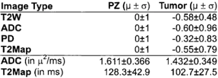
The p. ± a of the signal intensities for each MR image parameter in this study is shown in table 1 and 2. For each patient, PZ intensities were standardized to p = 0 and a = 1 and tumor intensities were standardized using the mean and standard deviation of the PZ for comparison.
Image Type PZ (p ± a) Tumor (p ± a)
T2W 0±1 -0.58±0.48
ADC 0±1 -0.60±0.96
PD 0±1 -0.32±0.83
T2Map 0±1 -0.55±0.79
ADC (in pI/ms) 1.611±0.366 1.432±0.349 T2Map (in ms) 128.3±42.9 102.7±27.5
Table 1 Signal intensity summary for 11 non-brachytherapy patients. PZ signals are standardized to 0 mean and I std dev. Tumor signals are normalized with the mean and standard deviation of the PZ for comparison. Mean and std dev of non-standardized ADC and T2Map values are also presented.
Image Type PZ (p ± a) Tumor (p ± a) T2W 0±1 -0.04±0.89 ADC 0±1 -0.60±0.83 PD 0±1 0.30±1.19 T2Map 0±1 -0.49±0.71 ADC (in pt/ms) 1.524±0.306 1.250±0.314 T2Map (in ms) 88.0±20.7 76.6±15.9
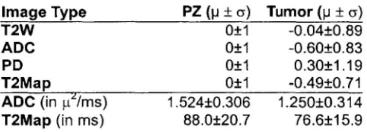
Table 2 Signal intensity summary for 4 post-brachytherapy patients. PZ signals are standardized to 0 mean and 1 std dev. Tumor signals are normalized with the mean and standard deviation of the PZ for comparison. Mean and std dev of non-standardized ADC and T2Map values are also presented.
Classifier accuracy
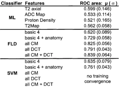
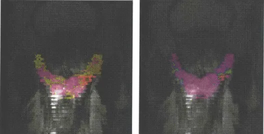
Figure 2 shows two sample summary statistical maps generated by FLD and SVM classifier and figure 3 shows several ROC curves for our best ML classifier and our best multi-channel classifier for 5 patients. The results for the 1-channel maximum likelihood (ML) classifiers, multi-channel Fisher Linear Discriminant Classifiers (FLD) and Support Vector Machine classifiers (SVM) are shown in table 3. Pairwise 2-sided t-tests with c = 0.05 among the
four 1-channel classifiers supported the hypothesis that all 1 -channel classifiers based on intensity alone had statistically equivalent ROC performance (P-values > 0.05).
We compared the multi-channel FLD classifiers with T2 axial ML classifier, the best of the four 1-channel classifiers. Pairwise 2-sided t-tests with Oc = 0.05
supported that FLD with basic 4+anatomy (P-value = 0.0024), all CM
(P-value = 0.0004), all DCT (P-value = 0.002), and allCM+DCT (P-value =
0.0003) offered greater classification power than ML classifier based on T2
axial intensity alone. However, pairwise 2-sided t-tests with cc = 0.05 did not
support that FLD with basic4 classifier performed better than 1-channel T2 axial ML classifier (P-value = 0.355). Similarly, we compared the multi-channel SVM classifiers with T2 axial ML classifier. Pairwise 2-sided t-tests
with c = 0.05 supported that SVM with basic 4+anatomy (P-value = 0.0017)
offered greater classification power than ML classifier based on T2 axial intensity alone. However, pairwise 2-sided t-tests with c = 0.05 did not
support that SVM with basic4 classifier performed better than 1-channel T2 axial ML classifier (P-value = 0.483).
For SVM training, we failed to get convergence for the feature sets allCM,
allDCT and allCM+DCT after 72 hours of simulation. For the other 3 feature
sets basic4 and basic4+anatomy that we managed to get convergence, we
compared the average area under ROC of SVM classifier with FLD classifier using 2-sided pairwise t-test at a = 0.05. SVM performs better than FLD for
basic4+anatomy (P-value = 0.0003) while SVM and FLD have equal
Classifier Features ROC area: p ( a) T2 axial 0.599 (0.146) ML ADC Map 0.533 (0.114) Proton Density 0.521 (0.165) T2Map 0.562 (0.058) basic 4 0.620 (0.089) basic 4 + anatomy 0.729 (0.058) FLD all CM 0.825 (0.056) all DCT 0.791 (0.043) all CM + DCT 0.839 (0.064) basic 4 0.635 (0.079) basic 4 + anatomy 0.761 (0.043) SVM all CM all DCT no training all CM + DCT convergence
Table 3 Summary of Maximum Likelihood (ML), Fisher Linear Discriminant (FLD) and Support Vector Machine (SVM) classifiers results of 10 non-brachytherapy patients. Mean(std dev) of area under ROC of each classifier are presented. T2 axial, ADC Map, Proton Density and T2Map are the 4 basic image intensities and the classifiers for these 1-channel cases are based on maximum likelihood. "basic4" consists of the 4 basic image intensities. "basic4+anatomy" consists of the 4 basic image intensities and the 3 cylindrical coordinates that describe anatomical location relative to the centroid of the prostate. "all DCT" consists of all 4 basic intensities, anatomical information, and frequency transform statistics for all 4 basic images. "all CM" consists of all 4 basic intensities, anatomical information, and co-occurrence statistics for all 4 basic images. "all CM+DCT" consists of all intensity, co-occurrence, anatomical and frequency features.
DISCUSSION
Students' t-test comparisons of ROC areas suggested that SVM produced greater detection power than FLD classifiers for the feature sets al/CM and basic4+anatomy and statistically equivalent detection power for the basic4
feature set. The merits of the nonlinear decision boundary of the SVM classifier become noticeable when the number of features increases.
Although SVM achieved a better performance than FLD, classifier training convergence and simulation time are two issues to consider. The training time for FLD classifiers is generally between 1 to 6 hours and for SVM classifiers between 2 to 60 hours, depending on number of classification channels and the number of samples. We included all tumor samples from the 9 cases for
training (approx. 2500 voxels) and 10% of healthy PZ samples (approx. 5000 voxels). We failed to get convergence on SVM training after 72 hours for the
larger feature sets allCM+DCT and allDCT. This is because both of these feature sets include over 150 channels. The FLD results suggest that feature sets al/CM and allCM+DCT have statistically equivalent performance and therefore, we expected similar findings for SVM had the allCM+DCT training
converged. To include both frequency and CM features, we could have randomly selected a smaller number of CM entries and DCT frequencies to
reduce the dimensionality of the problem as many CM entries and DCT frequencies contain high mutual information.
Utilization of co-occurrence matrix and DCT significantly enhanced tumor features in the images as supported by t-test analysis. For both FLD and SVM classifiers, we noticed that allCM, allDCT and allCM+DCT performed better
than basic4 and basic4+anatomy feature sets according to the ROC area
analysis, which proved the effectiveness of these machine vision techniques for prostate cancer detection with MRI.
We found that the group of patients who underwent brachytherapy had different T2W signal intensity properties compared to the group without brachytherapy. The results in Table 1 and 2 showed that the
post-brachytherapy patients almost had no difference in mean T2W signal intensity between PZ and tumor tissues while for the non-brachytherapy patients, the difference in standardized means of T2W signal intensities between PZ and tumor tissues is 0.58. From the T2W images of post-brachytherapy patients, one can observe that the PZ intensity is darkened as a result of brachytherapy and therefore, it is difficult to differentiate between tumor and PZ tissues based on T2W intensity level.
From the results of the single-channel maximum likelihood (ML) classifiers in Table 3, one may draw the conclusion that the T2-weighted axial images is most informative about differentiating prostate tumor out of the four signal intensities, with the largest average ROC area of 0.599. Yet, we found that the 4 image intensities are equally informative about tumor statistically. Another explanation for the slightly larger ROC area with T2W is that we obtained "ground truth" tumor label with a radiologist contouring axial T2-weighted images. This can introduce bias even though the "ground truth" label is confirmed by biopsy reports. Furthermore, the radiologist examined the axial T2W images, which are at a higher spatial resolution than the LSDI and T2Map images. Therefore, it can be self-serving that we found the T2W images to be most informative about tumor when we defined the "ground truth" tumor regions by expert examination of these images. However, this limitation is difficult to avoid because we had no access to the "ground truth." Confirming the radiologist's "ground truth" label with biopsy reports partially remedied this bias.
The average ROC results show that both SVM and FLD classifiers with basic 4 feature set did not perform better than the best single-channel ML classifier based on T2W intensities according to t-test analysis. However, it is not valid to conclude that LSDI and T2Map did not add any useful information.
Although not statistically significant, we notice that the average ROC area for the ML T2W classifier is 0.599, which is less than 0.620 and 0.635 of the FLD
basic 4 and SVM basic 4 respectively. Further studies need to be done to
compare the textural information in PD, ADC and T2Map images and their mutual information with the textural features in T2W images.
T2W intensities in the PZ near the rectum were corrupted by sharp near-field endorectal coil artifacts. This largely limited the tumor detection ability of the T2W images for PZ tissues near the coil. Advances in intensity correction
methodologies may remove the coil artifacts, which can dramatically improve the quality of T2W images and boost classifier performance.
We adopted a jack-knife strategy when performing classifier assessment because we only had 10 patients with pathologically confirmed tumor in the non-brachytherapy group. As we collected more multi-parametric cases, we could divide patients into two separate groups for classifier training and validation. A larger number of patients could provide image samples that covered a broader spectrum of focal abnormalities and cancer.
In general, we found that adding textural and anatomical information increases the accuracy of three all classifiers used in this study. We also found that SVM is the best of the three classification techniques when the number of features increases. Both observations are consistent with our hypotheses.
CONCLUSIONS
For the purposes of the prostate group at the Surgical Planning Laboratory at the Brigham and Women's Hospital, we will use the statistical summary map to plan MR guided biopsy. In many hospitals, prostate cancer is diagnosed by transrectal ultrasound (TRUS) guided needle biopsy, prompted by either an elevated prostate-specific serum antigen (PSA) level or a palpable nodule from a digital rectal exam (DRE). TRUS biopsy does not target lesions, rather it uses a sextant approach, attempting to sample six representative locations in the gland. This method is limited by its inability to accurately detect, localize and characterize focal tumors in the gland. It suffers from a 8-30% failure rate to detect lesions, which are palpable on DRE313 2. TRUS biopsy is also limited
by low sensitivity of 60% with only 25% positive predictive value A
randomized study of the efficacy of 6 versus 12 biopsy samples showed no difference in cancer detection33. This suggests that the problem is not solved
by simply increasing the number of biopsy samples. In the face of high PSA
levels, the limitations of current biopsy methods are substantial and our project is aimed at addressing these issues.
Integrating information from multiple images and enhancing prostate tumor features in these images are two main objectives in this study. We have demonstrated the utility of two multi-channel classifiers with feature
enhancements using machine vision techniques for prostate cancer detection. We have also shown that our classifiers have statistically superior performance over single-channel intensity-based classifiers. The summary statistical map generated by our classifiers allows radiologists to visualize the high volume of image data and provides summarized pre-operative information for intra-operative procedures. The summary statistical map has the potential of improving biopsy accuracy and enhancing tumor target identification for the delivery of localized therapies.
a) T2-weighted resampled
c) T2 Map d) Proton Density
Fig 1 A sample set of multi-parametric MR images in the oblique coronal plane. Figure (a) is a T2-weighted image, resampled from the axial planes to the oblique coronal planes of the other images. Figure (b) is an ADC Map from LSDI. Figure (c) and (d) are T2 Map and Proton Density images from T2 mapping. The green label is total gland, the yellow label is PZ and the pink label is biopsy validated tumor label.
b) Support Vector Machine -basic4 + anatomy
Fig 2 Summary statistical maps of a) Fisher Linear Discriminant classifier and b) Support Vector Machine classifier. The FLD classifier utilizes all
co-occurrence, DCT, anatomical and signal intensity features and the SVM classifier utilizes signal intensity and anatomical features only. The statistical maps are superimposed on the T2-weighted axial images of the patient in Fig
1 and the magenta label indicates the biopsy-validated tumor region identical to Fig 1. The statistical maps use the rainbow color scheme with red indicating high tumor likelihood and purple indicating low tumor likelihood. One can observe that both statistical maps correctly pick out the tumor area by shading it with red and other non-tumor areas purple. Also, the FLD classifier paints most of the tumor region red whereas the SVM classifier gives weaker results with part of the tumor region painted green and yellow.
4V a 1-1
0.2
0 0.1 ' 03 .4. 062 06 . 7 O S. I
Trsfodftve
Fig 3 Sample ROC curves for 5 different patients. The series of red curves are from the single-channel T2W Maximum Likelihood (ML) classifier and the series of green curves are from the Fisher Linear Discriminant (FLD)
aIICM+DCT classifier. Although ROC curves can be processed to be convex
and above the diagonal by randomized decisions, these sets of ROCs are derived from empirical data without processing.
16000 1400 12000 1600-- -400: SozW: MD 66 500 1000 160D 200 2500 3000 5soo
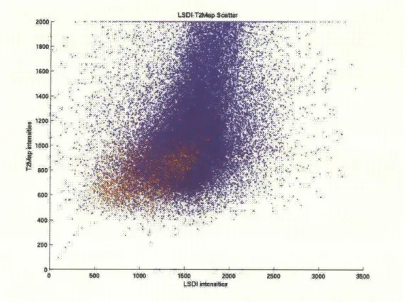
Fig 4 Scatter plot of raw T2map and ADC values from 10 patients. Red
samples belong to tumor tissues and blue samples belong to healthy PZ tissues. One can see that there is an overlap region for the two classes which makes intensity-based classifier non-ideal.
0. 14: :0.I A06:-0 .A06:-04 4,02 A. 0 so. ....CM ~#flCM~~~ 0 10 20 30 40 50 basic4 + anat 0 0. 10 : 0 40 W0 :0 0.2 015 0,1..
AAJ
M
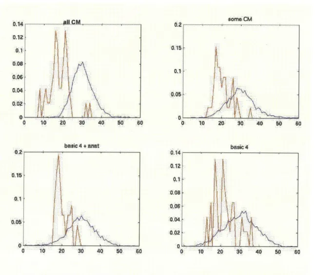
U. .014. 012 C basic 4 1io ao 30o 40 50Fig 5 Probability density functions of tumor(red) and healthy PZ(blue) data
from line-projected data of the Fisher Linear Discriminant classifiers. The more co-occurrence matrix features are included in the classifier, the better the discrimination between the two classes.
A.05(
60
Part 2: Software Tools
Getting started: Downloading Java
The first thing to do is to download the Java software from http://java.sun.com for your appropriate platform. You can compile the source code with the commands
javac -classpath .App Window.java
and run the program with
Java App Window -Xms 128m -Xmxl28m .
The parameters that follow -X specify the minimum and maximum stack size.
Application Consolel
After executing AppWindow, the main window pops up. You can now load images or perform statistical analysis on the images by choosing the available options in the menu bar. Messages in this window will inform you of any errors or messages. Be sure to make appropriate configurations the first time you use the software! (see Configure section) The following sections discuss how to perform different tasks with this software.
Basic Commands Loading images
You can choose File and Load T2, Ti, LSDI or T2Map and a file dialog box will appear. You can click on any of the files of the image series (i.e. 1.001)
and click OK. The program will prompt you to select the range of slices you want to load or the complete volume. Make the appropriate selection and the
images will be loaded.
Adjusting Window/Level
In the opened image window, select Adjust and then Window/Level. You will see a control panel. Move the sliders or type in the desired window and level.
Apply All to apply the current window/level to all slices in the volume.
Viewing to a Different Slice
You can use the up/down arrow or page up/down to traverse the volume and view different slices.
Image Size
You can adjust the size of the image by dragging the corners of the image window.
Scan Information
Choose Info and then Scan Info to see some of the information stored in the image header such as Patient Name, Patient ID and date of Scan.
Export to MATLAB
Choose Export and then Export Images to Matlab from the image window to export the current image volume to Matlab format. The data will be stored in a
256x256 matrix in ASCII text so that it can be opened by the Matlab command load -asciifilename.
Export to Slicer
Choose File and Export to Slicer to save the current image volume to the 3D Slicer format. You will be prompted to provide an image file that contains the appropriate Slicer header information.
Configuration
The user needs to provide some configuration information. such as Matlab pathname for the program to run correctly. Choose from the main window
Options, Configure. The following dialog box will appear. Fill in the appropriate information about directories and constants. You can use the following settings in the figure as reference.
TL ABPath xterm -geometry 1 0A 0+10-10 -e /mitimatlabiarchli386 _inux22/binfmatlab
TiApU~fPl h -Safslathenamiteduluseril/aiianchanbwhfmatlab/
, VF s th jlafsfathena mit eduluserlilarianchanibwhttempl
aximmnummr o imgespr voume 60
axmu itmst L - 30000
umberof piels pr imae (25x25t I6 6 -6553~6
axiumnnnr o wmo 50
Closing Image/Exiting
You can choose Close or Exit from the File menu in the main window and image window to quit.
Segmentation and Region of Interest (ROI) Drawing/Erasing/Hiding a ROI
Choose Segmentation and Manual Draw and the segmentation panel will
appear. Choose the color you want to draw with and you can draw on the image window. There is also auto connect and you can click on various locations and a line will be drawn to connect the points. Click Apply or press Enter to complete the ROI. You cannot move between slices when drawing an ROI.
To erase, click the Clear button in the panel and the entire ROI in this current image will be erased. To hide a ROI, check the Hide box and the ROI will disappear.
Loading/Saving ROI
Select File from the image window and choose Load labelmap and Save labelmap to load and save a ROI.
Export an ROI to Slicer
Slicer saves label map with no header but requires a header when loading a label map. Choose Export, Export ROI to paste a header to a ROI so that Slicer can open it.
Copying/Subtracting 2 ROIs
To copy an ROI from one image to another, choose ROI from the main window and Copy ROI to. A dialog box will prompt you to select the source and destination image windows and the ROI you want to copy. You can also subtract ROI A from ROI B to generate ROI C by choosing ROI and Subtract ROI from the main window.
Biopsy Validated ROI
To combine information from a biopsy report and confirm the presence of tumor in an ROT, choose ROI and Make Pathology Validated Labelmap. The dialog box will prompt you to enter the sextant biopsy results and ask you for a destination filename for the validated labelmap.
~~1LIU~]~j - J L 1L1Zll
ROI Volume
Choose ROI Stat and ROI Volume from the image window. Then select the appropriate ROI and a dialog with the ROI volume in cm3 will appear. The method uses an averaging of 2 neighboring slice areas and multiply the average by the slice thickness to interpolate the volume.
Histogram: Image, ROI, Smap Histogram
Histograms for the pixel values within the ROI or the summary statistical map values within the ROI can be displayed by choosing ROI Stat and ROI
Histogram/ROISmap Histogram. Histogram of intensities can also be generated by choosing Image Stat and Histogram from the image window.
Correlation Coefficients and Scatter Plots
Correlation coefficients of the same ROI in 2 images can be found by
choosing Multi Stat, Correlation Coefficient from the main window. You can also get a scatter plot from Multi Stat, 2D Scatter Plot to generate a scatter plot similar to Figure 4. However, please ensure that the ROI is the same in the 2 images by using a Copy ROI to command. Also, the 2 images need to be
taken in the same plane for this to work.
Fitting one image volume into another: Resampling
When one image volume is scanned in an axial plane and another volume is scanned in a coronal plane for example, we need to resample one of the image volumes into the other by interpolation and linear transformation. Choose Registration, Resample and choose the source and destination image volumes.
A new image volume will be generated and will match the lattice of the
Classifier Training Standardizing Feature
Before training the classifiers, we need to find the mean and standard
deviation of all the features so that we can perform normalization. To do that,
choose Training, Standardize Features from the main window. It will ask you
for 1) the path for the text file that stores the directories of the patient scans, the co-occurrence matrix data file, the feature output file and the pmem, or the fraction of data to sample. Entering 0.5 here means sampling half the data to find the mean/std dev.
Build Co-occurrence matrices
To build the co-occurrence matrices for the images, choose Training, Build Co-occur. Matrix from the main window. It will prompt you for the patient directory location file and the output file for the CM data.
Building Classifiers: FLD and SVM
From the Training menu in the main window, choose the appropriate classifier from the sub-menu and a dialog will prompt you for the file locations,
including the patient directory location file, the Co-occurrence matrix output file, the standardized feature file, etc. Matlab will start and simulations will begin. Do no close the Matlab window as this will terminate the classifier training.
Summary Statistical Map (Smap)
Generating a Smap/Applying a Classifier
From the main window, choose Stat Map and Apply FLD or Apply SVM to apply the trained classifier to a specific case. Fill in the appropriate image location directories for the particular case in the dialog provided. You can click on Browse to search for the filenames.
Loading a Smap
From an image window, choose Stat Map, Load Smap. A dialog will prompt you for the smap location. You can load up to 3 Smap's in the same image window.
Controlling Smap Appearance
After loading the Smap, choose Stat Map, Appearance and Threshold to open the Smap adjustment panel to change the bounds and transparency of the Smap. To get a histogram of the distribution of the Smap values, click Histo from the panel. The hide checkbox toggles the Smap appearance in the image window.
Displaying Image #: 6 ofi 2 LSDI TRACE'
Smap Error Rate/ ROC
To find the area under the Receiver Operator Characteristic Curve and plotting the ROC, choose Stat Map, Smap Error Rate from the image window.
Matlab will be invoked and the ROC for the chose classifier and Smap will be plotted.
ACKNOWLEDGEMENTS
I want to thank my father, who was a cancer patient and who always inspired
me to learn and enjoy learning. His spirit is my motivation behind this project on cancer diagnostics because I hope that my research can directly benefit other cancer patients.
I want to thank Dr. Clare Tempany from the Brigham and Women's Hospital
for her mentorship. I am grateful for the opportunity of working at the Surgical Planning Laboratory. I will always be amazed by the number of things she can do at a time.
I am also very grateful to William (Sandy) Wells, who is always supportive
and resourceful. He can always provide me with insight when I am stuck, and with calmness when I start to panic.
I am also very thankful to Monique, who puts up with me even when I become
unreasonable. Getting to meet her is my most delightful MIT experience.
References
I "Cancer facts and figures," American Cancer Society, Atlanta Georgia 1997.
2 L. Garfinkel and M. Mushinski, "Cancer incidence, mortality, and survival trends in four leading sites," Stat. Bull. 75, 19-27 (1994).
3 D. Cheng and C. Tempany, "MR imaging of the prostate and bladder," Semin Ultrasound CT MR 19, 67-89 (1998).
4 H. Carter, R. Brem, C. Tempany, A. Yang, J. Epstein, P. Walsh, E. Zerhouni, "Nonpalpable prostate cancer: detection with MR imaging," Radiology 178, 523-525 (1991)
5 G. Liney, L. Turnbull, M. Lowry, L. Turnbull, A. Knowles, A Horsman, "In vivo quantitation of citrate
concentration and water T2 relaxation time of the pathologic prostate gland using 1 H MRS and MRI," Magn Reson Imag 15,1177-1186 (1997).
6 G. Liney, M. Lowry, L. Turnbull, D. Manton, A. Knowles, S. Blackband, A. Horsman, "Proton MR T2 maps correlate with the citrate concentration in the prostate," NMR in Biomed. 9, 59-64 (1996).
7 G. Liney, A. Knowles, D. Manton, L. Turnbull, S. Blackband, A. Horsman, "Comparison of conventional single echo and multi-echo sequences with a fast spin-echo sequence for quantitative T2-mapping: Application to the prostate," J Magn Reson Imag 6, 603-607 (1996).
8 J. Garcia-Segura, M. Sanchez-Chapado, C. lbarburen, J. Viano, J. Angulo, J. Gonzalez, J. Rodriguez-Vallejo, "In vivo proton spectroscopy of diseased prostate: Spectroscopic features of malignant versus benign pathology," Magn.
Reson. Imag. 17, 755-765 (1999).
9 P. Schaefer, P. Ellen Grant, R. Gilberto Gonzalez, "Diffusion-weighted MR imaging of the brain," Radiology 217, 331-345 (2000).
10 R. Gonzalez, P. Schaefer, F. Buonanno, L. Schwamm, R. Budzik, G. Rordorf, B. Wang, A. Sorensen, W. Koroshetz, "Diffusion-weighted MR imaging: Diagnostic accuracy in patients imaged within 6 hours of stroke symptom onset," Radiology 210, 155-162 (1999).
11 T. Chenevert, L. Stegman, J. Taylor, P. Robertson, H. Greenberg, A. Rehemtulla, B. Ross, " Diffusion magnetic resonance imaging: an early surrogate marker of therapeutic efficacy in brain tumors. J Natl Cancer Inst
92:2029-2036; 2000.
12 M. Zhao, J. Pipe, J. Bonnett, J. Evelhoch, "Early detection of treatment response by diffusion-weighted 1 H-NMR spectroscopy in a murine tumour in vivo," Br J Cancer 73, 61-64 (1996).
13 R. Robertson, S. Maier, R. Mulkern, S. Vajapeyam, C. Robson, P. Barnes, "MR line-scan diffusion imaging of the spinal cord in children," AJNR 21, 1344-1348 (2000)
14 B. Issa, "In vivo measurement of the apparent diffusion coefficient in normal and malignant prostatic tissues using echo-planar imaging," JMRI 16, 196-200 (2002)
15 M. Vannier, R. Butterfield, D. Rickman, D. Jordan, W. Murphy, P. Biondetti, "Multispectral magnetic resonance image analysis," Radiology 154, 221-224 (1985)
16 H. Cline, E. Lorensen, R. Kikinis, F. Jolesz, "Three-dimensional segmentation of MR images of the head using probability and connectivity," J Comput Assist Tomogr 14(6), 1037-1045 (1990)
17 R. Duda, P. Hart, Pattern Classification and Scene Analysis, (John Wiley, New York, 1973).
18 C. Bishop, Neural Networks for Pattern Recognition, (Clarendon Press, 1995)
19 V. Vapnik, The Nature of Statistical Learning Theory. (Springer 1995)
20 C. Burges, "A Tutorial on Support Vector Machines for Pattern Recognition. Data Mining and Knowledge Discovery," 2(2), 121-167 (1998)
21 P. Golland et al, "Small Sample Size Learning for Shape Analysis of Anatomical Structures," In Proc. Of MICCAI' 2000, LNCS 1935, 72-82 (2000).
22 R. Haralick, K. Shanmugan, I. Dinstein, "Texture for image classification," IEEE Transactions on Systems, Man, and Cybernetics 3(6), 610-621 Nov (1973)
23 G. Torheim et al, "Feature Extraction and Classification of Dynamic Contrast-Enhanced T2-Weighted Breast Image Data IEEE Trans Medical Imaging," 20, 12 December (2001)
24 J. Kim, H. Park, "Statistical Texture Features for Detection of Microcalcifications in Digitized Mammograms," IEEE Trans Medical Imaging 18, 3 March (1999)
25 P. Freeborough, N. Fox. "MR Image Texture Analysis Applied to the Diagnostic and Tracking of Alzheimer's Disease," IEEE Trans Medical Imaging 17, No 3 June (1998)
26 J. Qiang, E. Craine, "Texture Analysis for Classification of Cervix Lesions," IEEE Trans. on Medical Imaging 19,
II November (2000)
27 A.Oppenheim, R. Schafer, Discrete-Time Signal Processing, (Prentice Hall, Englewood Cliffs, New Jersey, 989)
28 G. Cawley. MATLAB Support Vector Machine Toolbox vO.50 http://theoval.sys.uea.ac.ukA-gcc/svm/toolbox University of East Anglia (2000)
29 J. Platt, "Fast training of support vector machines using sequential minimal optimization, in Advances in Kernel Methods -Support Vector Learning," (Eds) B. Scholkopf, C. Burges, and A. Smola, (MIT Press, Cambridge, MA, chapter 12, pp 185-208, 1999).
30 C. Metz, "ROC methodology in radiologic imaging," Invest Radiolo 21, 720-733 (1986)
31 J. Kurhanewicz, R. Dahiya, J.M. Macdonald, L. Hong Chang, T.L. James, P. Narayan, Citrate alterations in primary and metastatic human prostatic adenocarcinomas: I H magnetic resonance spectroscopy and biochemical study, Magn. Reson. Med. 29, 149-157 (1993).
32 M Schiebler, K Miyamoto, M. White, S Maygarden, J Mohler, In vitro high resolution I H spectroscopy of the human prostate: benign prostatic hyperplasia, normal peripheral zone and adenocarcinoma, Magn. Reson. Med. 29, 285-291 (1993).
33 J Kurhanewicz, D Vigneron, H Hricak, P Narayan, P Carroll, S Nelson, Three-dimensional H-1 MR spectroscopic imaging of the in situ human prostate with high (0.24-0.7-cm3) spatial resolution. Radiology, 198, 795-805, 1996