Detection of fracture oreientation using azimuthal variation of P-wave AVO responses

Detection of Fracture Orientation Using Azimuthal Variation

of P-wave AVO Responses

by

Maria Auxiliadora Perez

Submitted to the Department of Earth, Atmospheric, and Planetary Sciences

in partial fulfillment of the requirements for the degree of

Master of Science

at the

MASSACHUSETTS INSTITUTE OF TECHNOLOGY

January 1997

DJ

©

1997

MASSACHUSETTS INSTITUTE OF TECHNOLOGY

Signature of Author ...

DeIartment of Earth, Atmospheric, and Planetary Sciences January 17, 1997

Certified by ... ... . . .. .. . .. . . . ..

Professor M. Nafi Toks6z Director, Earth Resources Laboratory Thesis Advisor

Accepted by....

f NV)

F, E 197 U rt;J

Professor Thomas H. Jordan Department Head

Institute Archives and Special Collections Room 14N-118

The Ubraries

Massachusetts Institute of Technology Cambridge, Massachusetts 02139-4307

There is no text material

Pages have been

missing here.

incorrectly numbered.

Detection of Fracture Orientation Using Azimuthal Variation

of P-wave AVO Responses

by

Maria Auxiliadora Perez

Submitted to the Department of Earth, Atmospheric, and Planetary Sciences on January 17, 1997 in partial fulfillment of the requirements

for the degree of Master of Science

ABSTRACT

Azimuthally-dependent P-wave AVO (amplitude variation with offset) responses can be related to open fracture orientation and have been suggested as a geophysical tool to iden-tify fracture orientation in fractured oil and gas reservoirs. A field experiment recently conducted over a fractured reservoir in the Barinas Basin (Venezuela) provides data for an excellent test of this approach. Three lines of data were collected in three different azimuths, and three component receivers were used. The distribution of fractures in this reservoir was previously obtained using measurements of shear wave splitting from P-S converted waves from the same dataset (Ata and Michelena, 1995). In this work, we use P-wave data to see if the data can yield the same information using azimuthal variation of P-wave AVO responses. Results obtained from the azimuthal P-wave AVO analysis corroborate the re-sults previously obtained using P-S converted waves. Additionally, we modelled P-wave responses over the different azimuths (perpendicular and parallel to the fracture strike) using logs from nearby wells to design the earth model. The results obtained from the mod-eling show the same trends as the field data. This analysis with field data is an example of the high potential of P-waves to detect fracture effects on seismic wave propagation.

Thesis supervisor: M. Nafi Toks6z Title: Professor of Geophysics

Thesis co-supervisor: Richard L. Gibson, Jr. Title: Research Scientist

ACKNOWLEDGMENT

First, I would like to thank my advisor Nafi Toks6z for give me the opportunity of being here at MIT, and learn something about geophysiscs. I'm sure this experience will give me another vision in my profesional and personal life from now and on. I would also like to thank Rick Gibson, for his guidance, advice, patience and friendship during all this two years here in the ERL.

I would like to thank many other people here at the ERL, staff and students, who really make an extraordinary environment for working and researching. They are, Dale Morgan, Roger Turpening, John Queen, Joe Matarese, Jesus Sierra, Franklin Ruiz, Jie Zhang, Feng Shen, Beltran Nolte, Matthias Imhof, Chantal Chauvelier, Shirley Rieven, Elliot Ibie, Xiang Zhu and many others. I would especially like to thank Yulia Garipova, not only for sharing the office with me during this two years, but for being a really good friend. I also appreciate the help of Liz Henderson, Sue Turbak, Jane Maloof, Sara Brydges and Lorianne Weldon. Also, I wish to thank many people at Intevep S.A. for their support and friendship during this time. Orlando Chacin who convinced and helped me to come to MIT. Many thanks also go to Reinaldo Michelena, Manuel Gonzalez, Carmen Mora, Javier Perez, Lilian Quiionez, Maria Donati, Carmen Murgich and all other people at the geophysic group at Intevep. I would also like thank my Mom and Dad, and my parents in law for switching here in Boston, and giving me endless support, encouragement and taking care of my children with love and much patience. Being here would have been imposible without them. I also thank

my brothers, sisters and nephews, what a wonderful family!

Finally, I would like to dedicate this thesis to my husband Tony and my children, Daniel and Fabiana, for their dedication, patience and love, during the course of my graduate years.

Contents

1 Introduction

1.1 Background and Motivation. . ...

1.2 Outline . . . .. ...

2 Field Data: Maporal Field

2.1 Characteristic of the Field . . ...

2.2 Data Acquisition . . . . .. ... ... 2.3 Previous Studies .. . ... ... 2.4 AVO Study . . . .. ... 2.4.1 P-wave Data . . .. ... 3 Modeling 3.1 Well Logs . . . .. ... ... 3.2 The Model . . . .

3.3 Synthetic Data . . . . 3.3.1 Synthetic Seismograms . 3.3.2 AVO Analysis . . . . 3.4 Discussion . . . . . . . . 5 7 . . . . . . . . . . . . . . . . . . . . . . . . 5 7 . . . . 5 8 . . . . 5 9

4 Discussion and Conclusions

A AVO Theory

B Processing Schemes Suggested for AVO Analysis

Chapter 1

Introduction

1.1

Background and Motivation

The detection of fractured zones and determining their orientation is an important part of reservoir development and enhanced oil recovery (EOR) projects. S-waves have been shown to be very effective in detecting azimuthal anisotropy and, more precisely, of fracture induced anisotropy. They are considered more reliable than P-waves for two main reasons. First, an anisotropic medium allows propagation of two quasi-shear waves with different polarizations. Measurements of travel times of these waves in a single propagation direction (vertical, for example) allows a definitive identification of anisotropy. In contrast, a single quasi-compressional wave exists. Its velocity can be affected by heterogeneity as well as anisotropy, and its travel time must be examined in many directions. Second, the polariza-tion of the two quasi-shear waves in a fractured reservoir is related to fracture orientapolariza-tion, one perpendicular to cracks, and the other polarized parallel to the cracks. Therefore, crack orientation, as well as anisotropy, can be determined with a shear wave experiment. How-ever, the aquisition and processing of S-waves is very expensive compared to conventional P-wave data. Therefore, the characterization of fractured reservoirs using P-waves instead of S-waves is an important exploration problem that has attracted much attention from

ex-ploration geophysicists and reservoir engineers interested in fracture detection and analysis. Some theoretical works show that P-waves are sensitive to fractures or cracks (Crampin, 1980). In particular, P-wave reflection AVO has been suggested as an indicator of azimuthal anisotropy (Mallick and Frazer, 1991;Riiger and Tsvankin, 1995;Strahilevitz and Gardner, 1995). There are also some field studies of azimuthally-dependent P-wave AVO responses related to fractured reservoirs (Lefeuvre, 1994;Lynn et al., 1995).

Amplitude Variation with Offset (AVO) analysis is based on the variation of reflection and transmission coefficients with incident angle and the corresponding increasing off-set (Castagna, 1993a). Different equations have been presented in the literature for the reflection coefficients (Knott, 1899;Zoeppritz, 1919;Aki and Richards, 1980;Waters, 1981). These equations are very complex. A simplified approximation of the reflection coefficient for isotropic media was presented by Shuey (1985), for restricted angles of incidence, the equation is

R,-() = Rp + B sin2

(9) (1.1)

where Rp,(6) is the reflection coefficient at angle 0, R, is the reflection coefficient at normal incidence (also called the AVO intercept), and B is called the AVO gradient which is mainly influenced by variation in Poisson's ratio (0):

B = A0 * RP + (Ao/(1 - U)2) (1.2)

Ao= Bo - 2(1 + Bo) * ((1 - 2 * oa)/(1 -- o,)) (1.3)

Bo = ((AVp)/Vpa)/(((A1Vp)/Vpa) + (Ap/p,)) (1.4)

where

A V = Vp 2 - Vp 1

Vya (Vp2 +

Vpl)/2

Pa = (P2 + P1)/2

A9 = U2 ~ O1

Ca ( 2 + o1)/2.

Therefore, R, dominates the reflection coefficient at small angles, whereas A0 and con-sequently V/V contrast dominates at larger angles. However, the term B in Shuey's equation 1.1 is still complicated. Thomsen (1990) suggests that Wright's (1986) reflection coefficient equation has a simpler expression for the term B (AVO gradient)

B = (1/2) * ((AV,/Vp,) - ((2 * Vsa/Vp,) 2 * (A/pa))) (1.5)

where

Vsa = (Vs2 +Vs12

Ap =12 - P1

Pa= (P2 + p1)/2.

Therefore, the equation for the reflection coefficient in this case is given by

R,,(9) = R, + (1/2) * ((AVp/Va) - ((2 * Vsa/Vpa)2 _*

(1.6) (Ap/pa))) * sin2(o).

It can be observed in equation 1.6 that any change in V, clearly affects the resulting reflection coefficient. A detailed description of AVO theory is presented in Appendix A.

Gassmann's (1951) equations predict a large drop in P-wave velocity and a small increase in S-wave velocity when even a small amount of gas is introduced into the pore space of a compressible brine-saturated sand. This drop causes a drop in V/V resulting in AVO anomalies. Oil and water are often assumed to have similar acoustic properties, and to be indistinguishable using seismic methods. However, gas or light hydrocarbons can go into solution in crude oils, and can dramatically alter the velocities (Castagna,1993b). Therefore,

depending on the gas-oil-ratio (GOR), the ratio Vp/V can be strongly affected, likewise the AVO response.

We analyze the fracture reservoir data with the following conceptual model (Figures 1-1 and 1-2). If the experiment is conducted parallel to fracture orientation, the fractures should have minimal influence on the reflection properties, regardless of the angle of incidence. This is because the P-wave particle motion will always be parallel to the thin cracks. However, if the line is oriented more perpendicular to the fractures, at large angles of incidence, the reflection coefficients will be affected strongly (Lynn et al., 1995). At large angles of incidence, the P-wave velocity is expected to be affected by the acoustic properties of the fluid filling the fractures when the wave propagation is perpendicular to the fractures, while it is less affected when the wave propagation is parallel to the fractures.

If no azimuthal anisotropy exists, the AVO response will be the same in all directions, while in the presence of anisotropy, the AVO response will vary depending on the source-receiver azimuth. In our work, we will apply AVO analysis to a known fractured reservoir, which has azimuthal anisotropy associated with the aligned, vertical fractures. In this case, Wright's

(1986) equation will not be directly applicable for the study of P-wave reflections because it assumes isotropic formations. However, for P-wave AVO, the reflection coefficient at normal incidence (AVO intercept) is independent of azimuth. We therefore assume that the reflection coefficient at small angles of incidence will still have the same form as equa-tion 1.6, but that the precise, explicit form of the AVO gradient term B will depend on the experimental azimuth. Some initial theoretical results for P-wave reflection coefficients for symmetry planes and AVO attributes in azimuthally anisotropic media (Riger, 1996) confirm this hypothesis. For incident angle 9 and azimuthal angle

4

R,,(O,q4) = R+ (1/2) * ((AV,/Va) - ((2 * Vsa/Vpa)2

* (A//a))

+(A6 + 2 * (2 * Vsa/Vpa) * Aw) * cos2(4)) * sin2 (9).

For the particular case perpendicular to the symmetry axis

4

isotropic case, and for any other case, any change in V, will also affect the reflection coeffi-cient.

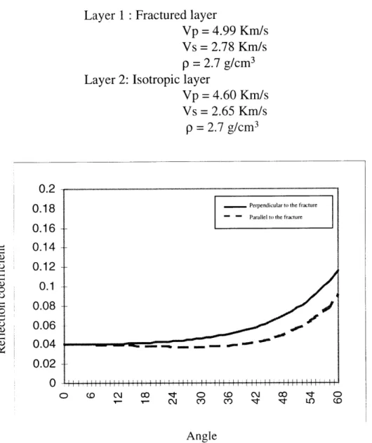
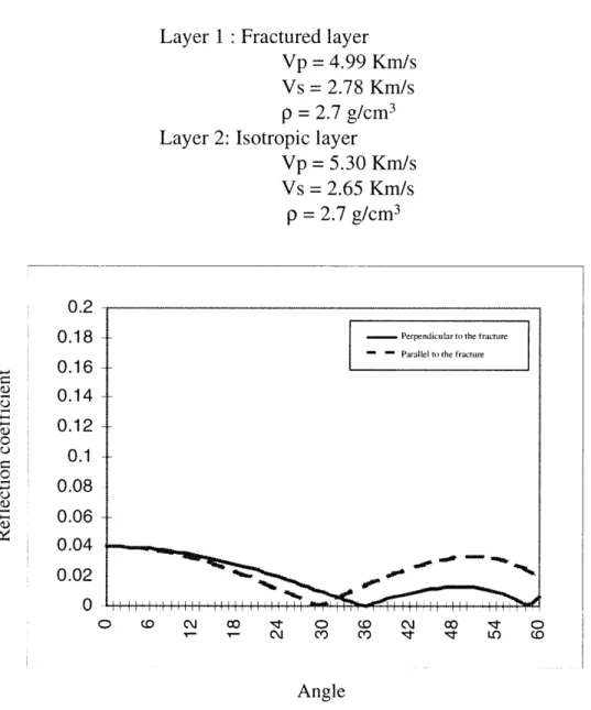
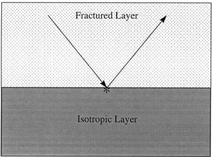
Some examples of calculated reflection coefficients for models of azimuthally anisotropic reservoirs illustrate this behavior. In Figures 1-3 and 1-4 we show the reflection coefficients for two models with a fractured layer over an isotropic layer with different velocity contrasts. Model 1 corresponds well to the model where the azimuthal P-wave AVO response is found in our field data further on in our study. We use Hudson's (1981) model to obtain the elastic constants for the fractured media. Then, we calculate the P-wave reflection coefficients solving the boundary conditions at the boundary of the two layers. The difference in P-wave AVO can be observed in the figures for lines parallel and perpendicular to the fractures. Thus, we can demonstrate that P-wave AVO is possibly a good indicator of azimuthal anisotropy. We expect to obtain similar results from our P-wave AVO analysis over the field data.

In a previous work, Ata and Michelena (1995) estimated the fracture orientation in a fracture reservoir using splitting measurements from the P-S converted data. The purpose of our study is to attempt to identify azimuthal P-wave AVO over the same fractured oil reservoir and compare it to previous independent results obtained using P-S converted waves to see if we can obtain similar results to identify fracture orientation.

1.2

Outline

In this chapter, we studied the azimuthal variation of AVO of field data in order to evaluate its applicability to the production geophysics environment.

In Chapter 2, we present a brief description of the area were the data were acquired, some details about the data acquisition, P and P-S converted wave data processing, AVO analysis results, and some discussion.

In Chapter 3, we present some results of the ray trace modeling using nearby well logs to build an earth model. We also compare the results obtained from the modeling to the field data.

Finally, Chapter 4 summarizes the results obtained in this work. Additionally, we describe some future related work.

Sources Receivers

Figure 1-1: Conceptual model. If the source-receiver azimuth is perpendicular to fracture orientation, at large angles of incidence, the reflection coefficients will be affected strongly by the hydrocarbons if there is sufficient gas in the oil.

Perpendicular

Figure 1-2: Effects of fractures in wave propagation. At large angles of incidence, the P-wave velocity is expected to be affected by the acoustic properties of the fluid filling the fractures when the wave propagation is perpendicular to the fractures, while it is less affected when the wave propagation is parallel to the fractures.

Layer 1 : Fractured layer

Vp =4.99 Km/s

Vs = 2.78 Km/s

p = 2.7 g/cm3

Layer 2: Isotropic layer

Vp =4.60 Km/s

Vs

2.65 Km/s

p

2.7

g/cm

0.2

0.18

Parallel to the fracture 0.16

0.14

0.12

0.1

0.08

0.06

0.04

-

0

Figure 1-3: Reflection coefficients vs. offset for a fractured medium over an isotropic media (Model 1).

Layer 1 : Fractured layer

Vp =4.99 Km/s

Vs = 2.78 Km/s

p

2.7 g/cm

Layer 2: Isotropic layer

Vp = 5.30 Km/s Vs = 2.65 Km/s

p

2.7 g/cm

0.2

0.16

0.14

0.08

0.06

0.04

0

Angle

Figure 1-4: Reflection coefficients vs. offset for a fractured medium over an isotropic media

(Model 2).

Perpendicular to the fracture

Parallel to the fracture

Chapter 2

Field Data: Maporal Field

2.1

Characteristic of the Field

The Maporal field is located in the north-central part of the Barinas-Apure Basin. Struc-turally, the Maporal field is a dome slightly extended in the NE direction. The geological setting is composed mainly of nearly flat-lying sediments. Two fault systems are present in the area. One runs southeast-northwest and the other northeast-southwest. A brief de-scription of the main formations present in the zone is shown in Figure 2-1. The target zone is the member 'O' of the 'Escandalosa' formation. It is a fractured limestone at a depth of approximately 3000 m (2.32 s). The fractures in the reservoir are filled with crude oil of approximately 28 API number. There is also evidence that some production comes from the 'P' and 'R' members of the stratigraphic section. These are composed mainly of sandstones; fractures also exist in these two members.

A number of wells exist in the field, which provide good background information on reservoir and fracture properties in the area, and which can be used for correlation studies. The well data includes sonic, dipole(shear), caliper, resistivity, gamma ray and other logs.

deter-mine the fractures that are more likely to be open or to be closed. Some maps of maximum horizontal stress and fracture strike in the field have been estimated using well logs (Fig-ures 2-2 and 2-3). The maximum horizontal stress runs southeast-northwest and different fracture systems have been identified. Based on the theory that open fractures tend to align along the direction of maximum regional stress, and consequently that perpendicular frac-tures may be closed, the fracture system of interest should be oriented southeast-northwest.

As we can see, the Maporal field is well suited for this study. The existence of fracturing is confirmed from in situ borehole observations, and we also have a preliminary estimate of orientation.

2.2

Data Acquisition

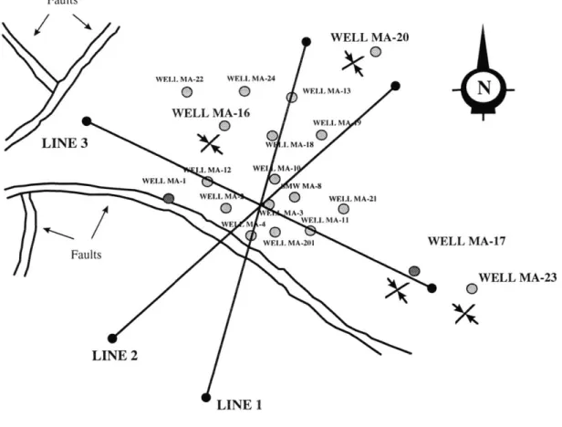
Three 10 Km three-component seismic lines were recorded over the area of interest along three different azimuths. The lines have a single intersection point. As was mentioned above, two systems of normal faults are present in the area. The azimuths of two lines (lines 1 and 3) were almost parallel to the fault systems, and the third line (line 2) almost bisected them and formed an angle of approximately 40 degrees with line 1. Figure 2-4 is an illustration of survey geometry with respect to the fault systems. A charge of one kilogram explosives at 10 m depth was used for the source. The source interval was set at 51 m and the geophone group interval at 17 m with a linear array between stations. The near offset trace was set at 17 m and the far offset extended to 3600 m, which satisfies the suggested minimum offset for an azimuthal AVO study (at least the same as the depth of the target zone). With this geometry we can expect a maximum incident angle of approximately 32 degrees for the target zone. A summary of the geometry of the survey and recording parameters is given in Table 2.1.

GEOMETRY

Number of traces 216

Total number of 3C receivers 648

Near offset trace 17 m ( 55ft)

Far offset trace 3672 m ( 12,000ft)

Number of elements per string 6

Separation of geophone elements 3.4 m

(l

Total geophone spread 10 Km

(

Total number of shotpoints per line 124

Shotpoint space interval 51 m

(

Charge depth 10 m

(

Charge size 1 Kg

(

Source offset 17 m

(

RECORDING

Total number of traces 648

Sample interval 2 ms

Low cut out

High cut 125 Hz

Notch filter out

Record length 6 s

Table 2.1: Survey parameters

2.3

Previous Studies

A study of S-wave birenfringence, or splitting, was previously conducted using this dataset by Ata and Michelena (1995). Due to the simple structure of the area, they used the asymptotic approximation (Tessmer and Behle, 1988;Tessmer et al., 1990) to calculate the

Common Conversion Point (CCP). Then, they applied rotation analysis to align observed data to the principal axes of symmetry and therefore to estimate the fracture orientation. They also made travel time studies (S1 and S2 modes) to estimate the fracture density.

As a result of this study a map showing the fracture orientation at the reservoir level was generated and is shown in Figure 2-5. Ata and Michelena (1995) concluded that lines 1 and 2 are nearly-perpendicular to fracture orientation, and line 3 is nearly-parallel to fracture orientation. We compare these results to our analysis.

2.4

AVO Study

The first goal of our work is to perform AVO analysis of the P-wave data. Specifically, we focuse on the intersection point of the three seismic lines. At this point, all lines should be looking at the same point in the subsurface and we will compare the differences in the azimuthal response.

2.4.1 P-wave Data

2.4.1.1 Data Processing

The basic objective of the data processing for AVO analysis is to preserve relative amplitude for all offsets at all times for any CDP gather. Additionally, relative amplitudes among all depth points need to be preserved. In the case of stacked data, the process of CDP stacking cancels many types of noise. However, in the prestack domain the processor cannot count on this tool. Many processing schemes for AVO analysis have been presented in the literature and some of them are presented in Appendix B.

The same data processing sequence was applied to all lines using a basic but robust scheme in order to conserve the reflectivity variation with offset. A subset of the data was extracted from the original one to consider the area of the reservoir near the intersection point. The

number of shots selected guaranteed maximum fold over the cross point (36 traces). Special emphasis in the processing was made around the cross point of the lines, at approximately CDP 224 of the reduced dataset. The processing sequence applied to all lines was:

1. Spherical divergence correction:

The data was received with spherical divergence applied. Therefore, no correction was necessary at this point.

2. Coherent noise suppression:

F-k filtering was applied to the data in order to suppress coherent noise such as ground roll and guided waves.

3. Velocity analysis and statics iterations:

Several iterations of semblance velocity analysis and statics corrections were applied to obtain a better quality in the NMO-corrected CDP gathers. The semblance velocity analysis at the interception point for the three lines is similar and is presented in Figure 2-6. The maximum power autostatics method was applied to all lines in order to maximize the CDP stack power.

4. NMO correction:

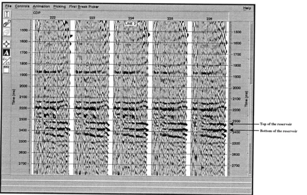
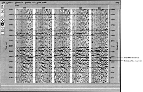
Standard NMO correction was applied to all CDPs. It is known that the NMO stretch decreases frequency at far offsets, which affects the amplitudes. However, this distortion is significant at shallow depths and at a large offset. The target zone in our study is relatively deep and the stretch problem does not significantly affect the results. NMO-corrected gathers around the intersection point for the three lines are presented in Figures 2-7, 2-8 and 2-9.

5. AVO analysis:

AVO analysis was made over the three lines. A detailed description of the procedures and results of the AVO analysis are presented in the next section.

Finally, we stack the three lines. The results obtained for the three lines are presented in Figures 2-10, 2-11 and 2-12. In these figures we can corroborate the simple structure of the area described above.

In addition, we made a spectral analysis over the data; the center frequency was found to be around 25 Hz.

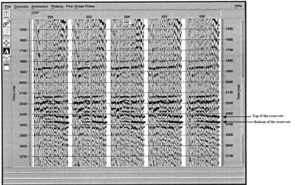
As it is known, deconvolution is a process that improves the temporal resolution by com-pressing the seismic wavelet. It is often used to isolate seismic events, which is important for AVO analysis. We point out that we did not use deconvolution in order to conserve amplitude information. However, the results obtained from our data processing correspond well to the results obtained from our ray tracing modeling, which is shown in Chapter 3. Finally, it is important to note the consistency of the processing among all lines, which is supported by the good tie between the three lines (see Figure 2-13). The top of the fractured reservoir is located at 2320 ms and the base at 2370 ms. A higher frequency can be observed at the reservoir level for the line parallel to fracture orientation (line 3). However, these results are consistent with the ones obtained by Lynn et al. (1996), where the frequency content is related to source-receiver azimuth relative to fracture strike.

2.4.1.2 AVO Analysis

AVO analysis was made for each line and the AVO gradient and intercept were obtained. For AVO analysis, the PROMAX module AVO Attribute Stack was used. AVO Attribute Stack is a tool used to analyze the relative amplitudes within a pre-stack, NMO-corrected CDP gather. A common problem with AVO analysis is residual NMO on the CDP gathers resulting from imperfect velocity specification. In order to compensate for this problem, this tool allows one to select the amplitudes within polarity gates (see Figure 2-14), reducing the requirement for exact NMO application. Polarity gates are determined for partial stack of the data in the CDP gather. Contiguous stack amplitudes with a common polarity define a

polarity gate. The data within each polarity gate is condensed, selecting either the maximum or the average amplitude on each trace within the gate. We used the maximum option in our analysis. A robust least squares line is fitted to the amplitudes of each trace, and the AVO intercept and AVO gradient are computed from the fit to the data (see Figure 2-15).

An AVO anomaly with a large positive gradient was found near the base of the Escandalosa formation in lines 1 and 2, perpendicular to fracture orientation (see Figures 2-16 and 2-17). This AVO anomaly is not present in line 3, parallel to fracture orientation (see Figure 2-18). The AVO gradient versus AVO intercept graph for CDP gathers of each line around the cross point shows the high positive gradients for the lines perpendicular to the fracture, while they are smaller for the line parallel to the fracture (see Figure 2-19 ).

The AVO intercept for the bottom of the reservoir is very small for all lines (see Figures 2-20, 2-21 and 2-22). Theoretically, it should be the same for all lines no matter the source-receiver azimuth relative to fracture strike. However, some small differences were observed that could be caused by some noise in the data.

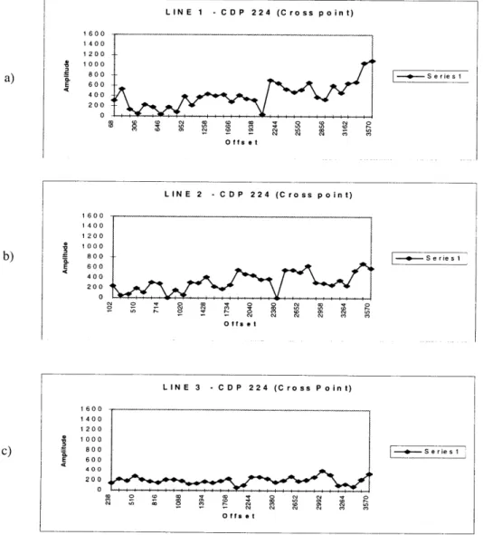
A detailed example of the behavior of the amplitudes for the cross point CDP gather for each line is shown in Figures 2-23a, 2-23b and 2-23c. These figures also show that an increase of the amplitude with the offset is larger for the lines perpendicular to the orientation of the fractures (lines 1 and 2) than for the line parallel to the orientation of the fractures (line 3).

2.4.1.3 Discussion

To start the discussion of the obtained AVO response, we present two of the five rules em-pirically established by Koefoed (1955) about the effects of Poisson's ratio on the reflection coefficients of plane waves:

1. "When the underlying medium has the greater longitudinal P-wave velocity and the other relevant properties of the two strata are equal to each other, an increase of

Poisson's ratio for the underlying medium causes an increase of the reflection coeffi-cient at the larger angles of incidence." Shuey (1985) points out that the qualifications concerning the medium properties are not necessary for this and the next rule. 2. "When, in the above case, Poisson's ratio for the incident medium is increased, the

reflection coefficient at the larger angles of incidence is thereby decreased."

The azimuthal difference in AVO gradients can be explained by a low Vp/Vs ratio for the lines perpendicular to the fracture due the inluence of the fluid filling the fractures, resulting in a large positive contrast in Poisson's ratio with the lower layer, and a very positive AVO gradient anomaly. For the line parallel to the fracture, the Vp/Vs ratio is less affected by the fluid filling the fractures and is greater than the previous case. This corresponds to rule number 2 and therefore the AVO anomaly is not present.

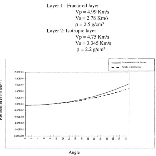
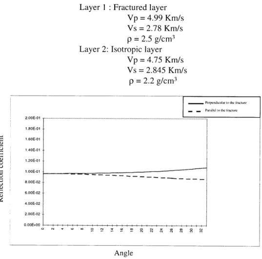
Until this point, we have been analyzing the results with the isotropic idea in mind. As we mentioned before, it has been shown that the reflection coefficient response depends on the source-receiver azimuth related to fracture orientation. However, there are only a few studies (e.g., Riiger, 1996) that relate AVO attributes to crack parameters. What seems to be clear is that the P-wave AVO gradient is affected by fracture-induced azimuthal anisotropy. In order to analyze our results using azimuthal differences in the reflection coefficients due to source-receiver azimuths, we calculate some reflection coefficients curves in two azimuths (one parallel and the other perpendicular to fracture orientation), and compare them to our results. We use information about the velocities (V and V) and densities at the bottom of the reservoir from nearby well logs to build our two-layer model. Layer 1 is a fractured layer and layer 2 is an isotropic one (see Figure 2-24). We use Hudson's (1981) theory to estimate the elastic constants, using a fracture density of 0.1, and a bulk modulus for fluid filling the fractures that approximates an oil of 28 API (Batzle and Wang, 1992), as the one we have in the reservoir. Thomsen's (1986) anisotropic coefficients for the fractured layer are shown in Table 2.2. Different results were obtained changing only 17, and consequently the relation of the V,/V ratio between the two layers (see Figures 2-25, 2-26 and 2-27). Model 1 corresponds very well to the results obtained from our data where the AVO gradient is

bigger for the lines perpendicular to fractures (lines 1 and 2) than for the line parallel to the fractures (line 3).

e 0.3035 Y -0.1

6 -0.0062

Table 2.2: Thomsen's anisotropic coefficients for the fractured layer in models 1, 2 and 3

No azimuthal AVO anomaly is apparently observed at the top of the fractured reservoir. We calculate the reflection coefficient for this interface (see Figure 2-28), using data from well logs (see Figure 2-29). Thomsen's anisotropic coefficient for the fractured layer in this model, are presented in Table 2.3. We can observe a difference between the two lines (perpendicular and parallel to fractures), however it is smaller than for the bottom of the reservoir, and could also be reduced for some tuning effects. We do not get the anomaly we expect from the top of the reservoir from our field data, but we show in Chapter 3 that this behavior can be reproduced by synthetic seismograms.

E 0.28 -Y -0.09

6 -0.003

Escandalosa formation

(reservoir)

~/;

R sand

Faults

WELL MA-20

)(

0

0 0 WELL MA-16 G MA-21 Faults LINE 2 LINE 1

Figure 2-2: Maximum horizontal stress estimated from borehole ellipticity. Arrows indicate the estimated direction of the maximum horizontal stress field.

W

N

WELL MA-17

WELL MA-23 0

Faults

WELL MA-22 WELL MA-24

0 N

/

4

Faults

180

WELL MA-20

WELL MA-22 WELL MA-24

590

(D WELL MA-13

WELL MA-16

LINE 3

LINEL3NE

W2..L MA-18 AL MA-12 WEI MA-I(

WELL MA-I

W MA-8

WELL MA-2 WELL MA-21

A-3

(

E M -4 WLL MA-11

WELL MA-201

Faults WELL MA-17

WELL MA-23

118*

LINE 2

LINE 1

LINE 3

LINE 2

LINE 1 tu uf t e

Figure 2-5: Map view of fracture orientation at reservoir level, obtained from rotation analysis of the three lines (Ata and Michelena, 1995). The orientation is in general quasi-parallel to line 3 and quasi-perpendicular to lines 1 and 2.

Figure 2-6: Velocities at the cross point from semblance velocity analysis. Semblance Analysis 0 In 0 -- LINE1I 8Q--- LNE 2 0* -*- LNE 3 0 i i I ! l I I I i I I

i

~

1113- 11- -1 Tipp 4)f the reserviir

pa- Bottom (if the reservoir

MWf oi. MI/*llu Hl fif

-Top of the reservoir

Fottom of the reservoir

Top of the reervoir - ottom of the reservoir

rnp or the rervoir

- Bottom of the reservoir

Top r the reservoir

BFttom of the reservoir

Tip of the reservoir

Bottom of the reservoir

Figure 2-12: Stacked section - line 3.

y -Top of the reservoir

Figure 2-13: The consistency of the processing among all three lines is supported by the good tie between all of them at the cross point.

Polarity Window

Stack

Trace 400

Input Gather Offset

-I

~(.~

/

,:

~'

Polarity

Gate

... ... $*ne moo @?se a go@aIeeoxrem el as 66 s$ ls . ..

's 006 Oe

Figure 2-14: Polarity gate for 'AVG Attributes Stack' Analysis.

Amplitudes

Sin

2

I- AVO intercept, reflection coefficient Rp at normal incidence

B- AVO gradient, slope

cross point

Top of the reservoir F 1ttim 2 theA rgrvor

cross point

- Tipp of the reservoir

-- 1hottom of the reervoir

cross point

Top of the reservoir Bottom of the reservoir

AVO Intercept vs. AVO Gradient 1200-0 1200-0 809 S

ii

Figure 2-19: AVO intercept vs. AVO gradient for lines 1, 2 and 3.

* LINE 1 * LINE 2

A LINE 3

cross point

Top a th repervoir

Figure 2f 20e A n e re ereo

cross point

Top ofthe rv~rvo.ir

Bottiom (fthe resrvoir

cross point

Figure 2-22: AVO intercept for line 3 (parallel to fracture orientation).

TNo o~f the reservir

LINE 1 - CDP 224 (Cross point) 1600 1400 1200 1000 a800 -Series I E 600 400 200 0 -o ffs et

LINE 2 - CDP 224 (Cross point)

1600 1400 1200 1000 b) 8 0 Seres 1600 400 200 0 L1 i + _ __ NO n 0 0 N1 D ' 0 -8i 1000 q 00 U M w r C) c to MSeries1 -0 1. ff t

LINE 3 - CDP 224 (Cross Point) 1 600 1 400 1 200 1000 C) 800 -.- S er ie s 1 E 600 400 200 0 4 0 D O 't 4 OD N Nl -T 0 t 0 t

Figure 2-23: Amplitudes vs. offset for the CDP at the cross point. (a) Line 1, perpendicular to fracture orientation. (b) Line 2, perpendicular to fracture orientation. (c) Line 3, parallel to fracture orientation.

I

I

I

Layer 1 Fractured layer Vp = 4.99 Km/s Vs = 2.78 Km/s

p = 2.5 g/cm3

Layer 2: Isotropic layer Vp = 4.75 Km/s Vs = 3.345 Km/s

p = 2.2 g/cm3

Perpendicular to tie Iracture Parallel to the Iracture

1.80E-01 I. 1.60E-01 1.40E-01 1.20E-01 1.00E-01--<U 8.00E-02 6.00E-02--4-00E-02 2.OOE-02 0.00E+00 oG o a e e o o nli ' W Go o nli Angle

Layer I : Fractured layer Vp = 4.99 Km/s

Vs = 2.78 Km/s

p = 2.5 g/cm3

Layer 2: Isotropic layer Vp = 4.75 Km/s

Vs = 2.845 Km/s

p = 2.2 g/cm3

Perpendicular to the Iracture Parallel to the fracture

-.. ----. ... .. .... .. .. .. ... ... ... ... ... ... ... ... .... .. .. .. ... .. . ... ... .. ... ... .. ... ... .

-- -- - -

-Angle

Figure 2-26: Reflection coefficients vs. angle at the bottom of the reservoir (Model 2).

2.00E-01 1.80E-01 1.60E-01 1.40E-01 1.20E-01 1.OOE-01 8.00E-02 6.00E-02 4.00E-02 2.00E02 -0.00E+00 , , , , 0 C\1 2 ON CN\j C-T\j , w C\j Co Co0 c\J

Layer I : Fractured layer Vp = 4.99 Km/s Vs = 2.78 Km/s

p

2.5

g/cm

Layer 2: Isotropic layer

Vp =4.75 Km/s

Vs = 2.345 Km/s

p = 2.2 g/cm3

PerpendicuIar to the Iracture Parallel to the -racture 2.00E-01 1.80E-01 1.60E-01 1.40E-01 1.20E-01 1.00E-01 8.00E-02 0) 6.000-02 . 2.00E-02 .00E+00 Angle

Fractured L

Layer 1 : Isotropic layer Vp = 3.345 Km/s Vs= 1.580 Km/s

p = 2.4 g/cm3

Layer 2: Fractured layer Vp = 4.99 Km/s

Vs = 2.78 Km/s

p = 2.5 g/cm3

Perpendicular to the Iracture

Parallel to the I racture

2.00E-0 .--... 1.80E-01 1.60E-01 1.40E-01 o 1.20E-01 1.00E-01 S.00E-02 6.00E-02 4.00E-02 2.00E-02 0 00E+00 ,. , , N C N 10 Angle

Chapter 3

Modeling

AVO analysis shows an anomaly near the bottom of the Escandalosa formation (reservoir). In order to interpret the results and confirm our conclusions from AVO analysis, we built a realistic earth model at the cross point of the three lines using well log data. Synthetic seismograms were computed using ray tracing to simulate the field data. The results show that the P-wave AVO can reproduce the type of anomaly observed in the field data.

3.1

Well Logs

The data used in this study correspond to a producting area. Consequently, many wells are present in the area, most of them with different types of logs. Three different wells were studied to build an earth model that is realistic and that reproduce seismic properties of the relevant formations. The wells were well MA-1, well MA-17 and well TOR-2X (see Figure 3-1). As was mentioned previously, the geology of the area is very simple, and all main formations are present across it. This allows a good correlation between wells in the interpretation process.

P-wave velocities (see Figure 3-2). Unfortunaly, well MA-17 does not extend to the bottom of the reservoir where the AVO anomaly was found in the field data. Well MA-i does have a resistivity log that extends to the basement. P-wave velocities were estimated from the resitivity log using Faust's (1953) approximation. Faust found an empirical formula for velocity in terms of depth of burial z and formation resistivity R

Vp = 900(zR)1/6 (3.1)

Vp being in m/s, z in n, and R in Q.m. Then, densities were estimated using Gardner's

rule. Gardner et al. (1974) graphed velocity against density and found that the major sedimentary lithologies defined a relatively narrow swath across the graph. They determined an empirical equation relating velocity and density, often called Gardner's rule:

p = aV1/4 (3.2) where density p is in g/cm3, a = 0.31 when velocity is in m/s and a = 0.23 when V is in ft/s. Estimated density and P-wave velocity logs are shown in Figure 3-3. Finally, S-wave velocities were obtained from P-wave velocities using different ratios V,/V, between 1.5 and 2.0. Well TOR-2X does not belong to the Maporal field, but it is located in a field nearby in the Barinas basin. The geology is very similar to all main formations at the Maporal field also present in this area. Well TOR-2X has a sonic log (see Figure 3-4) that extends to the basement, and was used to calibrate the velocities obtained from the resistivity log in well MA-1. Velocities for each formation were compared in order to validate the approximated ones obtained in well MA-1.

3.2

The Model

A flat layer structure was assumed for the earth model of the Maporal field. This is a realistic model of the real geological structure. Additionally, our study was concentrated at the cross point of the three lines, and no other structural details were needed. An eight layer model was built (see Figure 3-5) using the well logs presented in the previous section. The elastic properties of formations Gobernador, Burguita and Quevedo were averaged and

modeled as a single layer. The '0' member of the Escandalosa formation (reservoir), has the primary fracture concentration, and was modeled as an anisotropic layer due to vertical fractures, as is evidenced from the televiewer logs of nearby wells. There is also evidence from the televiewer logs of the presence of fractures in the members 'P' and 'R' of the same Escandalosa formation. Therefore, these two members were also modeled as vertical fractured layers, even though the fracture density modeled was smaller than for the '0' member. All other layers were modeled as isotropic layers.

We computed the elastic constants for the anisotropic layers using Hudson's (1981) theory for the properties of the fractured layer. Different experiments were made changing the fluid content in the fractures to analyze the effect of fluid in the P-wave AVO seismic response. In our study we label as light oil those with a high API number, which have higher gas content, and heavy oils, which have low API. The API number is about 100 for light condensates and nearly five for very heavy oils. The fractures in the reservoir are filled with crude oil of approximately 28 API, which we call medium oil. In our experiments we used the following as fluids: gas, light oil, medium oil, heavy oil and water. To calculate the elastic constants for the different fluids filling the fractures in the media, we use an approximation of the bulk modulus for different API numbers (Batzle and Wang, 1992). A detailed table including computational parameters and model material properties, for the fracture layers ('0' member and 'P' and 'R' sandstones), used for all cases (gas, light oil, medium oil, heavy oil and water) are given in Appendix C.

3.3

Synthetic Data

3.3.1 Synthetic Seismograms

We computed synthetic seismograms for the eight layer model, using 3D paraxial ray trac-ing (Gibson et al., 1991). _{Two sets of seismograms were calculated for each case (gas,} light oil, medium oil, heavy oil and water), one perpendicular to fracture orientation and

the other parallel to it. Seismograms were calculated in shot gathers, using 25 receivers that guarantee the same minimum (17 m) and maximum offset (3672 m) as the field data. Because we have a horizontal layer model, this geometry is equivalent to a CDP gather at the cross point. The wavelet was extracted from the field data in order to use a similar one in the modeling process. An explosive type of source was used and the wavelet correspond to the function symetrical - eccponential * cosine. A center frequency of 25 Hz was used to calculate the seismograms, as was found in the field data. Geometrical spreading was neglected in the calculations, so no additional processing was required to eliminate this effect. We processed each gather and obtained the NMO corrected gathers. The synthetic seismograms for one model (parallel to fractures filled with medium oil) were compared to the field data by copying the trace obtained by stacking the synthetic CDP gather to create a small section. The good correlation of the seimic events between the modeled data and the field data is shown in Figure 3-6. Some mismatches are observed between the first seismic event and the top of the reservoir because the formations Gobernador, Burguita and Quevedo were averaged as a single layer.

3.3.2

AVO Analysis

AVO analysis was made for each gather using the same AVO Attribute Stack PROMAX tool, that was previously used with the field data. The AVO gradient was obtained for each gather. Figures 3-7 and 3-8 show the AVO gradient for the wave propagation perpendicular and parallel to the fractures filled with gas, Figures 3-9 and 3-10 show the case of fractures filled with light oil, Figures 3-11 and 3-12 show the case of fractures filled with medium oil and Figures 3-13 and 3-14 show the case of fractures filled heavy oil. Finally, Figures 3-15 and 3-16 show the results of the AVO gradient obtained for the case of water filling the fractures. These figures show that the AVO gradient at the bottom of the reservoir is greater for the lines perpendicular to the fractures compared to the lines parallel to them. It can also be observed that this difference is greater when the gas content in the fluid filling the fractures is also larger.

Detailed graphs of the P-wave amplitudes vs. offset for the bottom of the reservoir were obtained from the synthetic seismograms for all of the cases (Figure 3-17). The percentage differences in the AVO gradient, between the lines perpendicular and parallel to fractures for all cases, are presented in Figure 3-18. The difference in AVO gradient is greater as the gas content in the fluid increases.

3.4

Discussion

We compare the P-wave AVO analysis over the synthetic seismograms around the bottom of the reservoir to the results obtained from the field data (see Figures 3-17 and 3-19). Even the absolute values are not the same, they exhibit similar trend near the bottom of the reservoir, where the AVO gradient is bigger for the lines perpendicular to fracture orientation than for the line that is parallel to it. This behavior is obtained using an oil to fill the fractures with a similar API to the one produced in the field.

Although we know that the main concentration of fractures is at the top of the reservoir ('0' member), the AVO anomaly is observed around the seismic event that has been interpreted as the bottom of the reservoir. However, because the '0' member and the 'S' shale are very thin layers, and also the 'P' and 'R' sandstones conform an small one, some tuning effects can change the waveforms and the amplitude content (see Figure 3-20). The reflections associated with the 'O'member start in the seismic time section at the "depth" (time) of the '0' member, but extend below it, being superposed with other events from 'P' and 'R' members (top and base). Likewise, the reflections from the top and the bottom of the '0' member is combined together in the seismic section. Therefore, one of the major goals of the ray tracing modeling was to check if the response of the 'combination' of reflections from the different interfaces reproduce the observed pattern of AVO variations of the field data. The results obtained from the synthetic data comfirm the same results obtained from the field data. We also did some ray calculations using a similar model, but with fractures only in the '0' member, and they yield to fairly similar results. Some deconvolution could

help to improve the vertical resolution and identify individual reflections, but we decided not to do so to try to better preserve accurate amplitudes.

We showed, with field and synthetic data, that the P-wave AVO response depends on the orientation of the shot line with respect to the fractures. These results demostrate that P-wave AVO may be useful to detect azimuthal anisotropy and potential fracture orientation.

No AVO gradient anomaly is obtained at the top of the reservoir from the synthetic data. This confirm the results obtained from the field data.

WELL TOR-2X Faults 0 0 Faults LINE 2 LINE 1

Figure 3-1: Well logs used to build an earth model at the cross point of the three lines.

WELL MA-17

WELL MA-17 <Vp> _m/r/ <Vs> . - GOBERNAI)OR - IA MOITA - ESCANIDALOSA - PSANI)STONE

Figure 3-2: P-wave and S-wave velocities obtained from a dipole sonic log in well MA-17.

62 Depth 944MI 95INI 96MI 971M) 99Mi 1011) 1021N) 1051MI 105(9) 1061M) 11171NI 10MINI

IWELL MA- 1]

<DTI -Vers:I> <GARDNER> Depth Vs/ft g/cc 94410N ... 9501 - .. . -CO ERNADOR 964N) 974M) 9800) 10414NI 102M- ' -4A MORITA 103(NI -RSCANDALOSA 104Mw - - - -1'SANDSTONE 11151N1 14164NI -S SHALE -M - -- - -- -AGUARDIENTE 1084NI -- .. - -RiASEMENT

Figure 3-3: Density and sonic logs obtained from a resistivity log in well MA-1, using Gardner's and Faust's approximations.

WELL TOR-2X L i Lr ---DTC - Vers: 9s/ft Time 150 60 1750 h1800 -- -- PAGUEY -1850) -19(H) -1950 -2000 -2050 - - - - GOBERNADOR -2150 -22(H)

- -- .- ESCANDALOSA ('O' member)

--- -- PSANDSTONE

-2250

_ _SSHALE

-AGUARDIENTE -2300 BASEMENT

Figure 3-4: Sonic log in well TOR-2X.

64 Feet 8400-86001 8800 9000 k 92() -94(m) -96(M 9800 -10000 -10201 -10400 -10600 - 10800 -IW 11200 -11400 11600 .

p = 2.3g/cm3 Vp = 3157m/s Vs = 1579n/s p = 2.4g/cn I Vp = 3726n/s Vs = 2053in/s p = 2.4g/cm 3 Vp = 3345ims Vs = 1580n/s p = 2.5g/cm 3 Vp = 3513m/s Vs = 1887m/s 3340m 3640m 3670m 3691 m p = 2.7g/cm3 Vp = 4994m/s Vs = 2784m/s

R sand

Aguardiente

...

Figure 3-6: Comparison of stacked synthetic seismogram to field data. The synthetic seis-mogram (middle) corresponds to the propagation parallel to fractures filled with medium oil. Some mismatches are observed between the first event and the top of the reservoir because the formations Gobernador, Burguita and Quevedo were averaged as a single layer.

- Top of the reservoir Bottom of the reservoir

Figure 3-7:

Synthetic

- Top of the reservoir

Bottom of the reservoir

Figure 3-8: Synthetic AVO gradient for a line parallel to fracture orientation. Fractures filled with gas.

220Top of the reservoir

Bottom of the reservoir

Figure 3-9: Synthetic AVO gradient for a line perpendicular to fracture orientation. Frac-tures filled with light oil.

.... ... .. . . op of the reservoir Bottom of the reservoir

Figure 3-10: Synthetic AVO gradient for a line parallel to fracture orientation. Fractures filled with light oil.

Figure 3-11: Synthetic AVO gradient for a line perpendicular to fracture orientation. Frac-tures filled with medium oil.

.. .Top of the reservoir Bottom of the reservoir

Figure 3-12: Synthetic AVO gradient for a line parallel to fracture orientation. Fractures filled with medium oil.

Top of the reservoir

Bottom of the reservoir

Figure 3-13: Synthetic AVO gradient for a line perpendicular to fracture orientation. Frac-tures filled with heavy oil.

.. Top of the reservoir

Bottom of the reservoir

Figure 3-14: Synthetic AVO gradient for a line parallel to fracture orientation. Fractures filled with heavy oil.

--- .- . - Top of the reservoir ottom of the reservoir

Figure 3-15: Synthetic AVO gradient for a line perpendicular to fracture orientation. Frac-tures filled with water.

... op of the reservoir Bottom of' the reservoir

Figure 3-16: Synthetic AVO gradient for a line parallel to fracture orientation. Fractures filled with water.

Gas 3.506 02 -.-. ---.. ..--- - -.----.. ----. ---... 3 -02 .WE !2.50602 1 50602 3.505 02 ---. --- .. - -. .... -.. . ... . 2-50602

2,00602

Figure 3-17: P-waves amplitudes vs. offset for the bottom of the reservoir. Fractures filled with (a) gas, (b) light oil, (c) medium oil, (d) heavy oil, and (e) water.

10.29

7.37

5.52

Gas Light Oil Medium Oil Heavy Oil Water

Fluid Filling fractures

Figure 3-18: Percentage differences in AVO gradients. Perpendicular - Parallel to fracture orientation

Amplitude vs. Offset at the crosspoint Field Data -- -q- 0o <0 CM< cj o 00 (0 0 0 ( o N - o 0o a o 0 -- N - c\j c\J (0 (0 Co c ) N 0 0) (o 0o 0 c\1 Uo N 0) 0 c\j Ln Offset --- LINE1 --- LINE 2 LINE 3

Figure 3-19: Comparison of P-waves amplitudes vs. offset at the bottom of the reservoir

-Field Data 1400 1200 1000 800 600 400 200 0 -200

Receiver

Figure 3-20: Tuning effect. The reflection from the top and interfere, and result in a composed signal (b). Waveshapes and original signal.

the base of the layers (a) amplitudes differ from the

Tuning

Chapter 4

Discussion and Conclusions

From the azimuthal dependent AVO analysis at the crosspoint of three 2D seismic lines, over a fractured reservoir, the following conclusions can be made:

1. In the presence of fracture induced azimuthal anisotropy, the P-wave AVO response may depend upon azimuth.

2. The results obtained using azimuthal-dependent P-wave AVO analysis are consistent with the results obtained in a previous study with the same field data using P-S converted waves.

3. The modeling results, using information from nearby wells, show the same trend as the field data.

4. Azimuthal P-wave AVO analysis can aid in detecting azimuthal anisotropy and frac-ture orientation.

One limitation in this work was that 2D data allowed the analysis of only one surface location (intersection point of the three seismic lines). There is a 3D survey over the same area, and in the future we will do azimuth-dependent AVO analysis using this dataset to confirm the results obtained in the present work.

Appendix A

AVO Theory

(From Castagna, 1993a)

The variation of reflection and transmission coefficients with the incident angle (and corre-sponding increasing offset) is referred to as offset-dependent-reflectivity and is the funda-mental basis for amplitude-versus-offset (AVO) analysis.

In exploration geophysics, we rarely deal with simple isolated interfaces. Nevertheless, it is easier to understand offset-dependent reflectivity as the partitioning of energy at just an interface. We must be careful, however, to remember that most reflections we see are a superposition of events from a series of layers, and will have a more complex AVO behavior than will be shown here.

Consider two semi-infinite isotropic homogeneous elastic media in contact at a plane inter-face. Further, consider an incident compressional plane wave impiping upon this interinter-face.

The plane-wave assumption is valid at source-to-receiver distances, which are much longer than the wavelength of the incident wave and are generally acceptable for precritical reflec-tion data at explorareflec-tion depths and frequencies. As shown in Figure A-1, reflecreflec-tion at an interface involves energy partition from an incident P-wave to (1) a reflected P-wave, (2) a transmitted P-wave, (3) a reflected S-wave, and (4) a transmitted S-wave. The angles for