HAL Id: inserm-00133006
https://www.hal.inserm.fr/inserm-00133006
Submitted on 26 Feb 2007HAL is a multi-disciplinary open access archive for the deposit and dissemination of sci-entific research documents, whether they are pub-lished or not. The documents may come from
L’archive ouverte pluridisciplinaire HAL, est destinée au dépôt et à la diffusion de documents scientifiques de niveau recherche, publiés ou non, émanant des établissements d’enseignement et de
Choice between semi-parametric estimators of Markov
and non-Markov multi-state models from coarsened
observations
Daniel Commenges, Pierre Joly, Anne Gégout-Petit, Benoit Liquet
To cite this version:
Daniel Commenges, Pierre Joly, Anne Gégout-Petit, Benoit Liquet. Choice between semi-parametric estimators of Markov and non-Markov multi-state models from coarsened observations: Choice be-tween semi-parametric estimators of Markov and non-Markov multi-state models. Scandinavian Jour-nal of Statistics, Wiley, 2007, 34, pp.33-52. �10.1111/j.1467-9469.2006.00536.x�. �inserm-00133006�
Choice between semi-parametric estimators of
Markov and non-Markov multi-state models
from coarsened observations
Daniel Commenges
1,2, Pierre Joly
1,2, Anne G´egout-Petit
2, Benoit Liquet
31 INSERM, U 875, Bordeaux, F33076, France
2 Universit´e Victor Segalen Bordeaux 2, Bordeaux, F33076, France 3 Universit´e de Grenoble, F33000, Grenoble
Running title: Choice between semi-parametric estimators ABSTRACT. We consider models based on multivariate count-ing processes, includcount-ing multi-state models. These models are spec-ified semi-parametrically by a set of functions and real parameters. We consider inference for these models based on coarsened obser-vations, focusing on families of smooth estimators such as pro-duced by penalized likelihood. An important issue is the choice of model structure, for instance the choice between a Markov and some non-Markov models. We define in a general context the ex-pected Kullback-Leibler criterion and we show that the likelihood based cross-validation (LCV ) is a nearly unbiased estimator of it. We give a general form of an approximate of the leave-one-out
LCV . The approach is studied in simulation and illustrated by
es-timating Markov and two semi-Markov illness-death models with application on dementia using data of a large cohort study.
Key Words: counting processes, cross-validation, dementia, interval-censoring,
Kullback-Leibler loss, Markov models, multi-state models, penalized likeli-hood, semi-Markov models.
HAL author manuscript inserm-00133006, version 1
HAL author manuscript
1
Introduction
Multi-state models, and more generally models based on multivariate count-ing processes, are well adapted for modelcount-ing complex event histories (An-dersen et al., 1993; Hougaard, 2000). Assumptions have to be made about the law of the processes involved. In particular the Markov assumption has been made in many applications (Aalen & Johansen, 1978; Joly et al., 2002) while semi-Markov models have been considered in other applications (Joly & Commenges, 1999). Subject-matter knowledge can be a guide for mak-ing these assumptions (for instance risk of AIDS essentially depends on time since infection, leading Joly & Commenges (1999) to choose a semi-Markov model); however in many cases the choice is not obvious. Other assumptions have to be made relative to the influence of explanatory variables: multi-plicative or additive structures for instance may be considered. The problem is generally not to assert whether the “true” model is Markov or has a mul-tiplicative structure but to choose the best model relative to the data at hand.
The semi-parametric approaches offer the greatest flexibility. Aalen (1978) has studied non-parametric inference for counting processes. If we wish to estimate smooth intensities we have to consider families of estimators such as kernel estimators (Ramlau-Hansen, 1983), sieve-estimators (Kooperberg & Clarkson, 1997) or penalized likelihood estimators (Good & Gaskin, 1971; O’Sullivan, 1988; Joly et al., 2002). These families are indexed by a param-eter that we may call “smoothing coefficient”. A practical way for choosing the smoothing coefficient is by optimizing a cross-validation criterion. In particular likelihood cross-validation (LCV ) has been shown to have good properties in simulation (Liquet, Sakarovitch & Commenges, 2003; Liquet & Commenges, 2004) while it has been shown that in some cases it could be con-sidered as a proxy for the expected Kullback-Leibler loss and had the optimal property of being asymptotically as efficient as this theoretical criterion (Hall, 1987; van der Laan, Dudoit & Keles, 2004). Liquet, Saracco & Commenges (2006) argued that LCV could be used not only for choosing the smoothing coefficient but also for choosing between different semi-parametric models, such as stratified and non-stratified proportional hazard survival model.
Additional complexity comes from the fact that the model must be es-timated from incomplete data. Coarsening mechanisms have been studied in a general context by Gill, van der Laan & Robins (1997). Commenges & G´egout-Petit (2005) have studied a general time-coarsening model for
cesses which they called GCMP; we will use this coarsening process under the name TCMP for “time-coarsening model for processes”; in effect it is not completely general because it assumes that there are times where the process is exactly observed; this is most often the case for counting processes but not for more general processes. Even for counting processes the TCMP does not include the filtering process of Andersen et al. (1993) in a natural way. Writing the likelihood for observations of multi-state models through the TCMP has been done by Commenges & G´egout-Petit (2006).
The aim of this paper is to advocate the use of the expected Kullback-Leibler risk, EKL, based on the observation, for the choice between semi-parametric estimators for coarsened observations. We also advocate the use of LCV as an estimator of EKL. Thus LCV can be used in particular for choosing between estimators of Markov and non-Markov multi-state models or between multiplicative and additive models in the presence of generally coarsened observations. It is worth noting that the LCV choice fits well with using families of smooth estimators, such as produced by penalized likelihood, because non smooth estimators are strongly rejected by this criterion.
In section 2 we recall the description of multi-state models as multivariate counting processes and suggest possible Markov and non-Markov structures for the illness-death model. In section 3 we recall the construction of the likelihood ratio for counting processes and its extension to penalized like-lihood and we unify the problem of choice of smoothing coefficients and model structure. In section 4 we tackle the problem of likelihood ratio and penalized likelihood in the TCMP framework. In section 5 we define the ex-pected Kullback-Leibler loss as a general criterion for choosing an estimator in a family of estimators based on generally coarsened observations; we also study the case where there are observed explanatory variables. In section 6 it is proposed to use LCV as a proxy for this theoretical criterion and we give a general approximation of the Leave-one-out LCV . In section 7 we present a simulation study in which we study in particular the variability of
LCV and we give insight about the interpretation of a difference of LCV .
This approach is then applied in section 8 for choosing and estimating an illness-death model for dementia, based on the data of a large cohort study; section 9 concludes.
2
Multi-state and counting processes models;
illness-death model
2.1
Multi-state and counting processes models
A multi-state process X = (Xt) is a right-continuous process which can take
a finite number of values {0, 1, . . . , K}. If the model is Markov it can be
specified by the transition intensities αhj(.), h, j = 0, . . . , K. The
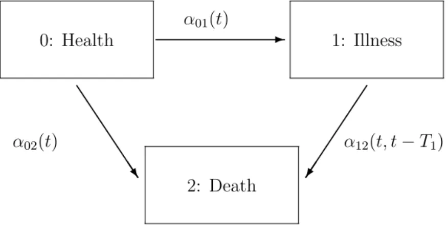
correspon-dence between multi-state processes and multivariate counting processes was studied in Commenges & G´egout-Petit (2006) where the advantage of rep-resenting multi-state processes as multivariate “basic” counting processes is highlighted. Multi-state models are often generated by p types of events, each type occurring just once. For instance the three-state illness-death model (see Figure 1) is generated by considering the events “illness” and “death” ; the five-state model considered by Commenges & Joly (2004) is generated by “dementia”, “institutionalization” and “death”. So these multi-state models
can be represented by a p-variate counting process N, each Nj making at
most one jump, and we will denote Tj the jump time of Nj.
2.2
Possible semi-parametric Models
A model for a multivariate counting process N = (Nj, j = 1, . . . , p) is
spec-ified for a given filtration {Ft} by its intensity λθ(t) = (λθj(t), j = 1 . . . , p)
under Pθ.
For efficient inference one has to make assumptions: often the Markov
assumption is made: the process is Markov if and only if λθ(t) is a function
of only time t and the indicator functions 1{Tj<t}, j = 1, . . . , p. An interesting
non-Markov model occurs if λθ(t) depends on the time elapsed since the last
jump of one of the components of N. If the intensities do not depend on the time t itself this defines a particular semi-Markov model (used for instance by Lagakos, Sommer & Zelen, 1978) that we will call “current-state” model because the transition intensities depend only on the time spent in the current state.
Completely parametric models are often too rigid but parametric assump-tions may be made for some parts of the model: thus a semi-parametric ap-proach, in which a great flexibility is preserved on some part of the model while some parametric assumptions are made for simplicity and easier
inter-pretation, is often attractive. In such an approach, λθ(t) will depend on a
certain number of functions on which no parametric assumptions are made, some of them representing baseline transition intensity functions, and param-eters which appear in modeling how these baseline intensities will be changed as a function of events that have happened.
Let us consider some possible three-state irreversible illness-death models; these models are Markov or semi-Markov. Any model of this type is described
by a bivariate counting process, N1 counting illness and N2 counting death.
The intensity of N1 necessarily takes the form λθ1(t) = 1{T1≥t}1{T2≥t}α01(t),
where α01(t) has the interpretation of the transition intensity toward illness.
The intensity of N2 can generally be written λθ2(t) = 1{T2≥t}[1{T1≥t}α02(t) +
1{T1<t}α12(t, t − T1)]. The function α02(t) has the interpretation of the
tran-sition intensity from health toward death (the mortality rate of healthy sub-jects). To avoid having to estimate non-parametrically a bivariate function
we may consider models in which α12(t, t − T1) depends on two univariate
functions h(t) and g(t − T1); for instance we may consider an additive model
α12(t, t − T1) = h(t) + g(t − T1) as in Scheike (2001).
Particular cases of this model are:
M1: g = 0: non-homogeneous Markov model; here h(t) has the
interpre-tation of α12(t), the transition intensity from illness toward death;
M2: h(t) = 0: current state model; here g(.) has the interpretation of a
random transition intensity from illness toward death;
M3: h(t) = α02(t): excess mortality model; here g(t − T1) has the
inter-pretation of an excess mortality due to illness as a function of time passed in the illness state.
If explanatory variables Zi(t) for subject i are available we may consider
different models for the dependence of the intensities on the Zi(.) (the
vari-ables are either external or internal and in the latter case the filtration must
be rich enough so that the processes (Zi(t)) be adapted); in particular a
mul-tiplicative structure (in the spirit of the proportional hazard model) or an additive structure (in the spirit of the Aalen additive model: Aalen, Borgan & Fekjær, 2001) could be considered. For instance a multiplicative structure for the explanatory variables could be:
αi
01(t) = α001(t) exp(β01Zi(t)),
αi02(t) = α002(t) exp(β02Zi(t)),
αi
12(t, t − T1) = α012(t, t − T1) exp(β12Zi(t)),
where α0
01(t), α002(t) and α012(t, t − T1) are baseline transition intensities (the
last one being generally random and in that case defined only on {t > T1}).
3
Likelihood and penalized likelihood for
count-ing processes
3.1
Likelihood ratios
The model specifies a family of probability measures {Pθ}θ∈Θ; consider a
reference probability measure P0 such that each Pθ is absolutely continuous
relatively to P0 (P0 may or may not belong to {Pθ}θ∈Θ). The likelihood ratio
on a σ-field X is defined by:
LPθ/P0 X = dPθ dP0 |X a.s., where dPθ
dP0|X is the Radon-Nikodym derivative of Pθ relatively to P0 on X .
Remark 1. All equalities involving likelihood ratios or conditional ex-pectations are a.s. equalities; this may not be recalled every time.
Remark 2. Often likelihoods are computed using a reference measure that is not a probability measure and is not even specified. Here we will make it explicit and take a probability measure, in which case the term ”likelihood
ratio” is warranted. If the reference probability P0 belongs to (Pθ)θ∈Θ then
there exist θ0 such that P0 = Pθ0 and we may write L
θ/θ0
X = L Pθ/P0
X .
One of the advantages of representing multi-state models in the frame-work of counting processes (such in as section 2.1) is the availability of Jacod’s formula for the likelihood ratio based on observation on [0, C] in the
filtra-tion {Gt} where Gt = G0 ∨ Nt, where Nt = σ(Nju, 0 ≤ u ≤ t). The model
is specified by the intensities λθ
j(t) of the Nj’s under Pθ. It is advantageous
to take as reference probability, a probability P0 under which the Nj’s are
independent with intensities λ0
j(t) = 1{Njt−=0}; equivalently the Tj’s are
inde-pendent with exponential distributions with unit parameter. Using Jacod’s formula (Jacod, 1975) the likelihood ratio for this reference probability is:
LPθ/P0 GC = L Pθ/P0 G0 NY.C r=1 λθ Jr(T(r)) exp(−Λ θ .(C)) p Y j=1 eTj∧C, (1)
where for each r ∈ {1, . . . , N.C}, Jr is the unique j such that ∆NjT(r) = 1; N.t = Pp j=1Njt, Λθ.(t) = Pp j=1Λθj(t), Λθj(t) = Rt
0 λθj(u)du. This formula allows
us to compute the likelihood for any multi-state model once we have written it as a multivariate counting process.
3.2
Families of penalized likelihood estimators
Consider models specified by a set of parameters θ = (g, β) where g(.) =
(gj(.), j = 1, . . . , K) is a vector of functions from < to < and β a
vec-tor of real parameters. For instance for the Markov illness-death model
θ = (α01(.), α02(.), α12(.), β) where the αhj are transition intensities and β is
a vector of regression coefficients. If no parametric assumptions are made about the functions to be estimated and if smooth estimators are favored, the two main approaches are sieve estimators, extending the so-called hazard regression of Kooperberg & Clarkson (1997) or using orthogonal expansions such as in M¨uller & Stadtm¨uller (2005), and penalized likelihood (Gu, 1996; Joly et al., 2002).
Suppose that the sample consists of n independent observations of
mul-tivariate counting processes Ni = (Ni
j, j = 1, . . . , p), i = 1, . . . , n represented
by GiCi; the likelihood ratio L
Pθ/P0
¯
On , where ¯On = ∨GiCi, is the product of
con-tributions computed with formula (1). A penalized log-likelihood is defined as: plκ ¯ On(θ) = log L Pθ/P0 ¯ On − J(θ, κ), (2)
where κ = (κj, j = 1, . . . , K) is a set of smoothing coefficients. It is common
to use a penalty based on the L2-norms of the second derivatives of the
unknown functions: J(g(.), κ) = K X j=1 κj Z (gj00)2(u)du.
The penalized likelihood defines a family of estimators of θ, (ˆθκ)κ∈<K+,
and thus a family of estimators of the probability Pθ, (Pθˆκ)κ∈<K+. Asymptotic
results have been given for particular cases (Cox & O’Sullivan, 1990; Gu, 1996; Eggermont & La Ricia, 1999, 2001).
Consider now the situation where we can choose between different basic assumptions for our model (such as Markov or semi-Markov assumptions), indexed by η = 1, . . . , m. Formally we could include η in θ. However we prefer
to formalize the problem in a way that is closer to intuition and practice: for each value of η and each κ we have a maximum penalized likelihood
estimator ˆθη
κ; thus we have a family of estimators of the probability specified
by (Pθˆη
κ)η=1,...,m;κ∈<K+. The problem is to choose one estimator in this family.
In the following we will include η in κ considering that κ indexes a family of estimators, thus unifying the problem of smoothing coefficient and model structure.
4
Penalized likelihood for coarsened at
ran-dom counting processes
4.1
Coarsening at random in the TCMP
Here we consider a general case of incomplete data: we recall the TCMP model proposed in Commenges & G´egout-Petit (2005) and we give a version of the coarsening at random condition CAR(TCMP) and the factorization theorem it implies, adapted to the case where the reference probability is outside of the model; also we exhibit a “reduced” model that we will use in the sequel. The TCMP can be considered for any stochastic process X; when X is a counting process the TCMP includes in particular extensions of the concepts of right-, left- and interval-censoring that have been defined for survival data, as well as a combination of these different types of censoring. Definition 1 (The time coarsening model for processes (TCMP)) A
TCMP is a scheme of observation for a multivariate process X = (X1, . . . , Xp)
specified by a multivariate response process R = (R1, . . . , Rp), where the
Rjt’s take values 0 or 1 for all j and t, such that Xjt is observed at time
t if and only if Rjt = 1, for j = 1, . . . , p; that is, the observed σ-field is
O = σ(Rt, R.Xt, t ≥ 0).
In the definition we denote R.Xt= (R1tX1t, . . . , RptXpt). A model for (X, R)
is a family of measures {Pθψ}(θ,ψ)∈Θ×Ψon a measurable space (Ω, F). X (resp.
R) takes values in a measurable space (Ξ, ξ) (resp. (Γ, ρ)). For us X and R will be p-dimensional c`adl`ag stochastic processes, so (Ξ, ξ) and (Γ, ρ) are
Skorohod spaces endowed with their Borel σ-fields. The parameter spaces Θ and Ψ need not be finite dimensional. We will assume that the measures in the family are equivalent. The processes X and R generate σ-fields X
and R, and we shall take F = X ∨ R. PθX is the restriction of Pθψ to X :
that is, the marginal probability of X does not depend on ψ. The addi-tional parameter ψ will be considered as a nuisance parameter. We assume a ”Non-Informativeness” assumption in the coarsening mechanism, which,
writing PX
θψ = Pθψ(.|X ) (a conventional notation for conditional
probabili-ties: Kallenberg, 2001), is :
PθX1ψ = PθX2ψ, a.s., for all θ1, θ2, ψ (3)
This is a conventional assumption (although it has not been expressed in this form) and means that the coarsening mechanism (conditionally on X) depends on a distinct (from the parameter of interest θ) , “variation indepen-dent” parameter ψ. Now we consider a family of equivalent probabilities Q
including in addition to {Pθψ}(θ,ψ)∈Θ×Ψ a family of possible reference
proba-bilities. Let P0 be one such probability; we denote by P0X its restriction to
X and by PX
0 the associated conditional probability given X . The likelihood
ratio is then LPθψ/P0 F = L Pθψ/P0 R|X L PθX/P0X X , where L Pθψ/P0 R|X is the conditional
likelihood of R given X . Note that with the non-informativeness assumption
LPθψ/P0
R|X does not depend on θ; we will note it L
P.ψ/P0
R|X to emphasize this fact.
LPθψ/P0
F is the full likelihood and L
Pθψ/P0
O the observed likelihood.
Definition 2 (CAR(TCMP)) We will say that CAR(TCMP) holds for
the couple (X, R) in Q if LP1/P0
R|X is O-measurable for all P1, P0 ∈ Q.
We will use the following result (which is an adaptation of Theorem 2 in Commenges & G´egout-Petit, 2005):
Theorem 1 (Factorization) If the couple (R, X) satisfies CAR(TCMP)
then we have LPθψ/P0 O = L P.ψ/P0 R|X EP0[L PθX/P0X X |O] and EP0[L PθX/P0X X |O] does not depend on PX 0 .
This factorization is a first step toward ignorability because for instance
it is the same value of θ which maximizes EP0[L
PθX/P0X
X |O] and which
maxi-mizes LPθψ/P0
O ; a slightly stronger condition is necessary for ignorability (see
Commenges & G´egout-Petit, 2005).
We can achieve a nicer result which will help simplifying notations in
section 5. If we knew the true conditional probability given X , PX
∗ , we
would use the following “reduced” model: {Pθ}θ∈Θ such that PθX = P∗X.
Definition 3 (Reduced model) Given a model {Pθ,ψ}(θ,ψ)∈Θ×Ψ such that
the restriction of Pθ,ψ to X is PθX for all θ and ψ, we call “reduced model“
the model {Pθ}θ∈Θ such as the restriction of Pθ to X is PθX and PθX = P∗X
for all θ, where PX
∗ is the true conditional probability given X .
Note that this reduced model is “reduced” in the sense that it is a smaller family than the original one; however it is a submodel only if the original
model was well-specified (P∗ ∈ {Pθ,ψ}(θ,ψ)∈Θ×Ψ). Taking a reference
proba-bility P0 such that P0X = P∗X we have that L
Pθ/P0
R|X = 1 a.s. Thus we have,
without additional assumption, LPθ/P0
O = EP0[L
PθX/P0X
X |O]. If CAR(TCMP)
holds EP0[L
PθX/P0X
X |O] does not depend on P0X = P∗X. That is, we can
com-pute the exact likelihood that we would like to comcom-pute if we knew PX
∗ ,
without in fact knowing it.
There remains in practice to compute EP0[L
PθX/P0X
X |O] for the observed
value of R and this is explained for the case of multistate processes in the next section.
4.2
Likelihood and penalized likelihood for counting
processes
The likelihood for the deterministic TCMP (that is in which the R’s are deterministic functions) and when X is a multivariate counting process has been given in Commenges & G´egout-Petit (2006). The observation in this
scheme is denoted by the σ-field O and we have O ⊂ GC, so that the observed
likelihood can be expressed as: LPθ/P0
O = EP0[L
Pθ/P0
GC |O]. The formula for the
likelihood follows from computation of this conditional expectation using the disintegration theorem (Kallenberg, 2001).
In the case of the stochastic TCMP when CAR(TCMP) holds we use the
reduced model {Pθ}θ∈Θso that the likelihood ratio is LPOθ/P0 = EP0(L
Pθ/P0
GC |O)
and EP0(L
Pθ/P0
GC |O) does not depend on P
X
0 ; with a slightly stronger condition
it can be computed in practice as if the TCMP was deterministic, using the formulae given in Commenges & G´egout-Petit (2006), with values of the responses functions r equal to what has been observed.
As for the penalized likelihood it can also be extended to the case where the observations are CAR(TCMP): the formula is the same as (2).
5
Choice between semi-parametric models:
ex-pected Kullback-Leibler loss
5.1
General theory
The problem of choice of an estimator among a family of estimators using expected Kullback-Leibler risk has been studied in particular by Hall (1987), van der Laan & Dudoit (2003), van der Laan, Dudoit & Keles (2004). Since our aim here is to choose an estimator of a probability measure among a family of estimators, this theoretical criterion is particularly relevant. We formalize this criterion in this general context and for incomplete observa-tions. Although the focus of the paper is on counting processes, the formalism developed in this section applies to more general processes, so we will call the process of interest X as in section 4.1.
Let us now model n i.i.d. random elements (Xi, Ri), i = 1, . . . , n. We
consider a measurable space ( ¯Ωn, ¯Xn, ¯Rn) where ¯Ωn= ×Ωi, ¯Xn= ⊗Xi, ¯Rn=
⊗Ri where the σ-fields for different i are independent. The probability
mea-sures on this space are the product meamea-sures. Finally we define full and
observed σ-fields Fi = Ri∨ Xi and Oi = σ(Rit, Rit.Xit, t ≥ 0) respectively.
The problem is to estimate θ. When Θ is a functional space a conventional
strategy is to define estimators (that is ¯On-measurable functions) depending
on a meta-parameter κ: ˆθ(κ, ¯On). κ may index nested models such as in sieve
estimators or may be a smoothing parameter such as in penalized likelihood or kernel estimators. According to statistical decision theory (Le Cam & Yang, 1990) we should choose an estimator which minimizes a risk function, the expectation of a loss function. In statistics we assume that there is
a true probability P∗. We do not make the assumption that P∗ belongs
to the model; this assumption would significantly reduce the scope of the
theory. Making the assumption that P∗ is equivalent to the probabilities of
the model, the most natural “all-purpose” loss function relatively to P∗ is
− log LPθXˆ /P∗X
Xn+1 (we note ˆθ = ˆθ(κ, ¯On)), where P∗X is the restriction of P∗ to
X . However the problem will be to “estimate” the risk, that is to find a
statistic ( ¯On-measurable) which takes values close to that risk (this is not
exactly an estimation problem because the target moves with n but we will use the word “estimate” for simplicity). It may be considered as intuitive
that a risk based on − log LPθXˆ /P∗X
Xn+1 will be very difficult to estimate; this is
why Liquet and Commenges (2004) suggested using the expectation of the
observed loglikelihood of the sample, a criterion they denoted ELL. The use of the stochastic TCMP and the CAR(TCMP) assumption allows us working in the more comfortable i.i.d. framework for incomplete data leading to more elegant and general results.
The straightforward loss function on On+1 is − log L
Pθ, ˆˆψ/P∗
On+1 . A difficulty
arises in that this loss function requires an estimator of ψ. Hopefully the CAR(TCMP) assumption allows us to construct a reduced model as in sec-tion 4.1 in which we can construct a loss funcsec-tion not depending on the
con-ditional probability given X , PX
∗ . The first step is to construct the reduced
model associated to the reference probability P∗. Then we have, by
apply-ing the result of section 4.1 to that case and to σ-fields Xn+1, Rn+1, On+1:
LPθ/P∗
On+1 = EP∗[L
PθX/P∗X
Xn+1 |On+1] and this does not depend on P
X
∗ . We can now
construct the loss function as − log LPθˆ/P∗
On+1 = − log EP∗[L
PθXˆ /P∗X
Xn+1 |On+1, ¯On];
note that we must add the conditioning on ¯Onbecause ˆθ is an ¯On-measurable
random variable.
The conditional expectation of this loss, or conditional risk, is CKLn =
EP∗[− log L
Pθˆ/P∗
On+1| ¯On] and can be interpreted as the Kullback-Leibler
diver-gence between Pθˆand P∗, since the Kullback-Leibler divergence of a
probabil-ity P1relatively to P∗over the σ-field On+1is KL(P1, P∗) = EP∗[− log L
P1/P∗
On+1].
Its expectation, or risk, EKLn= EP∗[− log L
Pθˆ/P∗
On+1], can be interpreted as the
expected Kullback-Leibler divergence over the σ-field On+1 of interest.
5.2
Case of observed explanatory variables
Explanatory variables are considered as stochastic processes Z = (Zt)t≥0.
We can then consider the process W = (X, Z). In the TCMP framework
we associate the response process R = (RX, RZ). The observed σ-field is
O = σ(Rt, R.Wt, t ≥ 0). With such a formulation there is no need of a
special theory for explanatory variables. However it is often the case that: i) the marginal law of Z is not of interest, but only the conditional law of X given Z is of interest; ii) Z is completely observed, that is, all the components
of RZ are identically equal to one (we will refer to this by writing RZ = 1).
Because of i) we consider the following parametrization of the model: the
model is defined by the family of probability measures (Pθγψ)θ∈Θ,γ∈Γ,ψ∈Ψ,
where Pθγψ is specified by PγZ, PψX ,Z and PθXZ , that is γ indexes the marginal
probability of Z, ψ the conditional probability given X and Z, and θ the
conditional probability of X given Z on which the interest focuses. We take
a reference probability P0and we assume that CAR(TCMP) holds for (W, R),
that is LPθγψ/P0
R|W is O-measurable; this is equivalent to L
Pθγψ/P0
RX|W O-measurable
(where RX is the σ-field generated by RX) because RZ = 1 (this can be
seen for instance by applying property vi) of Commenges & G´egout-Petit, 2005). In that case, if ii) holds, we can get rid of both nuisance parameters
ψ and γ for the likelihood inference on θ. This is a consequence of the
double-factorization theorem.
Theorem 2 (Double-factorization) Consider the process W = (X, Z),
where X is the process of interest, Z is a process of explanatory variables; R =
(RX, RZ) is the associated response process and we have RZ = 1. Consider
the family of equivalent probability measures Q = {{Pθγψ}θ∈Θ,γ∈Γ,ψ∈Ψ, Q0},
where Pθγψ is specified by PγZ, PθXZ and PψX ,Z, and where Q0 is a family of
possible reference probabilities; the restriction of Pθγψ on W is denoted PθγW.
Consider a reference probability P0 ∈ Q0. If the couple (W, X) satisfies
CAR(TCMP) in Q, then we have: LPθγψ/P0 O = L Pθγψ/P0 R|W L PγZ/P0Z Z EP0[L PθγW/P0W X |Z |O] (4) and 1. LPθγψ/P0
R|W depends neither on θ nor on γ and can be denoted L
P.ψW/P0
R|W ;
LPγZ/P0Z
Z depends neither on θ nor on ψ; L
PθγW/P0W
X |Z depends neither on
ψ nor on γ and can be denoted LPθ.W/P0W
X |Z ;
2. EP0[L
Pθ.W/P0W
X |Z |O] depends neither on P0X ,Z nor on P0Z.
Proof. Since CAR(TCMP) holds for (W, R) we can apply the (simple)
factorization theorem which gives: LPθγψ/P0
O = L Pθγψ/P0
R|W EP0[L
PθγW/P0W
W |O].
We next use the decomposition LPθγW/P0W
W = L PγZ/P0Z Z L PθγW/P0W X |Z and since LPγZ/P0Z Z is O-measurable (because L PγZ/P0Z Z is Z-measurable and Z ⊂ O)
we obtain (4). Point (1) is straightforward. Another way to express Point
(2) is that if we consider two probabilities P1 and P0 such that P0XZ = P1XZ
we have EP0[L
Pθ.W/P0W
X |Z |O] = EP1[L
Pθ.W/P1W
X |Z |O]. The proof is similar to that
of Theorem 1 given in Commenges & G´egout-Petit (2005).
We can now apply the trick of the reduced model of section 4.1 to this
context. If we knew the true conditional probability given (X , Z), PX ,Z, and
the true marginal probability P∗Z, we would use the reduced model {Pθ}θ∈Θ
such that PθX ,Z = PX ,Z
∗ and PθZ = P∗Z. Taking a reference probability
P0 such that P0X ,Z = P∗X ,Z and P0Z = P∗Z we have that LPR|X ,Zθ/P0 = 1 a.s.
Thus we have, without additional assumption, LPθ/P0
O = EP0[L
Pθ.W/P0W
X |Z |O].
If CAR(TCMP) holds EP0[L
Pθ.W/P0W
X |Z |O] does not depend on P0W = P∗W nor
on P0Z = P∗Z. That is, we can compute the exact likelihood that we would
like to compute if we knew PX ,Z
∗ and P∗Z, without in fact knowing them.
We can adapt now the same reasoning as in the previous section for defining the risk function for choosing estimators in the case where there are
explanatory variables. We assume that we have n i.i.d. triples (Xi, Zi, Ri),
where the stochastic processes Zi represent time-dependent explanatory
vari-ables. Assuming that CAR(TCMP) holds for (Wi, Ri), i = 1, . . . , n, with
Wi = (Xi, Zi) and using the reduced model we have that LOPθn+1/P∗ = EP∗[L
Pθ.W/P∗W
Xn+1|Zn+1|On+1]
depends neither on PX ,Z
∗ nor on P∗Z. We define the loss function as before
as − log LPθˆ/P∗
On+1 = − log EP∗[L
Pθ.Wˆ /P∗W
Xn+1|Zn+1|On+1, ¯On] and the risk function as
EKLn = EP∗[− log L
Pθˆ/P∗
On+1].
6
Choice between semi-parametric models:
like-lihood cross-validation
6.1
Estimating EKL
nby likelihood cross-validation
Making the assumption that CAR(TCMP) holds for (Xi, Ri), i = 1, . . . , n we
use a reduced model based on a reference probability P0; then the observed
likelihood ratio is LPθ/P0
¯
On . If there are explanatory variables, we assume that
CAR(TCMP) holds for (Wi, Ri), i = 1, . . . , n, we use the reduced model and
we still denote the observed likelihood LPθ/P0
¯
On .
Now we are seeking an “estimator” for our criterion EKLn. We consider
the leave-one-out likelihood cross-validation criterion as a possible “estima-tor”. It is defined as:
LCVn(ˆθ(.; .), κ, ¯On) = − 1 n n X i=1 log LPOθ(κ, ¯ˆi On|i)/P0,
where ¯On|i = ∨j6=iOj.
A first property, bearing on expectation of LCV is:
Lemma 1 EP∗[LCVn(ˆθ(.; .), κ, ¯On)] = EKLn−1(ˆθ(.; .), κ) − KL(P0, P∗). Proof. We have EP∗[LCVn(ˆθ(.; .), κ, ¯On)] = −EP∗[log L Pθ(κ, ¯ˆ On|i)/P0 Oi ] = −EP∗[log L Pθ(κ, ¯ˆ On|i)/P∗ Oi − log L P∗/P0 Oi ] = EKLn−1(ˆθ(.; .), κ) − KL(P0, P∗).
So, using LCVn for the choice of κ we are using an unbiased
estima-tor of EKLn−1: indeed, since KL(P0, P∗) does not depend on κ, we have
EP∗[LCVn(ˆθ(.; .), κ2, ¯On)]−EP∗[LCVn(ˆθ(.; .), κ1, ¯On)] = EKLn−1(ˆθ(.; .), κ2)−
EKLn−1(ˆθ(.; .), κ1). Thus LCV estimates a difference in EKL without the
assumption that the true probability belongs to the model. Moreover we conjecture that the optimal properties obtained by Hall (1987) and van der Laan, Dudoit & Keles (2004) extend under certain assumptions to the gen-eral context considered here and that cross-validation will effectively be able to choose between semi-parametric multi-state models.
6.2
Computational algorithm
6.2.1 Approximation of the solution of the penalized likelihood
The penalized likelihood estimator ˆθκ is the set of functions and parameters
which maximize plκ(θ). In general it is not possible to compute ˆθκanalytically
so the ˆgκ
k are approximated, for instance by splines. With this
approxima-tion the optimisaapproxima-tion problem becomes a standard maximizaapproxima-tion on a finite number of parameters. (Note that the number of knots in the spline repre-sentation is limited only by computational issues: the smoothness of the final
estimator for the gk(.) is controlled by κ in the penalized likelihood, not by
the number of knots). Calling γ the set of new parameters (including β and the set of spline parameters) we are led to maximizing:
plO¯n = plκO¯n(γ) = LγO¯n− J(γ, κ), (5)
where LγO¯n = log Lγ/PO¯n0. We note ˆγ = ˆγ( ¯On, κ) = argmaxγ(plOκ¯n(γ)).
6.2.2 Approximation of LCV
Since LCVn (that we will note simply LCV from now on) is particularly
computationally demanding when n is large an approximate version LCV
has been proposed by O’Sullivan (1988) for estimation of the hazard function in a survival case and adapted by Joly et al. (2002) to the case of interval-censored data in an illness-death model. We may still extend it to a general framework valid for any penalized likelihood depending on a vector of real
parameters γ. We note LCV = −n−1Pn
i=1L
ˆ
γ−i
Oi , where ˆγ−i = ˆγ( ¯On|i, κ). The
first order development of Lγˆ−i
Oi around ˆγ yields: Lγˆ−i Oi ≈ L ˆ γ Oi + (ˆγ−i− ˆγ) Tdˆ i, (6) where ˆdi = ∂LγOi
∂γ |ˆγ. The first order development of ∂plγOn|i¯ ∂γ |ˆγ−i gives: ˆ γ−i− ˆγ ≈ −Hpl−1On|i¯ ∂plγO¯n|i ∂γ |ˆγ, where HplOn|i¯ = ∂2pl¯ On|i
∂γ2 |ˆγ, and more generally Hg = ∂
2g
∂γ2|ˆγ. At first order
HplOn|i¯ ≈ HplOn¯ . From the equality plO¯n(γ) = plO¯n|i(γ) + L
γ Oi we deduce by taking derivatives: 0 = ∂pl γ ¯ On|i ∂γ |ˆγ + ˆdi
which finally yields:
ˆ
γ−i− ˆγ ≈ Hpl−1On¯ dˆi,
which inserted in (6) gives:
Lγˆ−i ¯ Oi ≈ L ˆ γ ¯ Oi + ˆd T i Hpl−1On¯ dˆi.
Substituting this expression in the expression of LCV we obtain:
LCV ≈ LCVa1 = −n −1[Lγˆ ¯ On + n X i=1 ˆ dTi Hpl−1¯ On ˆ di].
Using the fact that both n−1Pn
i=1dˆidˆTi and −n−1HLOn¯ tend towards the
in-dividual information matrix I = −EP∗(HLOi) we get another approximation:
LCV ≈ LCVa = −n−1[LˆγO¯n− Tr(Hpl−1On¯ HLOn¯ )].
This expression looks like an AIC criterion and there are arguments to
in-terpret Tr[H−1
plOn¯ HLOn¯ ] as the model degree of freedom. For instance, if there
is no penalty (J = 0), HplOn¯ = HLOn¯ so that the correction term in LCVa
reduces to dim(γ), that is LCVa reduces to AIC.
If κ is a scalar minimization of LCVacan be done by standard line-search
algorithms; if it is a vector, a grid algorithm can be used (Joly et al., 2002).
7
Simulation study
7.1
Description and main result
We did a simulation study to illustrate the ability of LCV to choose the right model structure; the possibilities were the Markov structure and the
semi-Markov current-state structure, respectively models M1 and M2 in section
2.2. The best model is not always the right model, especially in the case where the right model is larger than alternative models. Here, the model 1 and model 2 structures are of similar complexities, so we think that the right model should be the best model.
We considered two particular models (or probability measures, M1 ∈ M1
and M2 ∈ M2). For both M1 and M2 the transition intensities toward
illness, α01(t), and death, α02(t), were taken equal to the hazard function of
Weibull distributions, namely: pγptp−1 with parameters (p = 2.4; γ = 0.05)
and (p = 2.5; γ = 0.06) respectively. Models M1 and M2 differed by the
intensity of N2 for t > T1, that is the mortality rate of diseased. For M1 the
mortality rate was defined by h(t) and was a Weibull hazard function with
parameters (p = 2.6; γ = 0.08); for M2 it was defined by g(t − T1) which
was equal to a Weibull hazard function with parameters (p = 1.5; γ = 0.2). For each subject we generated an ignorable TCMP observation scheme by
generating R1 and R2 independently from N1 and N2. In intuitive terms R1
and R2 were constructed to represent a situation where N1 was observed at
discrete times and N2 was observed in continuous time and possibly
right-censored (the same as in the application). For each subject we generated visit
times Vj at which N1 was observed as Vj = Vj−1+ 2 + 3Uj, where the Uj’s
were independent uniform [0, 1] random variables and observation of both N1
and N2 was right-censored by a variable C which had a uniform distribution
on [2, 52]. We had R1(t) = 1{t<C}
P
j=11{t=Vj} and R2(t) = 1{t<C}. To take
into account the discrete-time observation scheme on one component we used formula (13) of Commenges & G´egout-Petit (2006).
We generated 100 replicas of samples N1 and N2 from M1 and M2; each
sample had n = 1000 subjects. For each replica, the three functions
deter-mining the model (α01(.), α02(.) for both models and h(.) for M1 and g(.)
for M2) were estimated by penalized likelihood while the parameter ˆη
(de-termining model structure) and the smoothing coefficients ˆκ = (ˆκ1, ˆκ2, ˆκ3)
which minimized LCV were determined.
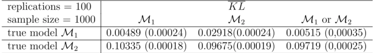
The first result is that when the Markov model was generated it was chosen in 99 cases out of 100; when the semi-Markov model was generated it was chosen in 93 cases out of 100. This shows that LCV does a good job in picking the right model structure. Table 1 shows the distance in term of the risk EKL (the avrage Kullback-Leibler loss is an estimate of EKL) between the estimated models and the true model: choosing the model structure by
LCV incurs a very slight additional risk (of order 10−4) as compared to
knowing the true model but a lower risk as compared to choosing the wrong
model; in the latter case the additional risk is of order 10−2.
This result must not be falsely interpreted. First the discrimination prop-erties of LCV depends on many parameters and particularly on the quantity of information available in the samples. Second and even more important the aim of estimator choice is not to choose the right model but to choose the best estimator. The choice between the two structures depends on how “far” the two models are. If the models are “close” it is of course more difficult to discriminate between them, but at the same time it becomes less important to choose the right one. For instance the homogeneous Markov model be-longs to both structures so it is possible by small perturbations of this model to construct two models, one Markov and one semi-Markov, which are very near in term for instance of Kullback-Leibler divergence.
7.2
Study of the variability of LCV
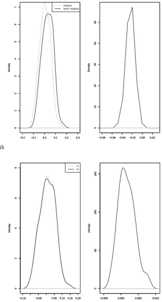
In this section we exploit the above simulation study to explore the variability
of LCV . We have estimated from the 100 replicas from M1 the density of
LCV (ˆκ) assuming M1 and assuming M2. The upper-left panel of Figure 2
displays these estimated densities: there seems to be little difference between the two, so one may wonder whether LCV can be of any use for choosing between the two model structures. However when we look at the density
of the difference between LCV (ˆκ) for M1 and M2 we see that most of the
mass is in the negative values, so that most of the time the true model M1
will be chosen. Similarly the lower panels show the estimated densities of
LCV , assuming M1, for two different values κ1 and κ2 of the smoothing
coefficient. Here the two densities are nearly undistinguishable while the density of the difference is clearly shifted toward positive values. Another
way to examine this issue is to look at the standard deviations of LCV (κ1),
LCV (κ2) and LCV (κ2)-LCV (κ1): we estimated these values (under M1)
to be 0.048, 0.048 and 0.0024 respectively. Thus the standard deviation of
the difference is about twenty times less than that of LCV for κ1 or κ2.
This explains why LCV does a good job in model choice in spite of its large variability.
7.3
Quantitative interpretation of Kullback-Leibler
di-vergences
For practical use of the method proposed in this paper it is important to have an idea of whether a particular EKL value, or a difference of EKL values or their LCV estimators are large or not. As in more conventional situations we must distinguish the interpretational issue from statistical issues. For instance in the conventional situation of a regression parameter the statistical issues beyond the point estimation of the parameter are to test the hypothesis of a null value of the parameter and to give a confidence interval for this parameter; the interpretational issue is to be able to assess the importance of the effect on the variable of interest. For instance in an epidemiological application using a Cox model we would consider the exponential of the parameter and interpret it as a relative risk, considering that a value of 1.1, 2, 5 would correspond to a small, moderate, large increase of risk respectively. We would like have a guide toward such an interpretation when manipulating
EKL values.
Since EKL is an expected Kullback-Leibler divergence it can be
inter-preted as a Kullback-Leibler divergence. So let us try to interpret KL( ˜P , P∗).
If we consider that P∗ is the true probability this means that we will make
errors by evaluating the probability of an event A by ˜P (A) rather than by
P∗(A). For instance we may evaluate the relative error re( ˜P (A), P∗(A)) =
P∗(A)− ˜P (A)
P∗(A) . Consider the typical event on which ˜P (A) will be under-evaluated
defined as: A = {ω : LP /P˜ ∗ < 1}. In order to obtain a simple formula
relating KL( ˜P , P∗) to the error on P∗(A) we consider the particular case
P∗(A) = 1/2 and LP /P˜ ∗ constant on A and AC (or equivalently we
com-pute KL for a likelihood defined on σ(A)). In that case we easily find:
r ( ˜P (A), P (A)) =
q
1 − e−2KL( ˜P ,P∗)≈
q
2KL( ˜P , P ), the approximation
ing valid for small KL value. For KL values of 10−1, 10−2, 10−3, 10−4, we
find that re( ˜P (A), P∗(A)) is equal to 0.44, 0.14, 0.045 and 0.014, errors that
we may qualify as “large”, “moderate”, “small” and “negligible”.
As an example the KL divergence of a double exponential relative to a
normal distribution with same mean and variance is of order 10−1 leading to
a “large” re( ˜P (A), P∗(A)). In the previous simulation study we have found
that choosing the wrong model leads to an increase of the risk of order 10−2
which is “moderate”, while choosing the model by LCV leads to and increase
of order 10−4 which may be qualified as “negligible”.
8
Application on dementia
We illustrate the use of this general approach using the data of the Paquid study (Letenneur et al., 1999), a prospective cohort study of mental and physical aging that evaluates social environment and health status. The tar-get population consists of subjects aged 65 years and older living at home in southwestern France. The diagnosis of dementia was made according to a two-stage procedure: the psychologist who filled the questionnaire screened the subjects as possibly demented according to DSM-III-R or not; subjects classified as positive were later seen by a neurologist who confirmed (or not) the diagnosis of dementia and made a more specific diagnosis, assessing in particular the NINCDS-ADRDA criteria for Alzheimer’s disease. Subjects were re-evaluated 1, 3, 5, 8, 10 and 13 years after the initial visit. Subjects already demented at the initial visit were removed from the sample, a se-lection condition which is easily taken into account by using a conditional likelihood as mentioned in Commenges & G´egout-Petit (2006). The sam-ple consisted of 3673 subjects, 1540 men and 2133 women. Previous work (Commenges et al., 2004) has shown that the effect of gender on the risk of dementia is neither multiplicative nor additive; in fact the dynamics of ageing is so different between men and women that it is safer to perform completely separate analyses. For the purpose of this illustration we ana-lyzed only women. During the 13 years of follow-up 396 incident cases of dementia and 835 deaths were observed. We wish to jointly model dementia and death, an approach conventionally referred to as the illness-death model; the model can be graphically described as in figure 1, where the mortality
rate of demented is noted α12(t, t − T1) to emphasize the fact that it may
depend on both age t and time since onset of dementia t − T1; we assume
that the transition intensities do not depend in addition on universal (or calendar) time. Note that dementia is observed in discrete time while death is observed in continuous time. One effect of the observation scheme is that we miss a certain number of dementia cases: we do not observe a dementia case which has happened when the subject develops dementia and dies be-tween two planned visits. This scheme of observation and the likelihood for it are explained heuristically in Commenges et al. (2004) and rigorously in Commenges & G´egout-Petit (2006).
We tried the three model structures depicted in section 2.2. We took as reference probability the homogeneous Markov model fitted to the data. Thus LCV estimated the change in EKL when going from the homoge-neous Markov maximum likelihood estimator to another estimator. The values of the best LCV criteria for the different model structures were:
Non-homogeneous Markov model (M1): -0.2182; Current state model (M2):
-0.2100; Excess mortality model (M3): -0.2180. This means for instance that
the best penalized likelihood estimator in the non-homogeneous model has an estimated expected Kullback-Leibler divergence (EKL) relative to the true model which is smaller by 0.2182 than the homogeneous Markov esti-mator. The best LCV was found for the non-homogeneous Markov model. However the best “excess mortality” estimator is not far from the best non-homogeneous estimator, while the current state estimator seems to be farther.
In terms of the interpretation of section 7.3 the difference between M2 and
M1 is moderate while that between M3 and M1 is negligible.
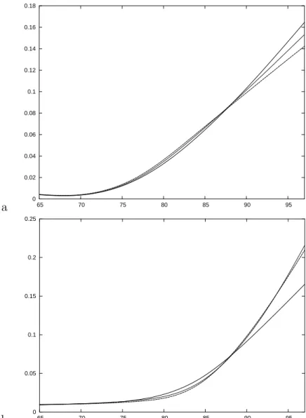
We compared graphically the best estimators found for the three model structures considered. Figure 3 shows the three estimators for the age-specific
incidence of dementia (α01) and the mortality rates of non-demented
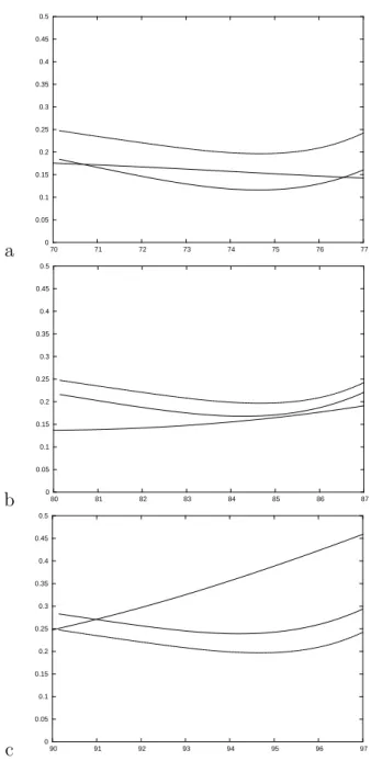
respec-tively: the three estimators are very close for incidence of dementia; there is a certain difference between the Markov model and the two semi-Markov models for mortality rates of non-demented above 90. Figure 4 displays the three estimators of the age-specific mortality rates of demented for different ages at onset of dementia, respectively 70, 80 and 90. Here the patterns are different although the magnitude of these estimators are similar. In partic-ular the current-state estimator is the same for the three ages at onset (by assumption) while we see a marked increase of mortality for age at onset of 90 in the non-homogeneous Markov estimator. From a qualitative point of view we may say that the three estimators agree for ages at onset of 70 and 80: the mortality rate for demented women does not vary much either with time since onset of dementia or with age at onset, and is around 0.2.
9
Conclusion
We have extended the expected Kullback-Leibler risk function (EKL) for estimator choice from generally coarsened observations of a stochastic pro-cess, including in the case of explanatory variables. We have suggested that this could be used for choosing both smoothing coefficients and model struc-ture; we have suggested that EKL could be approached by LCV and we have given a general approximation formula for the leave-one-out LCV . The simulation presented showed that the LCV did a good job in discriminating between model structures. The approach was illustrated in the problem of choosing between different additive illness-death models. The approach is in fact quite general and could be applied for instance to the choice between additive and multiplicative models.
Other choices might have been done: other loss functions, families of estimators and ways of estimating the risk function might have been cho-sen. However the choices we have done for the different components of the approach are adapted to the problem and fit well together. For instance the CAR(TCMP) assumption allows us to eliminate the nuisance param-eters from the chosen loss function; LCV is a natural estimator of EKL; penalized likelihood yields a flexible family of smooth estimators for which an approximation of LCV can easily be computed. The approach yields an operational tool for exploring complex event histories, for instance in the domain of ageing.
There are many open problems and useful developments would be: find-ing a better algorithm for minimizfind-ing LCV over multiple smoothfind-ing parame-ters; studying the variance of LCV (see Bengio & Grandvalet, 2004); finding asymptotic properties of the estimators chosen by minimizing LCV .
10
References
Aalen, O. (1978). Nonparametric inference for a family of counting processes.
Ann. Statist. 6, 701-726.
Aalen, O., Borgan, O. & Fekjaer (2001). H. Covariate Adjustment of Event Histories Estimated from Markov Chains: The Additive Approach.
Biomet-rics 57, 993-1001.
Aalen, O. & Johansen S. (1978). An empirical transition matrix for
homogenous Markov chains based on censored observations. Scand. J.
Statist. 5, 141–150.
Andersen, P.K, Borgan Ø, Gill RD & Keiding N. (1993). Statistical Models
Based on Counting Processes. New-York: Springer-Verlag.
Bengio, Y. & Grandvalet, Y. (2004). No unbiased estimator of the variance of the K-fold cross-validation. Journal of Machine Learning Research 5, 1089-1105.
Commenges, D. & G´egout-Petit, A., (2005). Likelihood inference for
incom-pletely observed stochastic processes: ignorability conditions. arXiv:math.ST/0507151. Commenges, D. & G´egout-Petit, A. (2006). Likelihood for generally
coars-ened observations from multi-state or counting process models. Scand. J.
Statist., in press.
Commenges, D. & Joly, P. (2004). Multi-state model for dementia, institu-tionalization and death. Commun. Statist. A 33, 1315-1326.
Commenges, D., Joly, P., Letenneur, L. & Dartigues, JF. (2004). Incidence and prevalence of Alzheimer’s disease or dementia using an Illness-death model. Statist. Med. 23, 199-210.
Cox, D. & O’Sullivan, F. (1990). Asymptotic analysis of penalized likelihood and related estimators. Ann. Statist. 18, 1676-1695.
Eggermont, P. & LaRiccia, V. (1999). Optimal convergence rates for Good’s nonparametric likelihood density estimator. Ann. Statist. 27, 1600-1615. Eggermont, P. & LaRiccia, V. (2001). Maximum penalized likelihood
estima-tion. New-York: Springer-Verlag.
Gill, R. D., van der Laan, M. J. & Robins, J.M. (1997). Coarsening at ran-dom: characterizations, conjectures and counter-examples, in: State of the
Art in Survival Analysis, D.-Y. Lin & T.R. Fleming (eds), Springer Lecture
Notes in Statistics 123, 255-294.
Good, I.J. & Gaskins, R.A. (1971). Nonparametric roughness penalty for probability densities. Biometrika 58, 255-277.
Gu, C. (1996). Penalized likelihood hazard estimation: a general procedure.
Statistica Sinica 6; 861-876.
Hall, P. (1987). On Kullback-Leibler loss and density estimation. Ann.
Statist. 15, 1491-1519.
Hougaard, P. (2000). Analysis of multivariate survival data. New York: Springer.
Jacod, J. (1975). Multivariate point processes: predictable projection; Radon-Nikodym derivative, representation of martingales. Z. Wahrsch. verw. Geb. 31, 235-253.
Joly, P. & Commenges, D. (1999). A penalized likelihood approach for a progressive three-state model with censored and truncated data: Application to AIDS. Biometrics 55, 887-890.
Joly, P., Commenges, D., Helmer, C. & Letenneur, L. (2002). A penalized likelihood approach for an illness-death model with interval-censored data: application to age-specific incidence of dementia. Biostatistics 3, 433- 443. Kallenberg, O. (2001). Foundations of modern probabilities. Springer Verlag, New-York.
Kooperberg C. & Clarkson DB. (1997). Hazard regression with interval-censored data. Biometrics 53, 1485-1494.
Lagakos, S.W., Sommer, C.J. & Zelen, M. (1978). Semi-Markov models for partially censored data. Biometrika 65, 311-317.
Le Cam, L. & Yang, G. (2000). Asymptotics in Statistics. New-York: Springer-Verlag.
Letenneur, L., Gilleron, V., Commenges, D., Helmer, C., Orgogozo, JM. & Dartigues JF. (1999). Are sex and educational level independent predictors of dementia and Alzheimer’s disease ? Incidence data from the PAQUID project. J. Neurol. Neurosurg. Psychiatr. 66, 177-183.
Liquet, B. & Commenges, D. (2004). Estimating the expectation of the log-likelihood with censored data for estimator selection. Lifetime Data Analysis 10, 351-367.
Liquet, B., Saracco, J. & Commenges, D. (2006). Selection between
portional and stratified hazards models based on expected log-likelihood.
Computational Statistics, in press.
Liquet, B., Sakarovitch, C & Commenges, D.(2003). Bootstrap choice of estimators in parametric and semi-parametric families: an extension of EIC.
Biometrics 59, 172-178.
M¨uller, HG. & Stadtm¨uller, U. (2005). Generalized functional linear models.
Ann. Statist. 33, 774-805.
O’Sullivan, F. (1988). Fast computation of fully automated log-density and log-hazard estimators. SIAM Journal on Scientific and Statistical Computing 9, 363-379.
Ramlau-Hansen, H. (1983). Smoothing counting process intensities by means of kernel functions. Ann. Statist. 11, 453,466.
Scheike, T. (2001). A generalized additive regression model for survival anal-ysis. Ann. Statist. 29, 1344-1380.
van der Laan, M. & Dudoit, S. (2003). Unified cross-validation methodol-ogy for selection among estimators and a general cross-validated adaptive epsilon-net estimator: finite sample oracle inequalities and examples. Berke-ley Division of Biostatistics working paper series, paper 130.
van der Laan, M., Dudoit, S. & Keles, S. (2004). Asymptotic optimality of likelihood-based cross-validation. Statistical Applications in Genetics and Molecular Biology 3, Issue 1, article 4.
Daniel Commenges, INSERM U 875; Universit´e Victor Segalen Bordeaux 2, 146 rue L´eo Saignat, Bordeaux, 33076, France
E-mail: daniel.commenges@isped.u-bordeaux2.fr
replications = 100 KL
sample size = 1000 M1 M2 M1 or M2
true model M1 0.00489 (0.00024) 0.02918(0.00024) 0.00515 (0,00035)
true model M2 0.10335 (0.00018) 0.09675(0.00019) 0.09719 (0,00025)
Table 1: Average Kullback-Leibler loss KL and the corresponding standard
errors (numbers in the parentheses) for estimators chosen by LCV
0: Health 1: Illness 2: Death α01(t) α02(t) α12(t, t − T1) -J J J J J J J ^ À
Figure 1: The illness-death model. t: age; T1: age of onset of illness.
a −0.2 −0.1 0.0 0.1 0.2 0.3 0 1 2 3 4 5 6 7 Density −0.2 −0.1 0.0 0.1 0.2 0.3 0 1 2 3 4 5 6 7 Density markov semi−markov −0.08 −0.06 −0.04 −0.02 0.00 0.02 0 10 20 30 40 50 Density −0.08 −0.06 −0.04 −0.02 0.00 0.02 0 10 20 30 40 50 Density b −0.15 −0.05 0.050.100.150.20 0 2 4 6 8 Density −0.15 −0.05 0.050.100.150.20 0 2 4 6 8 Density κ1 κ2 −0.005 0.000 0.005 0.010 0 50 100 150 Density −0.005 0.000 0.005 0.010 0 50 100 150 Density
Figure 2: Kernel density estimation of LCV (left) and of differences of LCV (right) for a) Markov and semi-Markov choices, b) for two different values of the smoothing parameter; in all cases the true model is Markov.
a 0 0.02 0.04 0.06 0.08 0.1 0.12 0.14 0.16 0.18 65 70 75 80 85 90 95 b 0 0.05 0.1 0.15 0.2 0.25 65 70 75 80 85 90 95
Figure 3: Incidence of dementia (a) and mortality (b) for non-demented women for the three models. Continuous line: non-homogeneous Markov model; dashed line: current state model; dotted line: excess mortality model
a 0 0.05 0.1 0.15 0.2 0.25 0.3 0.35 0.4 0.45 0.5 70 71 72 73 74 75 76 77 b 0 0.05 0.1 0.15 0.2 0.25 0.3 0.35 0.4 0.45 0.5 80 81 82 83 84 85 86 87 c 0 0.05 0.1 0.15 0.2 0.25 0.3 0.35 0.4 0.45 0.5 90 91 92 93 94 95 96 97
Figure 4: Mortality of demented women for the three models: Continuous line: non-homogeneous Markov model; dashed line: current state model; dotted line: excess mortality model. Age at onset of dementia: a): 70; b): 80; c): 90.