The development of a three-degree-of-freedom vibration control system test facility

The Development of a Three-Degree-of-Freedom

Vibration Control System Test Facility

by

Travis Lee Hein

Submitted to the Department of Mechanical Engineering

in partial fulfillment of the requirements for the degree of

Bachelor of Science and Master of Science in Mechanical Engineering

at the

MASSACHUSETTS INSTITUTE OF TECHNOLOGY

May 1994

©

Massachusetts Institute of Technology 1994. All rights reserved.

A uthor ...

....

. ...

...

Department of Mechanical Engineering

May 6, 1994

Certified by..

...-..-.

...

Jamie W. Burnside

Company Supervisor

Thesis Supervisor

Certified by... ,-...

Ent

James K. Roberge

Professor of Electrical Engineering

Thesis Supervisor

David L. Trumper

Professor of Mechanical Engineering

"-

Thesis Supervisor

LIBRAP

Accepted by

...

Ain

A. Sonin

Chairman, Departmental Committee on Graduate Students

Certified

I,

The Development of a Three-Degree-of-Freedom Vibration

Control System Test Facility

by

Travis Lee Hein

Submitted to the Department of Mechanical Engineering on May 6, 1994, in partial fulfillment of the

requirements for the degree of

Bachelor of Science and Master of Science in Mechanical Engineering

Abstract

In this thesis, I developed a test facility which simulates the operational vibration of aircraft and spacecraft in three degrees-of-freedom: one linear and two angular degrees-of-freedom over a frequency range of 10 to 200 Hz. The purpose of the test facility is to evaluate the performance of control algorithms designed to actively reject a disturbance environment created by the facility.

Three electrodynamic shakers coupled to a common payload mounting platform provided this disturbance environment. The main focus of this project was upon the mechanical design and finite element analysis of the components which couple the three actuators to the mounting platform. Specially-designed flexures were utilized instead of conventional ball-and-socket joints to eliminate friction from the system.

A center post composed of a linear bearing, suspension system, and another flexure

system was designed and fabricated to improve the vibrational performance of the system.

A frequency domain, feed-forward controller was used to control the output of the

shakers, to ensure a payload mounted on the platform will be subjected to the desired power spectral density profiles specified by the user.

The controller was found to be able to track the three degrees-of-freedom to within ± 1 dB. The main limitation to the accuracy of the system was determined to be the ability of the controller to record accurate transfer functions of the three controlled degrees-of-freedom. The mechanical characteristics of the facility do not limit the current controller tracking abilities. Furthermore, the mechanical design of the test facility allow the operational frequency range to be increased to approximately 400

Hz.

Thesis Supervisor: Jamie W. Burnside Title: Company Supervisor

Title: Professor of Electrical Engineering Thesis Supervisor: David L. Trumper Title: Professor of Mechanical Engineering

Acknowledgments

I would like to thank first my thesis advisors, Professor Roberge and Professor Trumper, who have always provided me support and excellent guidance through the course of my thesis.

Through my work at Lincoln Laboratory, I feel that I have had the opportunity to work with people of the highest technical ability. Many thanks go out to those whose advice was extremely valuable: Al Pillsbury, Paul Martin, and Alley Catyb.

I am deeply indebted to the engineers and technicians of Group 76 for their advice, support, and help. I would especially like to thank Jamie Burnside for his insightful advice and motivation. I would also like to thank Paul Pepin for his expert design advice, mechanical drawings, and lessons in machining. This project could not have been accomplished without your help.

I would finally like to thank Sean Olson for helping me to stay focused upon the big picture and to keep this project in the proper perspective.

Contents

1 Introduction 11

1.1 Motivation for Control Systems Test Facility . ... 11

1.2 Overview of Control Systems Test Facility . ... 13 1.3 Performance Specifications of Test Facility . ... 16

2 Literature Review 19

2.1 Beam Steering Mirror Projects ... 19

2.2 Syminex Three Degree-of-Freedom Shaker System . ... 24

2.3 Laser Line-of-Sight Control ... 26

3 Fundamental Issues 29

3.1 Six Degree-of-Freedom Model ... 29 3.2 Vibrational Coupling ... 35 3.2.1 Coupling Between Actuated Degrees-of-Freedom ... 36

3.2.2 Coupling Caused by Mechanical Components of System . ... 37

3.3 Control Issues ... 37

3.3.1 Three Single-Input Single-Output Loops About Each DOF . . 38

3.3.2 I*star Controller Alone ... 42

3.3.3 Three Single-Input Single-Output Loops About Each Shaker . 43 4 Component Characterization and Design 46 4.1 Coordinate Transformation Circuit ... .. 46 4.2 Electrodynamic Shakers ... . 48 4.3 Vibrational Mounting Platform ... .. 52

4.4 Four-Axis Flexures . . . . 4.4.1 4.4.2 4.4.3 4.4.4 4.4.5 4.5 Center 4.5.1 4.5.2 4.5.3 4.5.4 Design Goals . . . . Design of Flexures . . . . Finite Element Model . .

Experimental Performance Alternative Solutions . . . Post . . . . .. . . . . Design Goals . . . .

Design of Center Post . . Experimental Performance Alternative Solutions . . . 4.6 Accelerometers . . . .

5 Controller Results

5.1 I*star Performance with the Center Post . . . . 6 Conclusions

6.1 Torsional Mode of System ...

6.2 Rocking Modes of System ...

6.3 Recommendations for Improving I*star Performance . . . . 6.4 Recommendations for Development of a Similar Test Facility . . . . .

A Decoupling Process

B Drawing of Four-Axis Flexure

C Drawings of Center Post Design

94 94 105 105 106 106 107 109 111 113

List of Figures

1-1 Disturbance and Shaker Axes ... 14

1-2 Photograph Depicting Shaker Configuration . ... 15

1-3 Block Diagram of ACCEL ... 17

2-1 2m Aperture Beam Steering Mirror . . . . .. . . . . 20

2-2 Flexible Piston for Beam Steering Mirror . . . . 21

2-3 Exploded View of HBSM ... .23

2-4 Diagram of Syminex 3 DOF Shaker System . . . ... . . . 25

2-5 Diagram of Single Degree-of-Freedom Line-of-Sight Experiment . . . 27

2-6 Sketch of Right Angle Flexure Hinge . . . ... . . . . 27

3-1 Six Degree-of-Freedom Model ... 30

3-2 Ideal Transfer Function .... . ... ... .. . ... 39

3-3 General Closed Loop Block Diagram Including Disturbance and Mea-surement Noise Inputs ... 40

3-4 Closed Loop Block Diagram of Single-Input Single-Output Control Schem e . . . .. . . .. . . .. . .. . . .. .. . .. . . . .. . 41

3-5 Compensated Closed Loop Block Diagram . . . . 42

3-6 Compensated Ideal Transfer Function . ... 43

3-7 I*star Controller Block Diagram ... 44

3-8 Three SISO Loops About Each Shaker . . . . 44

3-9 Two Degree-of-Freedom Model ... .45

4-2 4-3 4-4 4-5 4-6 4-7 4-8 4-9 4-10 4-11 4-12 4-13 4-14 4-15 4-16 4-17 4-18 4-19 4-20 4-21 4-22 4-23 4-24 4-25 4-26 4-27 4-28 4-29

Bare Shaker Transfer Function . . . . Shaker Assembly ...

Platform Rotation ...

Drawing of Single-Axis Flexure . . . . Drawing of Four-Axis Flexure . . . . Finite Element Model of Flexures and Platform . . . . M ode 1- 8.20 Hz ...

Mode 2 - 8.49 Hz ... Mode 3 - 8.96 Hz ... M ode 4 - 26.83 Hz ... Mode 5 - 385.53 Hz ...

Experimental setup showing Signal Analyzer, Coordinate Tra: tion Circuit, Shaker System, and Power Amplifiers . . . . Magnitude and Phase of , . . . . Magnitude and Phase of 0Y,...

Magnitude and Phase of Z ... Universal Joints by Ormond ...

Assembly Drawing of Center Post - Front View . . . . Assembly Drawing of Center Post - Side View . . . . Photograph of Center Post Assembly . . . . Preloading Configuration of Center Post Suspension . . . . . Magnitude and Phase of 0, with Center Post . . . . Magnitude and Phase of 08 with Center Post . . . . Magnitude and Phase of Z with Center Post . . . . Experimental Determination of the Center Flexure Rotational Rocking Mode Model ...

Magnetic Bearing Actuator Design . . . . Bipod Leg Design ...

L.D.S. Model 400 Series Shaker . . . .

nsforma-Stiffnesses 65 .. . 66 67 .. . 68 69 .. D

5-1 Photograph of I*star Computer ... . . . . 97

5-2 8, Transfer Function as Seen by I*star Controller . ... 98

5-3 P.S.D. Response of 0, (System with Center Post) . ... 99

5-4 P.S.D. Response of 0, (System with Center Post) . ... 100

5-5 P.S.D. Response of Z (System with Center Post) . ... 101

5-6 P.S.D. Response of 0, (System with Center Post) as Seen by Dynamic Signal Analyzer ... ... 102

5-7 P.S.D. Response of 8y (System with Center Post) as Seen by Dynamic Signal Analyzer ... ... 103

5-8 P.S.D. Response of Z (System with Center Post) as Seen by Dynamic Signal Analyzer ... . ... .. 104

6-1 Torsional Supports ... 108

List of Tables

1.1 Performace Specifications of Project . ... 18

4.1 4.2

Shaker Performance ... 49

Chapter 1

Introduction

This chapter provides a general introduction for the three degree-of-freedom vibration test facility developed at Lincoln Laboratory. This includes the motivating factors behind the development, an overview of the components of the test facility, and a description of the performance specifications.

1.1

Motivation for Control Systems Test Facility

Air-borne electronic packages, such as delicate optical guidance equipment, require control systems to actively reject disturbances which result from operational flight conditions. The vibration environment for equipment installed in jet aircraft (except engine-mounted) stems from four principal mechanisms [8]

a. Engine noise impinging on aircraft structure

b. Turbulent aerodynamic flow along external aircraft structures

c. Pressure pulse impingement due to repetitive firing of guns

d. Airframe structural motions due to maneuvers, aerodynamic buffet, landing,

taxi, etc.

This test facility was designed to simulate this last source of vibration.

Testing control system performance is vital to the success of the equipment, yet testing under actual disturbance conditions can require a large investment in time and money. Air-borne and space-based electronic packages simply cannot be tested

under actual disturbances; the cost and difficulty of a test flight or launch creates the need for simulation of the disturbance. Vibration data from test flights can be used to establish the typical background vibration which disturbs the controlled plant. Simulation of these vibrational conditions utilizing this data becomes vital to control system performance evaluation.

Computer simulation has become an invaluable tool toward the testing of the dynamic performance of control designs. There are two areas of computer modeling which offer the capability of testing control designs: finite element (FE) modeling programs such as MSC/Nastran; and Matlab/Simulink. The FE programs excel in determining the dynamic behavior of complex mechanical systems and in simulating vibrations, but lack the capability to evaluate complex control systems. The strengths of Matlab/Simulink are exactly opposite; it can evaluate control systems with flexi-bility and ease, but it does not offer accurate dynamic analysis of complex systems, nor does it provide a flexible disturbance environment.

Finite element models offer one major advantage: close approximations of contin-uous systems which provide a much higher level of accuracy than lumped parameter models. Since computation time is very short, several thousand degrees of freedom can be assigned in a reasonable finite element model. Finite element programs can provide dynamic evaluations of very complex structures. These programs are capable of determining natural frequencies, mode shapes, and responses to random vibration inputs. With this technique, simulation of vibrational flight conditions can be per-formed very easily. The desired power spectral density (PSD) curve for acceleration is defined by the user and applied to a section of the model. Using the FE method, a control engineer can even determine the dynamic performance of a simple control law. Complex multi-input multi-output control systems, however, cannot be evaluated. A finite element test facility could be created, although it would be severely limited in its control law performance capabilities.

Matlab/Simulink, on the other hand, offers an extremely useful tool for evaluat-ing control laws. Multi-input multi-output control schemes can be implemented and altered relatively easily in block diagram or state-space form. A control test facility

built in Matlab would offer versatile control design, but the plant dynamics would be based on lumped parameter models which represent ideal models of dynamic system behavior. Also, the simulation of complex three degree-of-freedom vibrational distur-bance environments is not possible within Matlab. A Matlab test facility could be created as well, but it would not be capable of simulating the desired disturbances or accurately predicting complex dynamic behavior.

A more accurate method of evaluating the performance of control law design involves a combining the strengths of the previous methods: applying known dis-turbances directly to the controlled plant. Since the hardware itself is tested, the

dynamic behavior of the system is not idealized. This ensures that the response is accurate and reliable. If actual disturbance conditions can be simulated accurately, this method provides the best prediction of control law performance.

The majority of vibration experienced by equipment in operational service has been determined by analysis to be composed of a wide range of frequencies in various combinations of intensity. Random vibration effectively simulates this broadband disturbance in a test situation [8]. Unfortunately, alterations to control laws using this testing method may be difficult and time consuming if the hardware electronics must be altered with each control law alteration in the case of an analog control system or if code must be manually rewritten using a digital control system.

1.2

_{Overview of Control Systems Test Facility}

With these concepts in mind, the Advanced Control Concepts Evaluation Laboratory (ACCEL) was proposed to provide a disturbance environment in order to facilitate control law design and development. ACCEL was the original concept of several members of the Control Systems Engineering Group at Lincoln Laboratory includ-ing Jamie Burnside, Anthony Hotz, and Robert Gilgen. ACCEL allows systems to be subjected to three degree-of-freedom mechanical vibrations (two angular and one translational). Three electrodynamic shakers are coupled to a platform which transforms three linear motions, with phase shift, to desired rotation and translation

Ox

2

Figure 1-1: Disturbance and Shaker Axes

In addition, ACCEL offers a flexible means of control law implementation with a programmable signal processing chip, the SPROC DSP chip. This chip, with four parallel processors for high-speed real-time processing, will serve as a programmable controller which can handle single-input single-output as well as input multi-output systems.

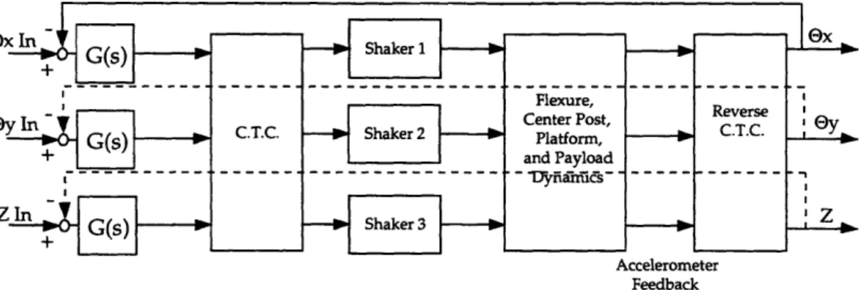
A block diagram of the system appears in Figure 1-3. The three independent

shakers are controlled by the I*star computer, which allows the user to input a power spectral density (PSD) curve of the desired acceleration over the disturbance fre-quency range in each degree of freedom. I*star is capable of generating control spec-tra for three independent axes to yield desired output power specspec-tral densities. This

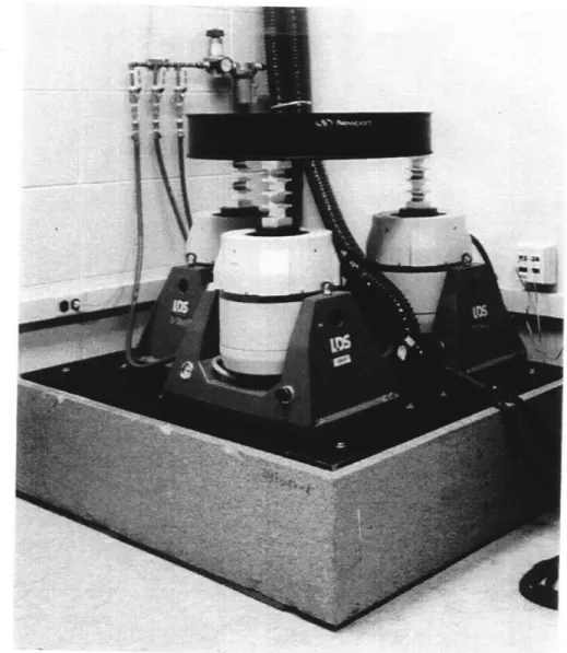
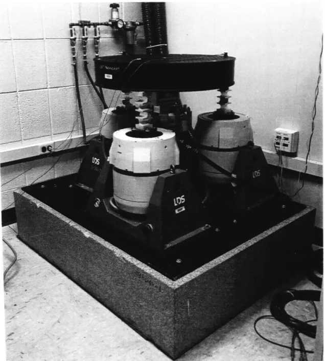
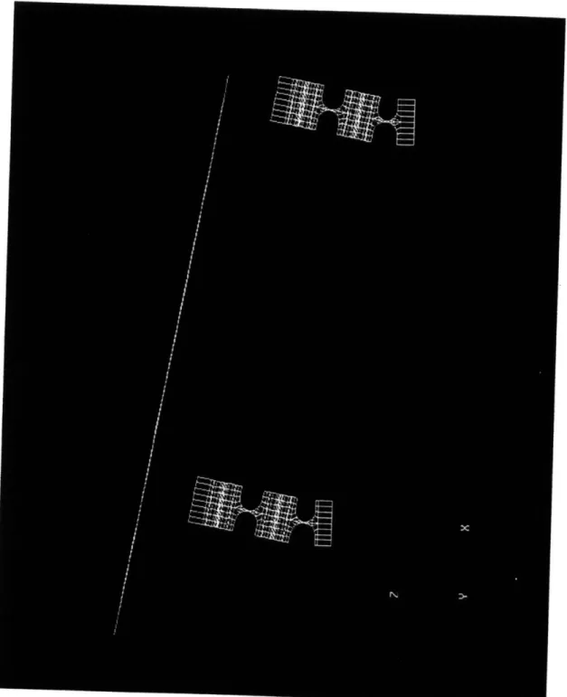
Figure 1-2: Photograph Depicting Shaker Configuration

flexibility allows the ACCEL system to create a wide variety of disturbance environ-ments. The I*star computer also acts as a frequency domain controller; it performs a plant inversion to achieve the desired PSD disturbance levels. It calculates the correct input to the system by inverting the plant transfer function which is in memory and multiplying it by the desired output, specified by the user.

The I*star computer creates control signals in the disturbance axes (08, Os,, and Z). Since the disturbance axes do not match the shaker axes, a coordinate transfor-mation is necessary to convert a command from the former axes to the latter. This

coordinate transformation was developed by Ramona Tung of the Control Systems Engineering Group at Lincoln Laboratory. It basically multiplies the three inputs by a 3X3 transformation matrix utilizing analog circuitry. The outputs from the coordi-nate transformation are then fed to the power amplifiers and then to the actuators. The actuators provide the desired disturbance accelerations to the controlled plant, the payload.

The test payload is mounted to a platform which is attached to the three shakers using three mechanical flexure mounts. These flexures allow the platform to rotate in 0, and 0,. A center post with another flexure system couples the center of the platform to ground in order to restrain the remaining three degrees-of-freedom.

Three accelerometers, one mounted above each shaker, provide the feedback for the system. These signals, however, are in the shaker force axes. Consequently, a reverse coordinate transformation is performed in order to observe the response of the system in the three disturbance axes. This reverse coordinate transformation is the inverse of the previous coordinate transformation matrix. These signals are sent back to the I*star computer as feedback to update the plant transfer function in memory. Control laws to be tested using ACCEL can be defined in the familiar Mat-lab/Simulab programming environment in either state-space or block diagram form. The completed design can then be compiled into executable SPROC code and down-loaded to the chip's memory. The SPROCboard, which houses the SPROC chip, allows the chip to interface with the plant being tested. The performance of the control system can then be evaluated. Alterations to the control system can be per-formed quickly in Matlab and downloaded to the SPROC chip. This portion of the test facility was not developed within the scope of this thesis project.

1.3

_{Performance Specifications of Test Facility}

The performance of the control test facility can be measured by several factors. The system bandwidth, disturbance rejection, stability, maximum angular deflection, max-imum angular and linear acceleration, and maxmax-imum payload mass represent the

2 1

r iControl

in

Coordinate

Figure 1-3: Block Diagram of ACCEL

most important of these factors. Table 1.1 summarizes the performance goals for this project. The maximum accelerations listed are based on bare-table calculations.

Table 1.1: Performace Specifications of Project

Parameter Units Value

Frequency Operation Range Hz 10 to 100

Max Angular Displacement (8, & Oy) mrad ±11.8

Max Linear Displacement inches ±.125

Max Payload weight lb 100

Max Angular Acceleration, 0, rad/sec' 241.3

Max Angular Acceleration, 8, rad/sec2 _278.7

Chapter 2

Literature Review

This chapter outlines prior research projects which were helpful in the development of the three degree-of-freedom vibration test facility. This research includes two beam steering mirror projects developed at Lincoln Laboratory, and a three degree-of-freedom vibration test facility developed for the Syminex Company.

2.1

Beam Steering Mirror Projects

Much of the research performed on beam steering mirrors is applicable to the devel-opment of this test facility. The two projects discussed involve mirrors which, like the mounting platform in this project, can rotate in two degrees-of-freedom. In the case of the steering mirrors, the controlled output are angular positions, whereas angular and linear accelerations are the controlled outputs for the vibration test facility. Two distinct approaches will be evident in the following projects. The large aperture mir-ror incorporates critical damping to allow operation through the undesired modes, leaving the natural frequency unchanged. The small aperture mirror utilizes stiffeners which raise the natural frequencies of the undesired modes well above the closed loop bandwidth, as well as employing damping for part of the system.

Large Steering Mirror

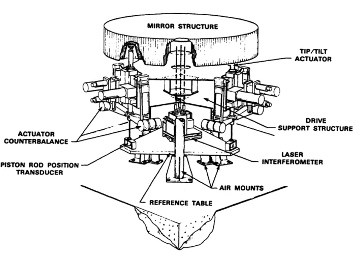
In an effort to demonstrate the feasibility of producing a high performance steering mirror in the 2-4m class, Lincoln Laboratory developed a 2m aperture steering mirror

ACTUATOR COUNTERBALANCE

PISTON ROD POSITIC TRANSDUCER

Figure 2-1: 2m Aperture Beam Steering Mirror

[3]. This mirror consists of an 85 inch diameter by 14 inch deep aluminum honeycomb

sandwich fabricated by Parsons of California. Upon delivery, the structure weighed

300 lb and possessed a freely supported natural frequency of 334 Hz. The mirror was

designed to rotate in two degrees-of-freedom with a maximum angular displacement of ±7.5 degrees. It is supported and driven by three hydraulic actuators spaced 120 degrees apart as shown in Figure 2-1.

The general approach for this project involves critically damping the undesired lateral mode of the mirror system. The actuators are coupled to the mirror using flexible strut dampers and ball joints set into conical frustrum inserts to ensure the center of each ball is located at the transverse center of the structure. Figure 2-2 depicts the strut damper arrangement.

SPRING WASHER UPPER SEAL SPHERE HOUSING LOWER SEAL LOW ROD IT HYDRAULIC CYLINDER TON

Figure 2-2: Flexible Piston for Beam Steering Mirror

STRUT I

The strut damper is a viscous damper acting horizontally between the strut and the hollow piston rods. This damper provides near critical damping to a low natural frequency: a lightly damped lateral rigid body mode of the mirror structure on the struts. The damping forces are obtained from the shearing action of a 0.15 mm thick film of silicone fluid of 600,000 cst viscosity. The shearing action occurs when the mirror rotates through an angle, forcing the struts to sway laterally.

High Bandwidth Steering Mirror (HBSM)

In an effort to produce a small-aperture two axis steering mirror with a closed loop bandwidth of 10 KHz, the HBSM project was developed by Gregory Loney at Lincoln Laboratory [6]. The mirror aperture is only 18 mm with maximum angular displacements of only 20 mrad. The mirror is driven by four magnetic voice coil actuators. Figure 2-3 shows an exploded view of the HBSM design.

Much of the design work focused upon constraining the mirror to prevent motion of the mirror axially, laterally, and torsionally. The degrees-of-freedom which are not actuated were stiffened using an axial flexure and a flexure ring. The system was stiffened to raise the natural frequencies of the modes which couple into the desired mirror motions. The bipod legs of the flexure ring are long low section modulus reed offering little bending stiffness and high axial stiffness. The flexure ring constrains motion coplanar to the mirror and allows rotational compliance about an axis per-pendicular to the mirror normal. This bipod design also resists torsion about the long axis of the axial flexure. The vibrational modes of the bipod legs which compose the flexure ring were additionally damped with a layer of viscoelastic material in order to reduce the coupling between the bipod leg modes and mirror rotation.

This approach was successful in achieving a 10 KHz closed-loop bandwidth, with no significant coupling modes below 20 KHz (the coupling modes of the bipod legs which appear below 10 KHz were well damped).

MAIN HOUSING SENSOR ASSEMBL ACTUATOR - BASE SUPPORT PLATE MIRROR SENSOR PLATE ASSY CLAMP RING RISER SENSOR ELECTRONICS

Figure 2-3: Exploded View of HBSM

END MOT CONNE -RIVETED EAF Y IE

2.2

Syminex Three Degree-of-Freedom Shaker

Sys-tem

A three degree-of-freedom vibration test facility has been developed by Christophe

Touzeau and Stephan Antalovsky for Syminex [14]. The test facility aided in develop-ing a helicopter-borne weapon system involvdevelop-ing an optical sight fixed on a supportdevelop-ing mast above the rotor. The test facility has been designed to accelerate a payload of up to 300 lbs at distinct frequencies which represent the harmonics of the helicopter motion below 100 Hz, as well as provide random noise in the 100-200 Hz frequency range. The vibration environment includes:

1. Two orthogonal rotations at w, nw, and 2nw, maximum ±5.1 degrees

2. Vertical translation at nw

where w is the angular speed of the rotor, and n is the number of blades of the helicopter.

A diagram of the test facility which incorporates three electrodynamic, water-cooled shakers from Ling Dynamic Systems (LDS Model 954LS) is shown in Figure 2-4. The baseplate is accelerated in two orthogonal angular degrees-of-freedom, pitch and roll, and in one linear degree-of-freedom, Z. Feedback was accomplished using one linear accelerometer for Z and two angular accelerometers for the pitch and roll.

The shakers are coupled to a triangular baseplate using three hydrostatic double ball joints. Double ball joints must be used in order to allow the baseplate to rotate through an angle (single ball joints would over-constrain the system). The payload to be tested is mounted to the tip of a mast which is attached rigidly to the baseplate.

The first tests conducted in January 1992 successfully reproduced a number of flight conditions, showing the capability of the system to correctly simulate the com-plex real vibration environment. The control accuracy and repeatability of the proved to be good, with typical accuracies of ±0.2 dB on amplitudes, ±1 degree on phases and ±1l degree on directions of movement [14].

The system performance, however, was limited by the heavily loaded parts, the ball-and-socket bearings and the roller bearing guides, used to allow the fixture to

VERTIC

BEARIN

OAD DISCHARGER

Figure 2-4: Diagram of Syminex 3 DOF Shaker System

TESTED ITEM SUPPORTING MAST BASEPLATE BALL-AND-SOCKET JOINT HYDROSTATIC &OUBLE BALL JOINT ELECTRODYNAMIC EXCITER /: L

rotate and translate. Undesired sine tones which produced errors in payload motion were detected. These problems were the result of the nonlinear behavior of the fixture, and particularly its bearing elements. [2].

Consequently, the development of the vibration test facility at Lincoln Laboratory sought to avoid a bearing system such as the one utilized in the Syminex project, thus circumventing the nonlinearities which are introduced into the system performance.

2.3

Laser Line-of-Sight Control

Jeffrey Ludwig of the Control Systems Engineering Group at Lincoln Laboratory developed a control system to stabilize a space-based laser communications system [7]. A beam steering mirror mounted to a platform was used to focus a laser beam on a detector. The control system was necessary to keep the beam fixed on the detector despite the presence of platform disturbances in one angular degree-of-freedom in a frequency range of 0-50 Hz. The platform disturbances in this project were applied

using one electrodynamic shaker in an arrangement shown in Figure 2-5

The project attempted to constrain the platform motion to pure rotation about one axis. Three identical right angle flexures hinges were designed to accomplish this

goal. One hinge couples the platform to the disturbance actuator, while the other two serve to establish a fixed pivot point directly under the mirror. A sketch of the right angle flexure is shown in Figure 2-6

These flexure hinges possess a low rotational stiffness about one axis, but retain relatively high stiffnesses in the five other degrees-of-freedom. More importantly, the flexures do not introduce nonlinearities into the system; they act as pure torsional springs within their elastic range. This represents a significant improvement over an alternative bearing configuration.

The success of this configuration was limited by the mounting posts which ideally should serve as a fixed point of attachment for two right-angle flexures. These posts in reality act as cantilever beams and allow the platform to displace vertically, as well as rotate. The first structural resonance of these mounting posts appeared at

Beam steering mirror

Inc(

Optical detector

Platform disturbancei

Figure 2-5: Diagram of Single Degree-of-Freedom Line-of-Sight Experiment

approximately 20 Hz. This vertical motion produced an equivalent error observed on the quad cell detector, causing the measured disturbance rejection of the system to be higher in the area of the post resonances.

The research presented was extremely useful in the development of the test facility. This research allowed me to focus upon the areas of design which would be most crucial to successful completion of the project. The following chapter introduces these critical issues as they relate to the vibration test facility.

Chapter 3

Fundamental Issues

This chapter serves as an introduction to the fundamental issues faced during the development of the controls test facility. The dynamics of a six degree-of-freedom model are examined. The dynamics discussion leads to a section which treats the problems of vibrational modes which couple into the actuated degrees-of-freedom of the system. Finally, several basic control issues are discussed.

3.1

Six Degree-of-Freedom Model

An examination of the dynamics of a six degree-of-freedom model aids in predicting the vibrational performance of the system. The purpose of these calculations is to determine the approximate mode shapes for the system. This model will demonstrate that the eigenvectors exhibit coupled motion between several degrees-of-freedom.

Figure 3-1 depicts the model evaluated. Several views are shown in this figure in order to clearly depict the location of the springs attached to the mounting platform. The model consists of the mounting platform, which has a mass m, rotational inertia J in 0, and 0,, and rotational inertia J' in 0~. Translational stiffnesses in X, Y, and Z, and rotational stiffnesses in 0,, 08, and ~, represent the mechanical structures (the flexures and center post) which offer stiffness to the vibrational platform. The model is evaluated with the following assumptions:

b. The platform experiences small angular motion

c. The dynamic effect of the payload is negligible

The platform is not completely rigid at frequencies above 600 Hz, however, this model is developed to study resonances below this frequency. Also, while the payload will greatly influence the dynamics of the system, this model is intended to determine the dynamic behavior of the unloaded system.

Ox

Figure 3-1 a. Mounting Platform Figure 3-1 b. X-Y Plane View of Model

Kz

h h

Ky

Figure 3-1 c. X-Z Plane View of Model Figure 3-1 d. Y-Z Plane View of Model

Figure 3-1: Six Degree-of-Freedom Model

The generalized coordinates for the platform in the model consist of the three

degrees-of-freedom, X, Y, and 8,.

C

= X, Y, Z, ,

0,, OZ

(3.1)

The equations of motion are determined using the Lagrangian approach. The terms for the kinetic energy, T*, and the potential energy, V are:

1 1 2 1 1

j

T* = mi + -m•

+

2

2

2

2

2

2

(3.2)

1 1 1 1 1 1

V= 2kZz+2

k,(x+ h

- rOz)2 2ky(y-hO,

-

2) +2ke,

+

2e+2keO

(3.3)

The Lagrangian is

(3.4)

Lagrange's equations are

i=loi=6

ac

=

EA i =

1

to i = 6,

where E. is the generalized take the following form:

I

+

where [M] is the 6X6 mass stiffness matrix, {x} is the nates, and {F} is the 6X1

force. The resulting equations of motion for the system

C1

K

F ,

matrix, [C] is the 6X6 damping matrix, [K] is the 6X6 6X1 column vector representing the generalized coordi-column vector representing the generalized forces. The damping of the system is small and can therefore be neglected in order to simplify calculations. The mass and stiffness matrices are as follows:

d 0L

and

K1

-kyh

-kh

ke, + kyh

kyhr

+

In order to determine the eigenvectors for the system, we first assume that the solutions to the differential equations take the form:

{((t)} =

and thus

{1(t)} = -W 2

Substituting this into the above equations of

K -

w

_M

eiwt

In order to calculate the natural frequencies and mode shapes, {F} is set to

0. The determinant of the above matrix gives the undamped natural frequencies of

the system. The corresponding mode shapes can be determined by plugging in the natural frequencies and solving for the six column vectors, {vi} which satisfy the

above equation when {F} = 0.

The most important conclusion drawn from this model concerns the form of the eigenvectors. Several of the eigenvectors for the system are coupled between several degrees-of-freedom. The eigenvectors for the system are shown below. The asterisks represent nonzero terms of the vectors.

V1 = * V2 = * * V3 V4 * V5 = * V6 * * * * *

motion in desired and undesired degrees-of-freedom. The three actuators control 0,,

0,, and Z. Motions in X, Y, and 0. are observable but uncontrollable. Consequently,

any mode shape which involves motion in the undesired degrees-of-freedom will be uncontrolled. For example, at the first resonance of the model, the table will be translating in X, and rotating in O6, and #z, but will only be controlled in 0y. The undesired motion in X and 0, presents a serious problem. The coupling in the eigen-vectors cannot be avoided, so the approach followed basically involves maximizing the stiffnesses of the system in X, Y, and 0Z in order to raise the resonances above the desired frequency range of operation. This topic is covered in depth in Chapter

4.

The model also yields the 6X6 transfer function matrix:

K

-

w

_M

_X

Premultiplying by the inverse of the previous matrix yields:

=j K

- w2M

F

= H

F ,

where

H-f₁ Hly f, Hf,. Hxfe Hfze

H yf. Hyfy HB, HI-A,, Hyf H z

Hzf. H.

H

Hzfz

Hzf,.

Hzf

Hzf,,

Hef. Hexfy He.f1 Hxf9x Heo,.y Heyf.s Hoyfx He, , Ho yf. Hoe,6 , Heyfoy Hoyfez

Hezfx Hezfy He•f, Hozfex Hezfey Hozfez

*c *

*c * *

*c

* * *

*i~ * *~i

Each element in the matrix H represents the single-input single-output transfer

tion between the output displacement of the first subscript and the input force of the second subscript. Notice that several of the terms are zero; the elements in boldface and the asterisks again represent the nonzero terms of the matrix.

3.2

Vibrational Coupling

As the block diagram in Figure 1-3 shows, there are two distinct control loops. The user defined control loop which employs the SPROC processing chip, and the control loop about the shaker system which includes the I'star computer. The control system design that will be discussed refers to the latter system composed of the three shakers, the vibrational platform, the flexure mounts and the other mechanical structures attached to the system. In essence, this project is concerned with applying the desired vibrational disturbance to the payload.

The system has a built-in frequency domain controller, the I*star computer, which performs a plant inversion to achieve the desired disturbance. A low-level random noise signal is applied to the system as a pretest and the response is measured in

0,,0,, and Z. Three transfer functions are then calculated: Hdfe , Hefey, and Hif,.

Using the desired output and the transfer function, the I*star controller computes a suitable input to the system. The I*star has two important design performance characteristics. First, it represents an open-loop feed-forward control design; it is not a traditional closed loop system. Secondly, it controls three single-input single output systems; it considers the three actuated degrees-of-freedom as completely uncoupled systems.

Additional time-domain control may be necessary in order to compensate for the coupling which can result from two different sources: coupling between the actuated degrees-of-freedom and coupling caused by the mechanical components of the system. The following sections will elaborate on these sources of coupling.

3.2.1

Coupling Between Actuated Degrees-of-Freedom

The first source of coupling exists between the three actuated degrees-of-freedom for example, driving the system in 0, will result in small motion in 0,. The previous model demonstrates that the actuated degrees-of-freedom are not coupled, but coupling will exist due to imperfections in the mechanical components of the system or small errors in the coordinate transformation circuit. Consider the 6X6 matrix of transfer functions developed in the previous section:

x z OY O, 62

Hxfx

0

0

0

Hx f r

Hx fz

0 Hyfy 0 Hyf _x 0 HyI9 z

0

0

Hzfz

0

0

0

O

Hex f

0

Hexfx

0

Hex fez

Heyfx 0 0 0 Hoyfey Ho fez

Heazx

Ho•

f

0

Hoeziox

He•.oZ

Hezofe

Fx

F

Fz

Fe.

F

_,

Fe.

Now examine the smaller 3X3 matrix of transfer functions which includes only the actuated degrees-of-freedom:

i

HOf- H

f,.

H;f,

Fz,

S Ho-, Ho, - H fy Fa,

The I*star controller treats the actuated degrees-of-freedom as three independent single-input single-output systems. It calculates only the three transfer functions (the diagonals of the matrix). The off-diagonal terms are nonexistent, according to the model. These off-diagonal terms which represent coupling between the actuated degrees-of-freedom, however, may be significant. Since the I*star computes a transfer function between the input of one degree-of-freedom and the output from the same degree-of-freedom, eg. H-fex, any coupling causes the output to be changed. The

I*star computer will sense this coupling, but it will appear as 'artificial resonances' in the three transfer functions. Take, for example, the coupling between 0, and 0,. This

coupling will be observed by the I*star computer, but it will attribute the output motion to only the 8, input. The correct transfer function will not be calculated in this case.

3.2.2

Coupling Caused by Mechanical Components of

Sys-tem

The second source of coupling is a result of the vibrational characteristics of the me-chanical components of the system. The meme-chanical components, such as the flexures and the mounting platform, have their own vibrational modes which change the vi-brational characteristics of the entire system. The previous model shows that the system has mode shapes which exhibit motion in both desired (08, O,, and Z) and

undesired (0z, X, and Y) degrees-of-freedom. Motions in X, Y, and 0. will couple into the three actuated degrees of freedom. The extent to which these motions will couple into the desired degrees-of-freedom depends on the design of these mechanical com-ponents. These components are the main limitation to high bandwidth performance. Consequently, the most in-depth research and testing focused upon the mechanical components of the system: the flexures and the center post.

3.3

Control Issues

Several approaches can be taken to deal with the control aspect of this design problem, but it is important to note that the success of any control system used in the test facility is severely limited by the mechanical design. There are three areas of possible solutions to the problem:

Without the I*star computer in the loop:

a. closing three single-input single-output loops about each actuated degree-of-freedom

With the I*star computer in the loop:

b. utilizing an additional decentralized control which involves input single-output loops about each shaker

c. running the system with the I*star computer as the only controller

It is important to note that depending upon the performance of the open-loop system, a feedback control system may not be beneficial. The system is open-loop stable, so a control system is not necessarily required. However, achieving stability is not a sufficient design goal for a control system. Three other important design factors include stability robustness, and noise and disturbance rejection.

The final choice for the system controller consisted of the I'star computer as the sole controller. This controller was shown to produce adequate results.

3.3.1

Three Single-Input Single-Output Loops About Each

DOF

The coupling resonances introduced by the mechanical components of the system severely limit high bandwidth performance. These coupling resonances are difficult to compensate by electronic means, as described in the HBSM research [6]. By way of illustration, examine the magnitude and phase plots of an ideal transfer function (ratio of acceleration output and voltage input) shown below in Figure 3-2.

This transfer function was chosen to resemble the transfer function of a single degree-of-freedom of the actual system. The system consists of two zeros and four poles. The first critically damped resonance at 20 Hz drops the phase from -180

degrees to -360 degrees (the simulation has offset the phase by -360 degrees). The second underdamped resonance at 600 Hz drops the phase an additional 180 degrees. This ideal system exhibits no coupling resonances; there is a -40 dB/dec rolloff after the second pair of poles.

The general closed loop feedback system block diagram containing disturbance is shown in Figure 3-3 [12]. The system has three inputs: r(s), the command or reference input, d(s), the disturbance, and n(s), the measurement noise which is introduced via sensors. The sensor noise can usually be modeled as uniformly distributed in frequency (white noise). The output of the closed loop system is:

m a, C €-CU "O Frequency in rad/sec U) 0, (I) a. ·t. 100 101 10 103 104 Frequency in rad/sec

Figure 3-2: Ideal Transfer Function

KG(s) 1 KG(s)

y(s) = (s) r(s) + d(s) KG(s) n(s). (3.6)

1 + KG(s) 1 + KG(s) 1 + KG(s)

Since the system is open-loop stable, the main goal of a feedback control system in this case is to enhance the system with disturbance and noise rejection properties.

The second term in the above equation represents the disturbance effect in the system. In order to reduce the effect of d(s), the loop gain KG(s) must be kept large in regions where d(s) is large. Assuming that the disturbances will be low frequency, the controller will be designed to raise the loop gain in the low frequency range of the open loop transfer function. The block diagram for this controller is shown in Figure 3-4. There are three single-input single-output loops about each degree-of-freedom.

+ y

Figure 3-3: General Closed Loop Block Diagram Including Disturbance and Measure-ment Noise Inputs

rejection abilities because its loop gain rolls off at low frequencies. Consequently, the low frequency response of the system must be altered. Two lag compensators are added to the system (two poles at .159 Hz and two zeros at 10 Hz), along with an integrator at .159Hz. This raises the loop gain at low frequencies, thus attenuating d(s). The lag compensator, however, does produce a phase drop in the system, but this drop is far enough removed from the crossover frequency to not affect the stability of the system.

The third term in the above equation represents the noise effect in the system. In order to suppress the noise, the loop gain must be kept small in regions where n(s) is large and tight command-following is not required. Thus, the compensated system should roll off at high frequencies. The pure integrator term ensures that the system will sufficiently attenuate high frequency noise by decreasing the slope of the transfer function.

Finally, a gain is chosen to produce the desired crossover frequency of 200 Hz. The compensated system has a phase margin of 59.0 degrees. The compensation design process followed is outlined [Roberge]. The block diagram of the compensated system is shown in Figure 3-5 and the compensated open-loop transfer function is shown in Figure 3-6.

ex

In

ey

K

EOy

Figure 3-4: Closed Loop Block Diagram of Single-Input Single-Output Control Scheme

In reality, however, the transfer functions exhibit coupling modes which appear as spikes in the phase and magnitude plots. This problem was encountered in the HBSM project [6]. These coupling modes limit the bandwidth of the system. As the bandwidth of the system increases, these modes cause the servo loop to become unstable. The resonances appear as spikes in magnitude and phase at frequencies above the crossover frequency. If these resonances are not attenuated properly, they may push the magnitude above 0 dB, causing instability. To ensure stability, the first coupling resonance must be roughly a factor of 4 greater than the cross over frequency. There is a tradeoff between stability and disturbance rejection on one hand, and bandwidth on the other.

The same system, however, operated open-loop without compensation has a much greater bandwidth, retains stability (since the system is open-loop stable), but does not possess any enhanced disturbance or noise rejection properties. The open-loop system can be operated at a frequency just below the first coupling resonance, thus increasing the frequency operation range.

In conclusion, feedback would unnecessarily limit the bandwidth of the compen-sated system if the transfer functions are well-behaved. In this case, the I*star con-troller will provide sufficient control. The system transfer functions are well-behaved if they are stable, smooth, and show no coupling between actuated degrees-of-freedom

Controller I I I I I I L,-I I I I I I I 1 I 1 I II s2+251s+15791 1 -ls2+7540s+7.10E6 f I I I I I I I Mant

Figure 3-5: Compensated Closed Loop Block Diagram

over the desired frequency range. Strangely enough, a feedback control system may not improve system performance.

3.3.2

I*star Controller Alone

The I*star controller represents a feed-forward controller which utilizes estimates of the plant transfer function in order to shape the input to achieve the desired output. Figure 3-7 shows a block diagram of the control system.

A closed-loop feedback controller is not required because the system is open-loop

stable, but it would provide the system with disturbance rejection which the I*star controller cannot. The I*star controller, using plant inversion, does not perform well near undamped resonances or in regions which exhibit the first form of coupling men-tioned: coupling between actuated degrees of freedom. However, the I*star performs well in other areas. It has the benefit of allowing the system to be operated at higher frequencies than a closed loop system.

I I I I

C a) IC~ 0) Cu 100 101 102 103 104 Frequency in rad/sec zuu a) a) o -200 40 _AL t 100 101 102 103 104 Frequency in rad/sec

Figure 3-6: Compensated Ideal Transfer Function

3.3.3

Three Single-Input Single-Output Loops About Each

Shaker

Three single-input single-output loops about each shaker could be utilized in addition to the I*star controller to give the system disturbance and noise rejection properties, as the single loops about each degree-of-freedom could but without sacrificing band-width. A block diagram for this control scheme is shown in Figure 3-8.

The benefit of placing the control loops about the shakers lies in a larger possible bandwidth. The feedback for the control loop would be provided by an additional set of accelerometers, one directly on the mounting plate of each shaker. The goal of this approach is to control a transfer function which has resonances which are of lower frequencies than those of the entire flexure/platform system. For example, the

43

; :; I : ;: I I :;

Istar Estimate H

of Transfer Functions Accelerometer

Feedback

-11

(x

Ox In

()x

Desired ax

Flexure,

)y

In

Center Post,

Reverse

Desired Ey and Payload

Dynamics

Z

ZI

I

H

Desir HZ Shaker 3

--- I

Figure 3-7: I*star Controller Block Diagram

Signals H' from Istar rix In Oy In Z In ----C.T.C. G (s) Shaker 1 Flexure,

Center Post, Reverse

G(s) Shaker 2 Platform, - - C.T.C. and Payload Dynamics G(S) Shaker3 I+!

OX

ey

z

Figure 3-8: Three SISO Loops About Each Shaker

flexure/platform system will exhibit natural frequencies below 600 Hz, but the shakers

are limited by the resonance of the armature which occurs at 4850 Hz. The placement

of the accelerometers attempts to ensure the resonances introduced by the flexures and the mounting platform will not appear in the controlled transfer function. This allows the cross over frequency of the controlled system to be placed higher than the previous single-input single-output design, while still giving the system disturbance

and noise rejection properties.

This approach is limited by the influence of the dynamics of the flexures and platform. A simple two degree-of-freedom model shown in Figure 3-9 illustrates this

point. The mass mx represents the armature of a single shaker, kI the axial stiffness of a single shaker, c2 the damping of the flexures, m2 the mass of the platform, and

k2 the stiffness of the flexures.

A

TX

2

2

Figure 3-9: Two Degree-of-Freedom Model

The transfer function relating the displacement of mi to an input force, F1, applied

to mr is:

(k2 + m2s2) + sc2

[(kl + mis2)(k2+ m2s2) + m2k2s2] + scz [(ml + m2)s2 + k-2]

(3.7)

The acceleration of the armature is dependent upon the dynamics of the flex-ure/platform combination. Consequently, the success of this approach relies upon attenuating the effect of the dynamics of the flexures/platform combination.

Chapter 4

Component Characterization and

Design

In this chapter, the main components of the three-degree-of-freedom vibration test fa-cility are described, along with the performance specifications which drove the design. The performance of the components is judged primarily upon their frequency response characteristics. The vibrational behavior of mechanical components, in particular, the location of the natural frequencies introduced by the components is examined closely. The components discussed in this chapter include the coordinate transformation circuit, the electrodynamic shakers, the vibrational mounting platform, the four-axis flexures, the center post, and the accelerometers used to provide feedback for the system.

4.1

Coordinate Transformation Circuit

The coordinate transformation circuit was developed and built by Ramona Tung of

the Control Systems Engineering Group at Lincoln Laboratory. This circuit trans-forms the disturbance axes (0,, 0,, and Z) into the shaker axes (1, 2, and 3) by

converting the desired rotation and translation into three linear motions with differ-ent phases. The force axes of the three shakers do not align with the disturbance axes

required to allow the user to create a vibrational environment using the disturbance axes. The feedback for the system is accomplished through the use of three linear ac-celerometers positioned on the vibrational platform directly above each shaker. These signals are aligned with the force axes of the shakers, so a reverse coordinate trans-formation is necessary to feed back the correct signals. This reverse transtrans-formation matrix is the inverse of the transformation matrix. By assuming the disturbance axes are aligned with the principal axes, the center of gravity of the assembly is at the geometric center of the platform, and that the platform is perfectly rigid, the 3X3 matrix which relates the actuator axes and the disturbance axes is easily derived from geometry and rigid body mechanics [15]. See Appendix A for discussion. The transformation matrix is shown below:

e

g,

0.264

0.152 1.0

Ox

=

M

e8

Z

Z

0.0

-0.305 1.0

2

Where the column vector composed of Z1, 2, and Z3 represents the control inputs in

the shaker force axes, and the column vector composed of §,, 8~ and 2 represents the control inputs in the disturbance axes. Again, the reverse coordinate transformation, which converts the accelerometer outputs in the shaker axes to the disturbance axes is simply the inverse of the transformation matrix, M-l:

8, ZI 1.894 -1.894 0.0 zi

S= M- 1 2 = 1.094 1.094 -2.187 22 (4.2)

Z Z3 0.333 0.333 0.333 Z3

where the column vector composed of Z1, Z2, and 3 s represents the accelerometer

outputs in the shaker force axes, and the column vector composed of J8, 8, and 2 represents the accelerometer output in the disturbance axes.

4.2

Electrodynamic Shakers

The electrodynamic shakers used in the test facility are model V556 purchased from Ling Dynamic Systems. The theory of operation is very simple. Each shaker houses a wire coil which is attached to the moving element of the shaker, the armature. A magnetic field is produced by an electromagnet within each shaker. When current is applied to the coil in the magnetic field, a force F proportional to the current I and the magnetic flux intensity B, is produced which accelerates a component mounted to the surface plate of the shaker:

F = BIl (4.3)

where 1 is the length of coil. By applying a sinusoidal current to the shaker, the armature translates vertically, thus accelerating the payload in one linear degree-of-freedom. The current is supplied to the shaker by a power amplifier which converts an input voltage to an output current. The armature features a light weight, rugged magnesium frame which ensures a high natural frequency. In order to ensure linear motion of the armature, each shaker is equipped with a suspension system. A cross-section of one of the electrodynamic shakers used in the test facility is shown in Figure 4-1.

Table 4.1 describes the various performance characteristics of each shaker [4]. The high cross-axial (lateral) and rotational stiffnesses of the shaker are provided by four low mass suspension rollers running on flexures and a central linear bearing system. The polypropylene flexures attached to the rollers bend as the armature translates vertically. The suspension rollers are preloaded to ensure that no chatter will occur during operation. Two rubber shear mounts also link the armature to the shaker housing. These mounts provide the axial stiffness and, more importantly, damping to the vertical motion of the shaker. The lower guidance system for the armature features a linear ball bearing with nylon balls. The linear bearing is produced by Ransom, Hoffman, and Pollard of England.

Figure 4-1: Cross Section of LDS Model V556 Vibration Generator Table 4.1: Shaker Performance

Parameter Units Value

Frequency Operation Range Hz 5 to 6300

Random Force (rms) lbf 80

First Armature Resonance Hz 4850 Max Payload Weight lbf 55

Max Rated Travel inches

+.50

Axial Stiffness lbf/in 90

Rotational Stiffness lbf/in 72,000