Development and Application of a 4-Dimensional
Computed Tomography Simulator
by
Alan Chu
S.B., Electrical Engineering and Computer Science, Massachusetts
Institute of Technology, 2006
Submitted to the Department of Electrical Engineering and Computer
Science
in partial fulfillment of the requirements for the degree of
Master of Engineering in Electrical Engineering and Computer Science
at the
MASSACHUSETTS INSTITUTE OF TECHNOLOGY
May 2007
c
Massachusetts Institute of Technology 2007. All rights reserved.
Author . . . .
Department of Electrical Engineering and Computer Science
May 25, 2007
Certified by . . . .
George T.Y. Chen
Director, Radiation Physics Division, Department of Radiation
Oncology, Massachusetts General Hospital, Professor of Radiation
Oncology, Harvard Medical School
Thesis Supervisor
Certified by . . . .
William M. Wells
Research Scientist, MIT CSAIL, Associate Professor of Radiology,
Harvard Medical School and Brigham and Women’s Hospital
Thesis Supervisor
Accepted by . . . .
Arthur C. Smith
Chairman, Department Committee on Graduate Theses
Certified by . . . .
Gregory C. Sharp
Radiation Physicist, Department of Radiation Oncology,
Massachusetts General Hospital
Instructor, Harvard Medical School
Thesis Supervisor
Certified by . . . .
John A. Wolfgang
Radiation Physicist, Department of Radiation Oncology,
Massachusetts General Hospital
Instructor, Harvard Medical School
Thesis Supervisor
Development and Application of a 4-Dimensional Computed
Tomography Simulator
by
Alan Chu
Submitted to the Department of Electrical Engineering and Computer Science on May 25, 2007, in partial fulfillment of the
requirements for the degree of
Master of Engineering in Electrical Engineering and Computer Science
Abstract
This thesis presents the development and application of a 4-Dimensional Computed Tomography (4D CT) simulation program. The simulation is used to understand and quantify the sources of image artifacts that arise from irregular patient breathing during 4D CT. Performance of the simulation is validated by comparing the simu-lation results with those of phantom experiments with CT scanners. The program simulates 4D CT scanning of objects of arbitrary size and shape and is extended to investigate the accuracy of gated radiotherapy. Experiments are performed using realistic breathing patterns from patients, in addition to synthetic ones for various studies. The simulation is used to study the effects of scan start time shift, breathing trace baseline drift, and hysteresis of internal organ and abdominal surface motion on the quality of 4D CT images.
While 4D CT significantly reduces artifacts from helical scans of the thoracic and abdominal areas, a variety of different sources can still contribute to motion-induced artifacts in 4D CT. Since 4D CT is used to determine target margins for radiotherapy, proper precaution should be taken so that image artifacts do not lead to inaccurate treatment planning. Finally, this thesis discusses improvements in 4D CT and suggests additional methods to improve treatment planning for radiotherapy. Thesis Supervisor: George T.Y. Chen
Title: Director, Radiation Physics Division, Department of Radiation Oncology, Massachusetts General Hospital, Professor of Radiation Oncology, Harvard Medical School
Thesis Supervisor: William M. Wells
Title: Research Scientist, MIT CSAIL, Associate Professor of Radiology, Harvard Medical School and Brigham and Women’s Hospital
Acknowledgments
First, I would like to thank Dr. George Chen for his support and guidance on this research. He is an extremely busy person, but always finds the time to see his students. It was through his support that I was able to work at Massachusetts General Hospital, and I learned a great deal from him not only about medical physics and imaging, but about graduate research as well.
The contributions of Dr. Sandy Wells were also very helpful for this thesis. I was fortunate enough to take a class taught by him, and I received useful ideas from my experiences there. I thank him for all the edits he made in preparing this thesis.
Dr. Greg Sharp and Dr. John Wolfgang provided a great deal of technical exper-tise in 4D CT. Whenever I was confused about an issue, a conversation with one of them would clear things up dramatically. I thank John for repeatedly answering all my questions. Greg provided a lot of useful code to me, and also provided knowl-edgeable answers to my numerous questions about 4D CT and radiotherapy. I would also like to thank Kit Mui for providing helpful code and the Boston Medical Center for the use of their CT scanner.
Contents
1 Introduction 17
1.1 Brief History of CT Scanning . . . 17
1.2 Motivation . . . 18
1.2.1 Role of 3D Anatomical Imaging in Radiotherapy . . . 18
1.2.2 Problems with 3D CT . . . 19
1.2.3 4D Radiotherapy . . . 20
1.3 Goals and Purposes . . . 20
2 Background and Theory of 4-Dimensional Computed Tomography 21 2.1 Introduction to 4D CT . . . 21
2.1.1 Origins and Purpose of 4D CT . . . 21
2.1.2 Overview of the 4D CT Algorithm . . . 22
2.2 Hardware Configurations . . . 24
2.2.1 Scanners . . . 24
2.2.2 Respiratory Monitors . . . 25
2.3 Reconstruction Approaches . . . 26
2.3.1 General Electric Scanner - Cine Mode . . . 26
2.3.2 Philips Scanner - Sorting in Sinogram Space . . . 27
3 Methods 29 3.1 Experiments . . . 29
3.1.1 General Electric CT Scanner . . . 29
3.1.3 Breathing Traces . . . 31
3.1.4 Breathing Trace Analysis . . . 33
3.1.5 Error Quantification . . . 34
3.2 4D CT Simulations . . . 35
3.2.1 General Electric Scanner Experiment Simulations . . . 35
3.2.2 Comparison of Simulations to Experiments . . . 37
3.2.3 Time Shift Simulations . . . 39
3.2.4 Hysteresis . . . 40
3.2.5 Baseline Drift . . . 41
3.2.6 Arbitrary Object Simulations . . . 43
3.3 Radiation Treatment Simulations . . . 44
4 Results 47 4.1 Breathing Trace Analysis . . . 47
4.2 Experiments . . . 50
4.2.1 General Electric CT Scanner . . . 50
4.2.2 Philips CT Scanner . . . 55
4.2.3 Comparison of General Electric and Philips Scanners . . . 55
4.3 4D CT Simulations . . . 65
4.3.1 Comparison of Simulations to Experiments . . . 65
4.3.2 Time Shift Simulations . . . 67
4.3.3 Hysteresis . . . 69
4.3.4 Baseline Drift . . . 69
4.3.5 Arbitrary Object Simulations . . . 74
4.4 Radiation Treatment Simulations . . . 77
5 Concluding Remarks 81 5.1 Summary . . . 81
5.2 Suggestions and Future Work . . . 84
5.2.1 4D CT Algorithm Improvements . . . 84
5.2.3 Alternative Methods of Quantifying 4D CT Error . . . 87
List of Figures
2-1 Diagram for phase-based 4D CT image reconstruction at the exhale phase. . . 24 3-1 Phantom positioned on the computer-driven sled, which was used in
the 4D CT experiments. . . 30 3-2 Breathing traces 2563 (displayed using a scale factor of 3) and 2567
(displayed using a scale factor of 2). The peaks of the traces correspond to exhale and the valleys correspond to inhale. . . 32 3-3 Diagram for volume computation. . . 37 3-4 Diagram for computation of the acquisition amplitude of the first
four-slice section that four-slices through Sphere 1. . . 39 3-5 Example of baseline drift in a breathing trace. The black trace is the
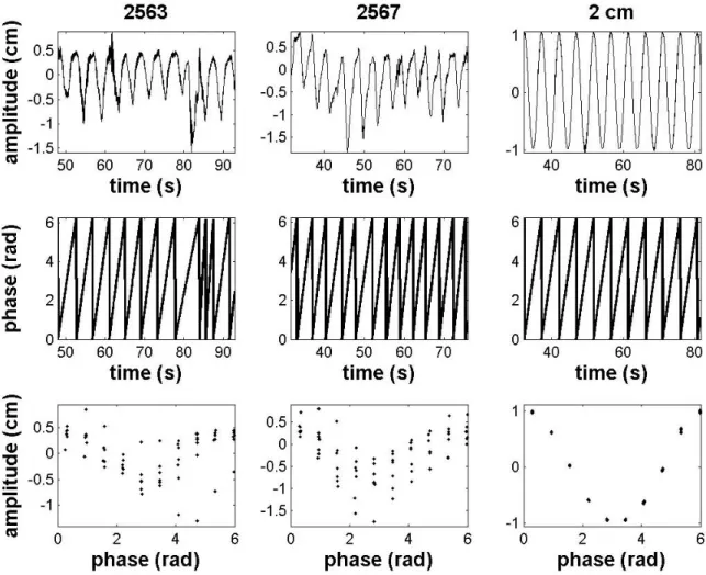
original sinusoidal breathing trace. The red dotted trace has a positive slope, resulting in baseline drift. The orientation of the traces is such that the peaks correspond to exhale, and the valleys correspond to inhale. 42 4-1 Amplitude, phase, and amplitude phase correlation of traces 2563,
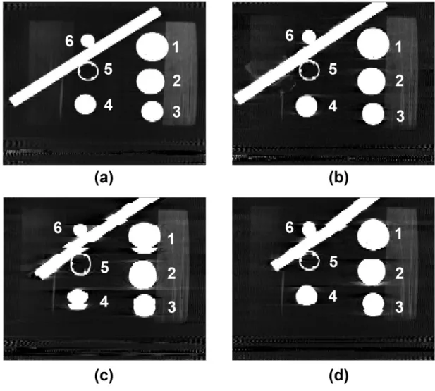
2567, and 2 cm peak to peak sine wave. The segments shown in the figure correspond to segments where Sphere 1 was scanned by the GE scanner. The internal-external motion scale factor is incorporated into the amplitude plots, which correspond to the true motion of the phantom. 48 4-2 Using the GE scanner, (a) coronal slice of static phantom; coronal slice
of phantom at 50% (inhale) phase for (b) 2 cm sine, (c) 2563 trace, (d) 2567 trace. . . 51
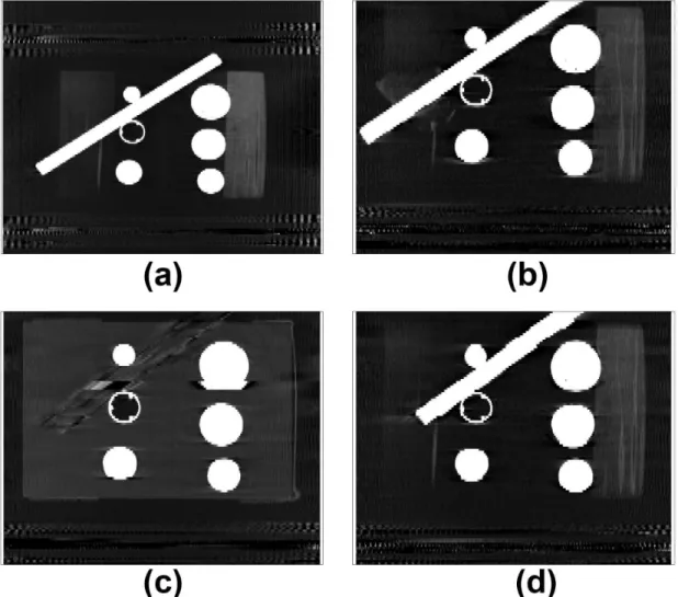
4-3 Using the GE scanner, (a) coronal slice of static phantom; coronal slice of phantom at 0% (exhale) phase for (b) 2 cm sine, (c) 2563 trace, (d) 2567 trace. . . 53 4-4 Volume of Sphere 1 for different traces as a function of respiratory
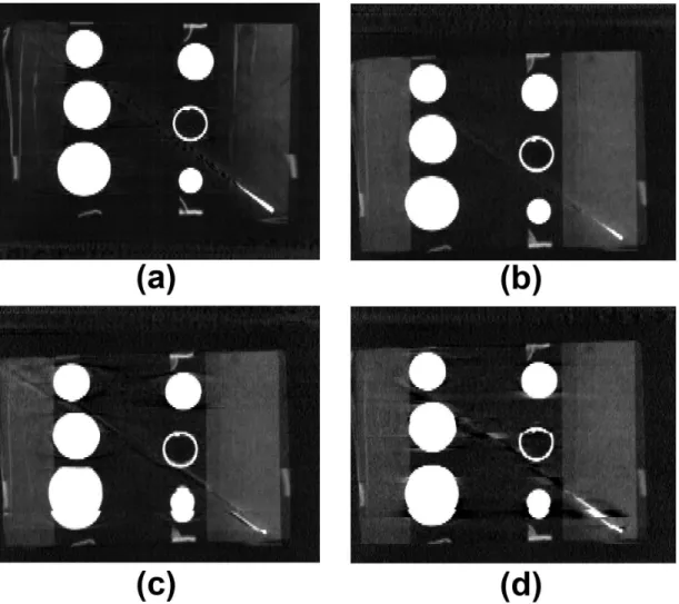
phase using the GE scanner. These volumes were computed using the GE Sim4D tools. . . 54 4-5 Using the Philips scanner, (a) coronal slice of static phantom; coronal
slice of phantom at 0% (inhale) phase for (b) 2 cm sine, (c) 2563 trace, (d) 2567 trace. . . 56 4-6 Using the Philips scanner, (a) coronal slice of static phantom; coronal
slice of phantom at 40% (close-to-exhale) phase for (b) 2 cm sine, and at 50% (exhale) phase for(c) 2563 trace, (d) 2567 trace. . . 57 4-7 Image volume of Sphere 1 using the GE and Philips scanner as a
func-tion of respiratory phase for trace 2563. . . 58 4-8 Image volume of Sphere 1 using the GE and Philips scanner as a
func-tion of respiratory phase for trace 2567. . . 59 4-9 Image volume of Sphere 1 using the GE and Philips scanner as a
func-tion of respiratory phase for 1 cm sine trace. . . 60 4-10 Image volume of Sphere 1 using the GE and Philips scanner as a
func-tion of respiratory phase for 2 cm sine trace. Note that the Philips plot only contains volumes for phases 0%, 10%, 20%, 30%, and 40%. . . . 60 4-11 Z-coordinate of Sphere 1 center of mass using the GE and Philips
scanner as a function of respiratory phase for trace 2563. X-coordinate and y-coordinate are constant throughout all phases. . . 62 4-12 Z-coordinate of Sphere 1 center of mass using the GE and Philips
scanner as a function of respiratory phase for trace 2567. X-coordinate and y-coordinate are constant throughout all phases. . . 63 4-13 Z-coordinate of Sphere 1 center of mass using the GE and Philips
scanner as a function of respiratory phase for 1 cm sine trace. X-coordinate and y-X-coordinate are constant throughout all phases. . . . 63
4-14 Z-coordinate of Sphere 1 center of mass using the GE and Philips scanner as a function of respiratory phase for 2 cm sine trace. X-coordinate and y-X-coordinate are constant throughout all phases. Note that the Philips plot only contains COMs for phases 0%, 10%, 20%, 30%, and 40%. . . 64 4-15 (a) 4D CT simulation image of Sphere 1 using 2563 respiration trace
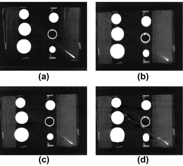
at inhale phase, (b) 2563 amplitude trace, and (c) corresponding phase trace determined by RPM software. Inset (upper left) shows the orig-inal 4D CT reconstruction image of Sphere 1 from the phantom scan. 66 4-16 Time shift 4D CT simulation images of Sphere 1 using 2563 respiration
trace at inhale phase. Results of starting the scan at the (a) sixth couch position, (b) seventh couch position, (c) eleventh couch position, and (d) twelfth couch position. . . 68 4-17 Hysteresis 4D CT simulation images of Sphere 1 using 2563 respiration
trace at inhale phase. Results of using a hysteresis delay of (a) 31 ms, (b) 63 ms, (c) 94 ms, and (d) 125 ms. . . 70 4-18 Hysteresis 4D CT simulation images of Sphere 1 using 2563 respiration
trace at inhale phase. Results of using a hysteresis delay of (a) 156 ms, (b) 188 ms, (c) 219 ms, and (d) 250 ms. . . 71 4-19 Baseline drift 4D CT simulation images of Sphere 1 at inhale using a
2 cm sine wave with a slope of (a) 0 cm/s, (b) 0.0136 cm/s, (c) 0.0268 cm/s, and (d) 0.0400 cm/s. . . 72 4-20 Image volume of Sphere 1 at 50% (inhale) phase as a function of the
baseline drift slope of a 2 cm sine breathing trace. . . 73 4-21 Coronal cut of a 3D static scan of Sphere 1, which is used as input to
our simulation of arbitrary objects. . . 74 4-22 4D CT simulation image of Sphere 1 using 2563 respiration trace at
inhale phase. The input object is the static 3D scan of Sphere 1, shown in Figure 4-21. . . 75
4-23 The left side shows the 4D CT simulation image of Sphere 1 using the 2563 respiration trace at 10% phase. The right side shows the experimental result from the GE scanner at 10% phase. The input object is the static 3D scan of Sphere 1, shown in Figure 4-21. . . 76 4-24 The left side shows the 4D CT simulation image of Sphere 1 using
the 2563 respiration trace at 80% phase. The right side shows the experimental result from the GE scanner at 80% phase. The input object is the static 3D scan of Sphere 1, shown in Figure 4-21. . . 77 4-25 Breathing trace of a patient undergoing gated radiation treatment.
The gating trace is in blue, dotted with red points where treatment commenced. The amplitudes are not scaled by any factor, and an amplitude of 0 is the mean of the entire breathing trace. . . 78 26 Radiation treatment simulation using the breathing trace in Figure
4-25 with the tumor depicted as the smaller circle and the aperture as the larger circle. The square wave denotes when treatment commenced (1 = beam on, 0 = beam off). . . 79
List of Tables
4.1 Characteristics of 122 different breathing traces. No scale factor was used. . . 50 4.2 Image volumes of Sphere 1 in cm3 for the GE and Philips scanners. . 61 4.3 Z-coordinate of image center of mass (COM) of Sphere 1 in centimeters
Chapter 1
Introduction
This thesis presents the development and application of a 4-Dimensional Computed Tomography (4D CT) simulation program. The simulation is used to understand and quantify the sources of image artifacts that arise from irregular patient breathing during 4D CT. Performance of the simulation is validated by comparing the simu-lation results with those of phantom experiments with CT scanners. The program simulates 4D CT scanning of objects of arbitrary size and shape and is extended to investigate the accuracy of gated radiotherapy. Experiments are performed using realistic breathing patterns from patients, in addition to synthetic ones for various studies. The simulation is used to study the effects of scan start time shift, breathing trace baseline drift, and hysteresis of internal organ and abdominal surface motion on the quality of 4D CT images.
1.1
Brief History of CT Scanning
Computed Tomography (CT) technology has greatly improved in image quality and speed since the first scanner was built in 1972 by Godfrey Newbold Hounsfield. The first generation of CT scanners used a single x-ray source, a single detector, and a pencil x-ray beam to acquire a set of parallel projection data for each rotation angle [14][22]. The second generation of CT scanners used multiple detectors and a narrow fan beam, and was more efficient than the first generation. In the first two
generations, the source and detector translated and rotated around the patient to acquire projections for reconstruction.
The third generation of CT scanners used a fan beam and detectors that could measure the projection across an entire cross-section. Therefore, translation across the patient was not needed, and a rotation of both the source and detector was sufficient to capture an image. However, this setup produced many artifacts caused by the loss of calibration in the detectors from rotational motion[22].
The fourth generation of CT scanners used a ring of fixed detectors and a ro-tating source. This arrangement eliminated most of the artifacts due to detector performance. However, fourth generation scanners needed a larger number of detec-tors, which increased the cost of CT scanners. In addition, the fourth generation was more sensitive to scatter radiation.
Helical CT scanning was a further improvement to CT scanners. In helical CT, the couch moves smoothly through the rotating gantry during scanning. In previous generations, the couch was stationary for the acquisition of one slice, after which the couch would move to the next stationary position for the next slice. Helical CT greatly improved the speed of scanning. In addition, many helical scanners have multiple detector rings, allowing the acquisition of multiple slices with each gantry rotation.
1.2
Motivation
1.2.1
Role of 3D Anatomical Imaging in Radiotherapy
3-Dimensional imaging is an important part of radiation treatment planning. Along with physical examination, 3D imaging is used to determine the gross tumor volume (GTV), which includes the gross disease [21]. The GTV is expanded to include areas of high risk of disease into the clinical target volume (CTV). An internal margin is added to the CTV to accommodate organ motion and variations in size and shape of the CTV. This volume is called the internal target volume (ITV). Finally, a setup
margin around the ITV is included to compensate for the uncertainty involved in day-to-day patient setup, resulting in the planning target volume (PTV).
The accuracy of tumor imaging becomes even more important when tumors are located very near critical structures such as the heart, lung, or spinal cord. The overall goal of radiotherapy is to control malignant cells through the use of radiation while at the same time sparing as much of the surrounding tissue as possible. In some situations, the target volume may only be a few millimeters away from a critical structure. Inaccuracies in imaging may result in radiation toxicity to the patient if the target is too large. On the other hand, if the target volume does not adequately cover the diseased tissue, malignant cells may not be entirely irradiated and the disease may spread to surrounding areas.
1.2.2
Problems with 3D CT
Helical CT scanning of thoracic and abdominal tumors can produce significant motion artifacts in both clinical and phantom studies [7][10][23]. These artifacts are mainly generated by respiratory-induced motion of the patient. In addition, image distortions can be introduced by movement of the tumor during a gantry rotation. Since CT images of tumors are used for radiation treatment planning, CT image artifacts can significantly reduce the accuracy of target delineation.
3D CT operates under the assumption that the patient’s anatomy is motionless during scanning, which can lead to respiratory-induced motion artifacts in the CT images. Recently, 4D CT was developed to accommodate the respiratory motion of the patient during scanning.
The clinical use of 4D CT for radiation treatment planning has been increas-ing [2][13]. The increase in 4D CT is due in part to the expectation that 4D CT images of thoracic and abdominal tumors are much more accurate than those pro-duced by 3D CT [8]. However, it is important to examine and quantify the accuracy of 4D CT images using different breathing patterns to see if the images are adequate for clinical use.
1.2.3
4D Radiotherapy
Radiotherapy suffers from respiratory motion induced problems when the tumor is located in the chest or abdominal area. Even if the shape and size of the tumor are known, the accuracy of tumor irradiation decreases because of target respiratory motion. 4-Dimensional radiotherapy seeks to mitigate these problems by tracking the tumor’s location during treatment.
In respiratory-gated radiotherapy, the treatment beam is turned on only when the tumor reaches a specified location. Treatment can also be gated based on respiratory phase; for example, the beam is turned on only at full exhale. This approach allows the design of smaller apertures1 since the apertures do not have to cover the full extent of tumor respiratory motion. In principle, 4D radiotherapy provides accurate irradiation of the tumor while sparing more of the surrounding healthy tissue.
4D CT is especially useful for 4D radiotherapy since 4D CT provides images of the tumor at different phases in the patient’s respiratory cycle. These images allow radiation oncologists to examine the respiratory motion of the tumor and to design an appropriate treatment plan for the patient.
1.3
Goals and Purposes
One objective of this research is to examine the feasibility of using 4D CT images for radiotherapy. In order for target margins to be set accurately, the tumor images used in planning need to be sufficiently truthful. The 4D CT simulation program efficiently produces results without having to physically use the 4D CT scanning equipment. This research takes advantage of the simulation by performing numerous 4D CT studies with varying scan parameters. Finally, this thesis presents ideas on improving 4D CT through the use of simulation and alternative imaging techniques.
Chapter 2
Background and Theory of
4-Dimensional Computed
Tomography
This chapter provides a brief overview of 4-Dimensional Computed Tomography (4D CT) and the different hardware and software components it uses. This chapter starts out by introducing the problems in medical imaging that prompted the invention of 4D CT, and then covers some of the methods currently used in 4D CT.
2.1
Introduction to 4D CT
2.1.1
Origins and Purpose of 4D CT
Respiratory-induced motion of tumors and normal tissues can cause significant arti-facts in images acquired by helical CT scanning [3]. 4D CT was invented as a way to account for the respiratory motion during imaging, and to produce accurate images of a tumor at different phases in the patient’s breathing cycle. 4D CT is an integral step used in 4-Dimensional radiotherapy and has been used as part of the planning process for radiotherapy in clinical settings [1][2][13][16][18].
accurate than ones produced by helical CT [19]. The accuracy of these 4D CT images can increase the accuracy of tumor delineation for radiation treatment.
Another advantage of 4D CT is that it provides information about the locations of the tumor over a period of approximately 2 minutes. In other words, each image is reconstructed from data that was acquired throughout a span of several minutes. Since 4D CT produces images at a number of different phases in the patient’s breath-ing cycle, the images provide information on the “average” trajectory of the tumor for a cycle of breathing.
2.1.2
Overview of the 4D CT Algorithm
4D CT uses information from the real-time monitoring of a patient’s breathing during the scan. This monitoring can be performed using a number of different methods, as described in Section 2.2.2, but the result is a waveform that approximates the anterior-posterior position of the patient’s abdominal surface as a function of time. An assumption is made that this abdominal surface waveform is directly correlated to the cranial-caudal motion of the patient’s internal organs as a function of time. During scanning, the acquisition time of each image slice is recorded so that the slices can be selected based on their acquisition time once the scan is completed. Respiratory phases (0 through 2π) are assigned to each point of the waveform. Phases can also be specified as percentages of the radian phase, such as 0%, 10%, 20%, . . ., 90% of 2π.
4D CT uses a conventional 3D CT scanner coupled with a breathing monitor. In cine mode 4D CT, the couch stops at one of multiple pre-defined couch positions1
while the scanner continuously acquires data. The duration of these stationary couch positions are set for at least one period of the patient’s breathing, which is approx-imately 4 to 5 seconds. The x-ray beam is then turned off and the couch is moved to the next position, where the process repeats. Couch translation limits are set to cover the entire cranial-caudal imaging region of interest (ROI); couch positions do not overlap areas of imaging.
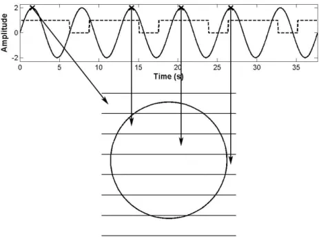
Figure 2-1 shows a diagram that explains the general principles behind phase-based image reconstruction2 in 4D CT. In this figure, the circle represents a coronal
cut3 of the reconstructed image of a sphere. The patient’s breathing trace4 waveform
is shown above the image, along with a square wave indicating when the x-ray beam turns on and off (1 for on, 0 for off). The square wave also indicates the couch positions since the beam is turned on at a couch position, and the beam is turned off while the couch is moved to the next position. The breathing trace is oriented such that exhale corresponds to the peaks and inhale corresponds to the valleys.
The image in Figure 2-1 is reconstructed at the exhale phase. Crosses in the amplitude plot indicate points within each couch position where data is used for reconstruction. Since each image is time-stamped, the software can select the appro-priate images to use for each cross. Each arrow points from a cross to the section of the image that came from that cross. Since at each couch position a subsequent section of the couch is scanned, data from each of the couch positions is sufficient to image the entire object when assembled together as shown in the figure. It is impor-tant to note that the amplitude5 of the sphere is the same for all couch positions at
this phase. This way, the sphere is at the same position every time a different section of it is scanned at this phase, resulting in a reconstruction free of motion artifacts.
One helpful way to visualize the 4D CT process is by viewing the couch as being stationary, while the CT bore moves along the couch toward the patient’s feet. By thinking this way, it is clear that each pair of horizontal lines in Figure 2-1 represent a section taken from a different couch position. One can imagine the sphere moving in the cranial-caudal direction according to the amplitude plotted above it, while the CT bore inches its way down the couch.
2See Appendix A for the definition of reconstruction. 3See Appendix A for the definition of coronal cut. 4See Appendix A for the definition of breathing trace. 5See Appendix A for the definition of amplitude.
Figure 2-1: Diagram for phase-based 4D CT image reconstruction at the exhale phase.
2.2
Hardware Configurations
This section describes two different systems used in the 4D CT scanning experiments in this thesis. One system involves a General Electric (GE) LightSpeed Qx/i four-slice CT scanner coupled with the Varian Real-time Position Management (RPM) respiratory gating system. The other system involves a Philips Brilliance CT Big Bore 16-slice scanner coupled with the bellows (belt) device for respiratory monitoring.
2.2.1
Scanners
The General Electric (GE) LightSpeed Qx/i four-slice CT scanner captures images in axial cine mode6. One CT tube rotation takes 0.8 seconds, and each slice is 2.5 mm thick, resulting in a four-slice acquisition of approximately 1 cm. The 4D CT scan produces approximately 1000 to 1500 images in the Digital Imaging and Communications in Medicine (DICOM) format.
The Philips Brilliance CT Big Bore 16-slice scanner captures images in helical mode7, which is slightly different from the cine mode described in Section 2.1.2. In
helical mode, the couch positions are not stationary. The couch moves very slowly as the Philips scanner continuously acquires projection data, and the x-ray imaging beam is never turned off. Because the couch moves very slowly, this method approximates the behavior of cine mode, where the couch is stationary during scanning. In helical mode, the x-ray beam does not need to be turned off since the couch is slowly moving to cover the next area of the patient.
2.2.2
Respiratory Monitors
The Varian Real-time Position Management (RPM) system tracks the abdominal surface motion of the patient during 4D CT scanning [4][6][17][20]. The RPM system uses a CCD camera and a small plastic marker box that has two infrared reflecting dots on its surface. The marker box is placed on the patient’s abdomen during scanning while the CCD camera uses an infrared filter to illuminate the reflective dots on the box. The anterior-posterior trajectory of the RPM box is recorded, and the respiratory phase of the trace is calculated by RPM software. The RPM software transmits a transistor-transistor logic (TTL) signal to the scanner to indicate when the x-ray beam is turned on or off.
In the Philips bellows (belt) system, a belt is wrapped around the patient’s ab-dominal surface as the patient is lying on the couch. The device allows the belt’s circumference to expand and contract. The patient’s inhalation causes the belt to expand, and the device is able to track and record the expansion distance of the belt, which results in a breathing trace. The system also assigns respiratory phases to the breathing trace and communicates with the scanner.
While the respiratory monitors mentioned above are used for our study, other investigations have used different methods. One such method for tracking the ab-dominal surface motion of a patient during scanning uses a needle that travels up and down as the abdominal surface expands and contracts [12]. The device is purely
mechanical and involves a weight that is attached to a needle by a hinge. The needle is balance on a fulcrum so that when the weight moves up and down, the end of the needle moves down and up, respectively. The device is arranged so that the patient’s abdominal surface pushes the weight up and down, causing the needle to move. The needle is positioned so that the CT scanner captures its position with each image acquisition. As a result, the patient’s breathing trace can be seen directly on the CT images themselves. The position of the needle indicates the amplitude of breathing.
The advantage of this method is that no complicated communication between the breathing monitor and the CT scanner is required. In the previous methods, the breathing monitors communicate with the CT scanner to indicate x-ray on and off values, and possible delays of the information transfer can be problematic. In addition, the needle device is purely mechanical and very low-cost, as it was developed in-house.
Another approach uses a spirometer to indirectly measure internal organ move-ment from breathing [5]. This system uses the volume of air inspired and expired by the lungs to measure movement.
2.3
Reconstruction Approaches
2.3.1
General Electric Scanner - Cine Mode
This section describes the 4D CT reconstruction method used by the GE scanner, running in cine mode and coupled with the RPM system. The GE scanner produces images in Digital Imaging and Communications in Medicine (DICOM) format. Each image is an axial slice of the object, and contains a time-stamp of the acquisition in its header.
Approximately 1000 to 1500 unsorted DICOM images are produced at the end of a 4D CT scan. The user specifies up to 20 phases for image reconstruction. The user also specifies the number of images to acquire during each couch position. However, all images are acquired at evenly time-spaced points within each couch position. For
example, if the user specifies 10 phases for reconstruction and 14 images to acquire, 14 images will be acquired at equally time-spaced points within each couch position. For each of the 10 phases, the algorithm will use the image that has a phase closest to the desired phase for 4D reconstruction.
The RPM convention is that the peaks of the breathing trace are assigned a phase of 0 = 2π radians. The phase-assignment software only assigns phases to points that correspond to 0 = 2π, and the points in between are assigned a linearly interpolated value between 0 and 2π. The reconstruction of the image at any given phase, say 30%, may or may not use data acquired when the phase of the trace was at exactly 30% of 2π, but at one of the equally time-spaced points that has a phase closest to 30% of 2π.
A directory is created for each requested phase, and the desired DICOM files from the unsorted directory are copied into each of the sorted directories. The unsorted DICOM images are numbered in the order they were acquired by the scanner.
The RPM software assigns phase to the breathing trace in real-time as the patient is scanned. Consequently, it uses a predictive algorithm to predict when the trace will reach a peak to assign it a phase of 0 or 2π. This predictive algorithm is not always correct, especially for segments of extremely irregular breathing. Because of this problem, the Radiation Oncology department staff at Massachusetts General Hospital (MGH) manually edit the phase for these problematic segments before reconstruction to improve the quality of the resulting images.
2.3.2
Philips Scanner - Sorting in Sinogram Space
The Philips scanner, running in helical mode and coupled with the bellows breathing monitoring system, sorts images in sinogram space. Instead of reconstructing images using only the data from evenly time-spaced points within each couch position, the Philips system can use data acquired at a point with exactly the specified phase. Therefore, the reconstruction of the image at any given phase, say 30%, uses data from points within each couch position that have a phase of exactly 30% of 2π.
Chapter 3
Methods
This chapter provides an overview of the materials and methods used for the 4D CT experiments and a description of the 4D CT software simulations. For the experi-ments, a phantom was constructed, consisting of six rubber spheres and a straight edge set on a styrofoam block. A computer-driven sled moved the phantom to simu-late patient breathing motion during scanning. Two different scanners were used to perform the 4D CT experiments: a General Electric (GE) LightSpeed Qx/i four-slice CT scanner located at Massachusetts General Hospital, and a Philips Brilliance CT Big Bore 16-slice scanner located at the Boston Medical Center. The GE scanner used the Varian Real-time Position Management (RPM) respiratory gating system to track phantom motion, and the Philips scanner used the bellows (belt) device to track motion.
3.1
Experiments
3.1.1
General Electric CT Scanner
The phantom consisted of spheres of known dimensions and a straight edge positioned on a styrofoam block. The phantom was placed on a computer-driven sled, which was positioned on the CT scanner couch. A breathing trace was then programmed into the computer controlling the sled, and the sled moved the phantom along the track
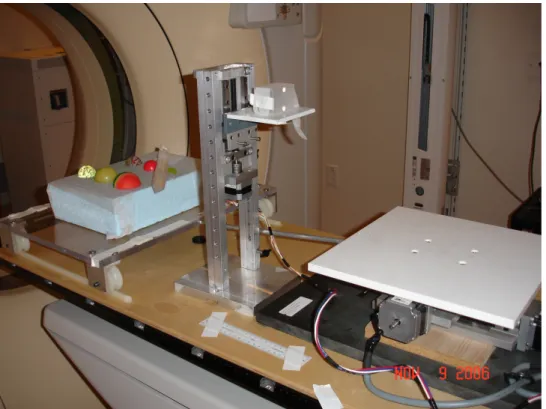
in a 1-Dimensional back and forth motion according to the breathing trace. The motion of the sled moved in a cranial-caudal direction along the CT scanner couch to simulate internal organ motion during patient respiration. A second stepping motor assembly synchronously translated a horizontal ledge in the vertical axis to simulate abdominal surface motion during respiration. For the GE scanner experiments, the Varian RPM system was used to track the motion. Figure 3-1 shows the phantom on the computer-driven sled along with a Varian RPM marker box placed on the ledge.
Figure 3-1: Phantom positioned on the computer-driven sled, which was used in the 4D CT experiments.
In the experiments using the GE scanner, a Varian RPM marker box was placed on the ledge of the motion simulator. As explained in Section 2.2.2, the RPM system tracks the motion of this marker box to monitor breathing. 4D CT images were reconstructed at ten phases of respiration, which are referred to as 0%, 10%, 20%, . . . , 90% phase. The convention is that 50% phase is at full exhale, and 0% phase is at full inhale in the respiratory cycle. However, when using the GE scanner, the RPM software inverts this convention so that 50% is at inhale and 0% is at exhale.
In this thesis, any data dealing with the GE scanner will use the convention that 50% phase is at inhale and 0% phase is at exhale.
3.1.2
Philips CT Scanner
The same phantom and computer-driven sled was used for the Philips scanner exper-iments as was used with the GE scanner experexper-iments. However, a different breathing monitor was used to track phantom motion. In the experiments using the Philips scanner, the bellows device (belt) was wrapped around the bottom of the motion simulator and the ledge. The vertical motion of the ledge caused the belt to expand and contract, which allowed the bellows device to monitor the motion, as explained in Section 2.2.2.
Similar to the GE experiments, 4D CT images were reconstructed at ten phases of respiration, which are referred to as 0%, 10%, 20%, . . . , 90% phase. The convention with the Philips scanner is that 0% phase is at full inhale, and 50% phase is at full exhale in the respiratory cycle. Note that this convention is opposite that of the convention used in this thesis for the GE scanner, as mentioned in Section 3.1.1.
3.1.3
Breathing Traces
The breathing traces used to simulate irregular breathing were previously recorded from patients undergoing 4D CT scans using the GE scanner. As a result, these recorded traces were stored in the RPM data file format. An RPM breathing trace file is a text file that specifies the amplitude of the marker box as a function of the recorded time. Along with some information about the CT scan in the header, the file includes the RPM-assigned phase of the trace as a function of time and the instances along the trace when the x-ray beam was enabled.
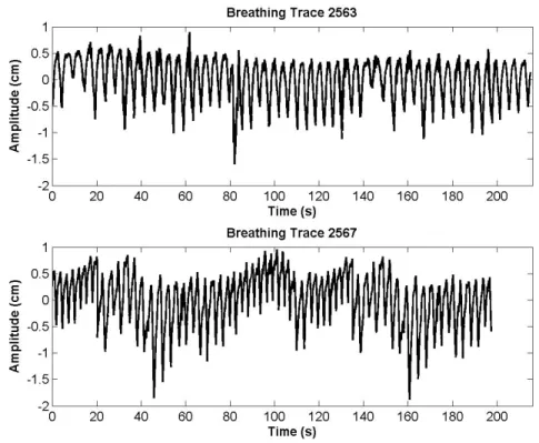
Two traces were used, each from a different patient, to simulate irregular respira-tory motion, and they are identified as breathing trace 2563 and breathing trace 2567. Although traces 2563 and 2567 were recorded using the RPM system and contained phase and beam-on information from the patient scans, only the amplitude
informa-tion was used to drive the phantom for the experiments. The phase and beam-on information were recalculated by the breathing monitor during or after the scan, for the GE or Philips scanner, respectively.
The amplitude of each recorded RPM trace depends on the placement of the RPM box on each patient’s abdomen. For example, the amplitude measured by the RPM system may be smaller if the box is placed lower on the abdomen where motion due to breathing is less pronounced. The internal organ motion obviously does not depend on the placement of the box. However, if the box is placed at a location with greater motion, the measured motion of the box is larger. Therefore, since the breathing traces are used to drive the phantom (internal organ) motion, each breathing trace is multiplied by a chosen scale factor in order to make the phantom motion more realistic. A scale factor of 3 was used for the 2563 trace, and a scale factor of 2 was used for the 2567 trace. These traces are shown in Figure 3-2.
Figure 3-2: Breathing traces 2563 (displayed using a scale factor of 3) and 2567 (displayed using a scale factor of 2). The peaks of the traces correspond to exhale and the valleys correspond to inhale.
In addition, a 2 cm peak-to-peak sine waveform and a 1 cm peak-to-peak sine waveform were used to drive the phantom. Since these sinusoidal traces were created using a computer, they were already in the amplitude versus time format. Breathing traces 2563, 2567, 2 cm sine, and 1 cm sine were used to drive the phantom for both the GE scanner experiments and the Philips scanner experiments.
3.1.4
Breathing Trace Analysis
After performing the GE scanner experiments, the RPM breathing traces, which contain the phase and x-ray beam-on information from the phantom scans, were obtained. This enabled the amplitude-phase relationship to be plotted for each given phase of reconstruction.
Furthermore, a study was performed on 122 different RPM breathing traces recorded from patients in a scanning or treatment hospital environment. These traces were analyzed to determine the average length of time for a cycle of breathing, average baseline drift1, and average variance of breathing cycle amplitudes.
To determine the average breathing period for each trace, the length of time of each cycle of breathing was measured by using the phase information from each recorded RPM trace to determine the breathing cycles for each trace. Then, all the breathing periods were averaged for each trace, and then those averages were averaged to obtain a single number.
To determine the baseline drift and breathing cycle amplitudes, each trace was first normalized to its average amplitude since the amplitude can vary depending on RPM box placement, as discussed in Section 3.1.3. The average amplitude of each trace was computed similarly to the way the average breathing period was computed: the amplitudes of the breathing cycles were averaged, where the breathing cycles were defined by the phase information from the trace. The baseline drift was measured in two ways. The first way was to take the difference between the maximum of the peaks and the minimum of the peaks of the trace. The peaks of the trace were found by examining each breathing cycle and taking the maximum amplitude of each cycle.
The second way to measure baseline drift was to measure the slope of the best fit line of the peaks. Finally, the variance of the measured breathing cycle amplitudes for each trace was computed, and then the variances were averaged.
3.1.5
Error Quantification
In order to quantify the image artifacts obtained from the experiments, the volume of Sphere 1 in each image was calculated for comparison to the true volume of Sphere 1, which was computed using a caliper-measured diameter. Sphere 1 is the largest sphere in the phantom shown in Figure 3-1 and is labeled with the number one in Figure 4-2. The caliper-measured diameter of Sphere 1 is 5.461 cm, which yields a volume of approximately 85.27 cm3.
The image volume of Sphere 1 was calculated from the Philips scanner by first thresholding the 3D image with a pixel value of 200 to create a binary image. The connected objects in the binary image were then labeled by using the bwlabeln() function in MATLAB with a 26-connected neighborhood. The volume of Sphere 1 was simply the number of voxels in the thresholded Sphere 1 image. To convert number of voxels into cubic centimeters, a conversion factor was used that consisted of the caliper-measured volume of Sphere 1 divided by the number of voxels in the static 3D Philips scan of Sphere 1.
In addition to using the previous method to calculate the volume of Sphere 1 in the GE scanner images, the GE Sim4D software tools, which presumably thresholds the objects as well, were also used. However, when the volumes of Sphere 1 generated by the GE scanner were compared to those generated by the Philips scanner, the volumes calculated from the MATLAB method mentioned above were used.
The center of mass (COM) of Sphere 1 was also computed in each of the 4D reconstructed images from both the GE and Philips scanners. The COM of Sphere 1 was computed by averaging the 3D coordinates of each voxel of Sphere 1. For example, for the x-coordinate, the x-coordinates of all the voxels of Sphere 1 were summed together, and then divided by the total number of voxels in Sphere 1. The y-coordinate and z-coordinate of the COM were computed in a similar fashion. Since
each voxel is not a perfect cube, different conversion factors had to be used for each coordinate of the COM to convert into centimeters. The x-coordinate, y-coordinate, and z-coordinate conversion factors consisted of the caliper-measured diameter of Sphere 1 divided by the number of voxels of the diameter of Sphere 1 in the x-direction, y-x-direction, and z-x-direction, respectively. The orientation of the coordinates is as follows: the x-coordinate specifies the row of each axial slice from the DICOM data, the y-coordinate specifies the column of each axial slice, and the z-coordinate specifies the cranial-caudal direction.
3.2
4D CT Simulations
3.2.1
General Electric Scanner Experiment Simulations
Software in the MATLAB programming language was implemented to simulate the 4D CT scanning process used by the GE scanner. Figure 4-15 shows an example of the end result of the simulation. In this simulation, a sphere surface moves along a cranial-caudal trajectory specified by an RPM trace that is multiplied by the scale factor and positioned so that the mean of the trace is at an amplitude of zero. The sphere moves along the trace so that the very center of the sphere corresponds to the given amplitude. The simulation shows an amplitude versus time plot and a phase versus time plot for the duration in which data is acquired. In both of these plots, data acquisition points are marked with crosses, and connected with a dotted line. Couch positions, which are specified by the beam-on and beam-off information from the RPM trace, are indicated in both plots by a square wave that fluctuates between 1 and 0. A value of 1 indicates beam-on and 0 indicates beam-off.
During the simulation, a small circle moves along the amplitude plot to indicate the position of the sphere. An example of this is shown in Figure 4-17 where the small circle is shown at the very end of the amplitude plot since the figure shows the end results of the simulations. At each specified acquisition point when the small circle on the amplitude plot meets a cross, the simulation captures a four-slice section of
the sphere and draws the appropriate section in the coronal view on the left of the two plots. In addition to drawing this four-slice section, the simulation also draws a circle surrounding the acquired section that indicates the true position of the sphere at that data acquisition point. For simplicity, the rotation time of the x-ray source in the simulation is 0 seconds, indicating instantaneous acquisition.
At each consecutive acquisition point, the couch is translated and images are acquired at the next couch position. This process is simulated by slicing the sphere at consecutively lower (caudal) positions. In other words, the simulation gives a stationary couch view of the reconstructed object, while moving the scanning plane in the caudal direction for each consecutive couch position. Finally, a scale is given on the left of the reconstructed sphere that shows the true size of the reconstructed object.
The GE scanner is a four-slice scanner, and the simulation allows the user to spec-ify how thick each four-slice section will be. Other user inputs include the radius of the sphere surface and the scale factor used to convert the RPM trace amplitude into motion of the sphere, as discussed in Section 3.1.3. The user also specifies the exact indices of the RPM trace where data acquisition occurs. Since couch positions are simulated by slicing at consecutively lower (caudal) positions, the user also specifies the acquisition amplitude2 of the first four-slice section. The very top (cranial) slice
of the four-slice section was specified to correspond to the acquisition amplitude. The 4D CT simulation calculates the volume of the reconstructed surface by math-ematically calculating the volume of each four-slice section. Each four-slice section is essentially a cross section of the sphere. The radius of each slice of the four-slice section was first calculated. Figure 3-3 shows a diagram that explains this process. In this figure, the solid circle represents a coronal view of the sphere at an amplitude of zero, and the dashed circle represents the sphere at a data acquisition point. The horizontal line across the dashed circle represents one particular slice of a four-slice acquisition. The objective is to find the radius x of this slice. The acquisition ampli-tude b is known, the ampliampli-tude a of the sphere at this acquisition point is known from
the RPM trace, and the radius r of the sphere is known. A simple application of the Pythagorean theorem yields x. Once the radius of the slice is computed, the volume of that slice can be computed by approximating it as a perfect disk. The volume of the reconstructed image is just the sum of the volumes of the slices.
The 4D CT simulation can produce a movie of the 4D CT process as the sphere moves along the trace and data is acquired. The simulation also can produce images corresponding to frames of the movie.
Figure 3-3: Diagram for volume computation.
3.2.2
Comparison of Simulations to Experiments
The reconstruction of Sphere 1 in the GE 4D CT experiments with breathing trace 2563 was simulated. A four-slice section thickness of 1 cm (4 × 2.5 mm), a scale factor of 3, and a sphere surface with the same radius as that of Sphere 1 (2.3705 cm) were used, and the sphere was driven using the RPM trace 2563 from the GE 4D CT experiment.
In order to simulate the GE experiments closely, the exact indices of the RPM trace where data acquisition of Sphere 1 occurred needed to be found. First, the sorted DICOM images from the GE scanner that correspond to a given phase were
examined. As explained in Section 2.3.1, for each 4D CT scan, the GE scanner outputs a set of unsorted DICOM images given in the order that each axial slice was acquired, and also a set of sorted DICOM images for each phase. These sorted DICOM images are essentially the 4D reconstructed image of the object, and are taken or sorted from the unsorted DICOM image set. These sorted DICOM images do not contain the information of where in the RPM trace they were acquired. However, the unsorted DICOM images of the scan do contain that information. Therefore, for each phase, the sorted DICOM images that sliced through Sphere 1 were selected and matched to the corresponding image in the unsorted set. Once the unsorted DICOM images that were used in the 4D reconstructed image of Sphere 1 were found, the time location in the RPM trace where these slices occurred was computed.
Next, the acquisition amplitude of the first four-slice section that sliced through Sphere 1, as explained in Section 3.2.1, needed to be found. This was done by examining the very top (cranial) of the reconstructed image of Sphere 1 for each phase. Since the GE scanner is a four-slice scanner, it acquires 4 slices at a time for a given rotation; in other words, the first four DICOM images in a sorted set correspond to one acquisition, DICOM images five through eight correspond to another acquisition, and so on. Therefore, if the most cranial slice of Sphere 1 comes from a DICOM image that is a multiple of four, 0.75 cm needs to be added to account for the fact that the four-slice section missed the top of Sphere 1 in the first three slices. Similarly, if the most cranial slice of Sphere 1 comes from a DICOM image n not equal to a multiple of four, (n mod 4 − 1) ∗ 0.25 cm need to be added.
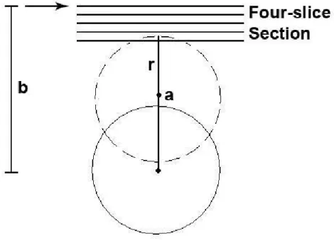
Figure 3-4 shows a diagram that explains this process. The solid circle represents a coronal view of the sphere at an amplitude of zero, and the dashed circle represents the sphere at the first data acquisition point. The horizontal lines across the dashed circle represent the four-slice section, and the arrow points to the acquisition amplitude of the first four-slice section, as explained in Section 3.2.1. To determine the acquisition amplitude b of the first section, the RPM time location of acquisition of the most cranial slice of Sphere 1 was found, which revealed the amplitude a of Sphere 1 at that point in time in the RPM trace. The radius r of Sphere 1 and the extra
space (if any) described earlier was then added to that RPM amplitude to obtain the acquisition amplitude b of the first four-slice section of Sphere 1.
Figure 3-4: Diagram for computation of the acquisition amplitude of the first four-slice section that four-slices through Sphere 1.
3.2.3
Time Shift Simulations
The 4D CT simulation was extended to reconstruct images of Sphere 1 when shifting the start time of scanning. The quality of a 4D CT image depends on the behavior of the breathing trace during the scan, and a patient’s breathing trace can change drastically over a two minute period. Therefore, an investigation of the effects of shifting the start time of scanning was performed, since this time shift will cause the x-ray beam to image Sphere 1 during a different segment of the trace.
This version of the simulation has a number of differences from the previous ver-sion. The user does not specify the exact indices of the RPM trace where data acquisition of Sphere 1 occurs. Instead, he specifies one of ten phases (0%, 10%, 20%, . . ., 90%) and the simulation chooses the data acquisition points using the phase and beam-on information from the RPM trace. Basically, the simulation chooses the point
in each couch position that is closest to the desired phase. The user, however, still needs to specify the acquisition amplitude of the first four-slice section that slices through Sphere 1.
Another difference between this version of the simulation and previous versions is that the user must specify the start time of scanning. The user chooses a point in the RPM trace to start scanning from. If that point is within a couch position, the simulation uses that couch position as the first one for data acquisition. If the starting point is between couch positions, the simulation uses the very next couch position as the first one.
The simulation also allows the user to shift the scanning of couch positions by different amounts of time. The length of each couch position stays the same; each one is just shifted over by the user-specified amount. However, this feature was not explored for the time shift simulations done for this thesis. The couch positions specified by the 2563 trace were used as the different starting points of scanning.
3.2.4
Hysteresis
One major assumption made by the simulation (and 4D CT in general) is that the internal organ motion has a one-to-one correlation with the external motion of the abdomen. In other words, the simulation assumes that, within a scale factor, anterior-posterior movement of the abdomen indicates the exact same internal organ movement in the cranial-caudal direction. This is important because in 4D CT, images are reconstructed based on the amplitude and phase information from external abdominal motion. The true motion of the tumor may be slightly different from the external motion.
Fluoroscopic studies have been performed on patients in order to study the rela-tionship between the external abdominal motion and the internal organ motion during scanning [9]. These studies indicate that hysteresis occurs between the internal and external motion of a patient. In other words, the internal organ motion actually leads the abdominal surface motion by a length of time up to approximately 220 ms. This hysteresis was simulated by having the internal motion lead the external motion by
some length of time specified by the user. Therefore, the data acquisition points ob-tained by the simulation were based on phase information that was delayed in time with respect to the true motion of Sphere 1. For example, if the desired reconstruction phase was 50%, the amplitude of Sphere 1 at an acquisition point would correspond to a point on the RPM trace that was actually a few ms after the true 50% point for that couch position. Simulations using the 2563 breathing trace with delays of 31, 63, 94, 125, 156, 188, 219, and 250 ms were performed.
This version of the simulation that implements the hysteresis delay was based on the previous time shift version described in Section 3.2.3. Therefore, the features and overall algorithm of that simulation were incorporated into this version.
3.2.5
Baseline Drift
Since baseline drift was observed in the breathing traces of patients, the effect of breathing trace baseline drift on the 4D reconstruction of Sphere 1 was studied. Baseline drift introduces variation in amplitude for a given respiratory phase, even if the assigned phase of the breathing trace is accurate. Figure 3-5 shows an example of positive slope creating baseline drift in a breathing trace. In this figure, the exhale points along the baseline drift trace have consecutively increasing amplitudes. If the positive slope were increased, which would result in a more severe baseline drift, the amplitude at the exhale points would increase at an even faster rate. The results of using a breathing trace with varying amounts of positive slope was investigated.
Varying amounts of baseline drift were added to the 2 cm sine breathing trace before using it for the 4D CT reconstruction of Sphere 1. This version of the simula-tion incorporated all the features of the previous versions described in secsimula-tions 3.2.3 and 3.2.4, along with a user-specified input of baseline drift slope. Simulations using the 2 cm sine trace with added drift slopes of 0, 0.0136, 0.0268, and 0.0400 cm/s were performed, and the volumes of these reconstructed images were computed.
Figure 3-5: Example of baseline drift in a breathing trace. The black trace is the original sinusoidal breathing trace. The red dotted trace has a positive slope, resulting in baseline drift. The orientation of the traces is such that the peaks correspond to exhale, and the valleys correspond to inhale.
3.2.6
Arbitrary Object Simulations
The 4D CT simulation was extended to reconstruct objects of arbitrary size and shape. Previous versions of the simulation only had the capability of using a sphere surface to simulate the tumor shape. Since tumors exist in a wide variety of shapes, another version of the simulation was implemented that, in addition to the features of scan start time shift, hysteresis of internal and external motion, and baseline drift, was able to take in an arbitrary object and perform a 4D CT scan using an RPM breathing trace.
The simulation takes in as input a Dimensional matrix that represents the 3-Dimensional object to be scanned. This 3-D matrix is a stack of axial slices of the object, similar to the DICOM data retrieved from a CT scan. The simulation moves the center of the object along the RPM trace. Similar to some of the previous sphere surface simulations, the user chooses the thickness of each four-slice section, the scale factor used to convert the breathing trace amplitude into actual object motion, and the acquisition amplitude of the first four-slice section that slices through the object, as described in Section 3.2.1. In addition, the user chooses a specific phase for reconstruction, and the simulation picks the data acquisition points using the phase and beam-on information from the RPM trace.
However, there are some additional input parameters specific to the arbitrary object simulation. The simulation needs to know the true size of the input object along the cranial-caudal direction. The simulation needs this information to determine how much of the object is acquired at each four-slice section acquisition. Therefore, the user specifies the number of voxels per centimeter along the cranial-caudal direction of the object.
Although the simulation deals with an arbitrary 3-Dimensional object and pro-duces a 3-Dimensional reconstructed image, it gives a coronal view of the image similar to the previous surface simulations. The arbitrary object simulation allows the user to specify the coronal plane of view during the simulation. Figure 4-22 shows an example of the end result of the simulation. Like the previous surface simulations,
it includes the amplitude and phase plots along with the reconstructed coronal slice. To see how the simulation would perform with respect to our experiments using the GE scanner and to our previous simulations of Sphere 1, the static, 3D scan of Sphere 1 was used as the input object to our simulation. RPM breathing trace 2563 was used to drive the arbitrary object simulation of Sphere 1 for a number of different respiratory phases.
3.3
Radiation Treatment Simulations
Using the software framework implemented for the sphere surface 4D CT simulations, a program that simulates the gated radiation treatment of a patient was developed. During gated radiation treatment, sometimes the patient’s breathing is so irregular that the staff moves the gating window to compensate for baseline drift or amplitude variation. The goal was to use the simulation to determine if the tumor was still being adequately irradiated with these gating window changes.
Figure 4-26 shows an example of the end result of this simulation. This simulation takes in an RPM breathing trace recorded from gated radiation treatment and moves a circle corresponding to the tumor along the trace. The RPM breathing trace obtained from gated radiation treatment contains the amplitude and phase information of the abdominal surface trajectory, and also the instances when the x-ray treatment beam was on. Figure 4-25 is an example of the RPM trace obtained from gated radiation treatment. The red dots indicate points where the treatment beam was enabled. Since the treatment was gated based on amplitude, the discontinuities of the red dot baseline indicate the instances when the gating window was shifted. For example, there was a clear gating window change at approximately 70 to 80 seconds in Figure 4-25.
On the left side of Figure 4-26, the smaller circle represents the tumor while the larger circle represents the aperture of radiation treatment. The larger circle remains stationary, and both the circles start out as blue in color. When the beam is turned on as specified by the RPM trace, the smaller circle representing the tumor turns
red. The smaller circle turns blue when the beam is off. The square wave in both the amplitude and phase plots represents when the beam was turned on and off (1 = on, 0 = off). A small circle moves along the amplitude plot to indicate the position of the sphere during the simulation. Additionally, since the duration of treatment is typically around 10 minutes, the amplitude and phase plots scroll along the trace with a window of around 15 seconds, as shown in Figure 4-26. By examining the position of smaller circle when it turns red, the user can easily view whether or not the entire tumor area is being irradiated by the x-rays.
The simulation allows the user to specify the radius of the tumor and aperture circles, the position (amplitude) of the aperture circle, and the scale factor used to convert the breathing trace amplitude into actual tumor motion. The simulation also allows time shifts of starting scan time, similar to how it was described in Section 3.2.3. This simulation produces a movie of the entire radiation treatment process, and optional images corresponding to specific frames of the movie. Simulations of gated radiation treatment were performed with tumor and aperture radii of 3 and 3.5 cm, respectively, an aperture amplitude of zero, and a scale factor of 1.
Chapter 4
Results
This chapter describes the experimental results of 4D CT using the General Elec-tric (GE) scanner at Massachusetts General Hospital and the Philips scanner at the Boston Medical Center. The breathing traces used to simulate patient breathing dur-ing scanndur-ing are analyzed. The simulation results are presented and compared to the experimental results.
4.1
Breathing Trace Analysis
The quality of a 4D CT scan depends greatly on the characteristics of the breathing trace. In order to capture the irregularities inherent in the breathing patterns of humans, two breathing traces recorded from patients were used: trace 2563 and trace 2567. A perfect 2 cm sine wave breathing trace was used as a comparison. Segments of the 2563, 2567, and 2 cm sine breathing traces, along with their RPM-assigned phases, are shown in Figure 4-1. The segments of traces 2563, 2567, and 2 cm sine in the figure represent the segments of time in which Sphere 1 was scanned by the GE CT scanner. The amplitude plots are oriented such that exhale is at the peaks of the wave, and inhale is at the valleys. In addition, the amplitude plots have been scaled by the internal-external motion scale factor1, discussed in Section 3.1.3, and represent the true motion of the phantom during the experiments.
Figure 4-1: Amplitude, phase, and amplitude phase correlation of traces 2563, 2567, and 2 cm peak to peak sine wave. The segments shown in the figure correspond to segments where Sphere 1 was scanned by the GE scanner. The internal-external motion scale factor is incorporated into the amplitude plots, which correspond to the true motion of the phantom.
The amplitude-phase correlation is shown in the third row of Figure 4-1. This amplitude-phase correlation indicates the amplitude of the breathing trace depicted in the first row at specific phases depicted in the second row. The amplitude-phase correlation is a useful metric to determine the quality of a 4D CT scan based on the breathing trace. Notice that the spread of the amplitudes at each phase for the 2 cm sine trace is much smaller than the spread for the 2563 and 2567 traces. This is expected since a perfect sine wave will have a very predictable amplitude at each given phase of the trace. Additionally, the phase assignment was much more accurate for the 2 cm sine trace due to the regularity of the trace. The accuracy of phase assignment also contributed to the small spread of amplitudes at each phase.
Trace 2563 was chosen for the experiment because of its variation in inhale ampli-tude at different breathing cycles, while having a relatively stable baseline at exhale. However, as shown in Figure 4-1, the segment of the trace in which Sphere 1 was scanned by the GE scanner has a significant breathing irregularity at around 83 sec-onds. This irregularity made it very difficult for the phase assignment software to obtain the correct phases at this point, and as a result, the spacing of the cycles shown in the 2563 phase plot is incorrect. There are some outliers for several phases in the 2563 amplitude-phase plot. Outliers for phases 20%, 30%, and 50% are espe-cially prominent. These outliers are a direct result from the breathing irregularity around 83 seconds. Because the assigned phases were incorrect at this irregularity, the amplitude of Sphere 1 at that irregularity was different from the amplitude at the other couch positions for phases 20%, 30%, and 50%. Therefore, even though trace 2563 exhibits a relatively stable baseline at exhale, the resulting 4D reconstructed image at exhale is not guaranteed to be artifact-free because of the errors in phase assignment.
Trace 2567, on the other hand, has significant baseline drift while maintaining a somewhat regular breathing cycle amplitude. No significant breathing irregularities occur during the GE scanning of Sphere 1, and the RPM software did not have difficulty assigning phases, as shown in Figure 4-1. The spread of the amplitudes for each phase is due to the varying baseline of trace 2567.
The amplitude plot for the 2 cm sine wave in Figure 4-1 is quite regular, and the RPM software assigns the phases correctly. Looking at the amplitude-phase plot for the 2 cm wave, the points have slightly more spread at phases between 0% (exhale) and 50% (inhale). This is the most noticeable at phases 80% and 90%. This slight variation in amplitude is due to the velocity of the phantom at these phases. At around 0% and 50%, the phantom is changing direction and the velocity of the phantom is around zero. The phantom is traveling the fastest at phases such as 80% and 90%, making the amplitude at these phases vary slightly.
In addition, a study was performed on 122 different breathing traces recorded from patients in a scanning or treatment hospital environment. The average breath-ing period was found to be approximately 3.961 seconds. Since the breathbreath-ing trace amplitude may vary from day to day due to RPM sensor placement on each patient, the amplitude of each trace was normalized to the average breathing cycle amplitude for that trace. The average baseline drift in terms of the peaks of the trace was 0.5634. The average baseline drift in terms of slope was 4.2642 · 10−4. The average variance of the breathing cycle amplitudes was 0.06303. No scale factor was used for this analysis, and Table 4.1 summarizes these results.
Table 4.1: Characteristics of 122 different breathing traces. No scale factor was used.
Average Breathing Period 4.0 s
Average Baseline Drift (Peaks) 0.56 (no units)
Average Baseline Drift (Slope) 4.3 × 10⁻⁴ s−1
Average Variance of Breathing Cycle Amplitudes 0.063 (no units)
4.2
Experiments
4.2.1
General Electric CT Scanner
This section gives the results of 4D experiments using the moving phantom, GE scanner, and Varian RPM system. Figure 4-2 shows coronal slices of the phantom
taken at 50% (inhale) phase for the 2 cm sine, 2563, and 2567 breathing traces, along with a 3D scan of the static phantom. All images of the phantom were constructed from sorted DICOM data from the scanner, and the coronal slices all intersect the center of Sphere 1.
Figure 4-2: Using the GE scanner, (a) coronal slice of static phantom; coronal slice of phantom at 50% (inhale) phase for (b) 2 cm sine, (c) 2563 trace, (d) 2567 trace.
The 2 cm scan in Figure 4-2b is free of artifacts and resembles the static scan in Figure 4-2a. This is expected given the nature of the 2 cm breathing trace described in Section 4.1. The 2563 scan in Figure 4-2c, however, has a number of significant artifacts. The top section of Sphere 1 in the 2563 scan is smaller than it should be, indicating that the amplitude of the sphere was too low at that data acquisition point. The section of Sphere 1 that is second from the bottom is essentially a duplicate of
the very bottom of the sphere. These artifacts of Sphere 1 can be correlated to the artifacts of the diagonal ruler in the same image.
The 2567 scan in Figure 4-2d appears to have less serious artifacts than those in the 2563 scan. The top of Sphere 1 appears slightly pointed and elongated, and the ruler is not as straight as it is in Figures 4-2a and 4-2b.
The 0% (exhale) phase scans using traces 2563 and 2567 shown in Figure 4-3 appear to have slightly fewer artifacts than the corresponding 50% (inhale) scans. In fact, in Figure 4-3c, only the most bottom section of Sphere 1 appears out of place. The headers of the DICOM image that produced the bottom section of Sphere 1 were searched and it was discovered that this section was acquired during the breathing irregularity of trace 2563, discussed in Section 4.1. Given that the amplitude of trace 2563 at exhale did not vary much, Sphere 1 would have been almost artifact-free without the breathing irregularity that occurred during the scanning of the bottom section.
The 0% (exhale) phase scan using trace 2567 in Figure 4-3 appears slightly better than the inhale scan of 2567. Sphere 1 is slightly elongated and the ruler is not as straight as in the static scan of the phantom, but the overall shapes of the phantom are intact. Examining the 2567 breathing trace in Figure 4-1, the exhale baseline starts a little high, but remains somewhat constant throughout the period of data acquisition for Sphere 1. Figure 4-3 shows that the scan of Sphere 1 reflects the behavior of the breathing trace: the top of Sphere 1 is a slightly elongated due to the exhale baseline starting high, but the rest of the sphere has barely any artifacts due to the exhale baseline remaining relatively constant.
The image volume of Sphere 1 was computed using GE Sim4D tools. Figure 4-4 shows these computed volumes at all ten phases using breathing traces 2563, 2567, 2 cm sine, and 1 cm sine. Variations in the volume range from +12% to -12% of the ground truth volume for trace 2563, which was 85.2737 cm3. Variations for trace 2567
were +6.1% to -6.2%. Sinusoidal breathing traces exhibited less respiratory phase dependence; for a 2 cm amplitude peak to peak, the volume ranged from +7.9% to -3.0%, while for a 1 cm amplitude, the volume ranged from +5.3% to -0.20%.
Figure 4-3: Using the GE scanner, (a) coronal slice of static phantom; coronal slice of phantom at 0% (exhale) phase for (b) 2 cm sine, (c) 2563 trace, (d) 2567 trace.