Control of the Black-Scholes equation

(1)

HAL Id: hal-01448825

https://hal.sorbonne-universite.fr/hal-01448825

Submitted on 29 Jan 2017

HAL is a multi-disciplinary open access

archive for the deposit and dissemination of sci-entific research documents, whether they are pub-lished or not. The documents may come from teaching and research institutions in France or abroad, or from public or private research centers.

L’archive ouverte pluridisciplinaire HAL, est destinée au dépôt et à la diffusion de documents scientifiques de niveau recherche, publiés ou non, émanant des établissements d’enseignement et de recherche français ou étrangers, des laboratoires publics ou privés.

Control of the Black-Scholes equation

Claire David

To cite this version:

Claire David. Control of the Black-Scholes equation. Computers & Mathematics with Applications, Elsevier, 2017. �hal-01448825�

(2)

Control of the Black-Scholes equation

Claire David January 29, 2017

Université Pierre et Marie Curie-Paris 6 Laboratoire Jacques Louis Lions - UMR 7598

Boîte courrier 187, 4 place Jussieu, F-75252 Paris cedex 05, France

Abstract

The purpose of this work is to apply the results developped by J.Y. Chemin and Cl. David [1], [2], to the Black-Scholes equation. This latter equation being directly linked to the heat equation, it enables us to propose a new approach allowing to control properties of the solution by means of a shape parameter.

Key Words: Black-Scholes equation ; control; shape parameters.

1 Introduction

It is well known that the Black-Scholes (BS) model, which gives the dynamic of the option prices in financial markets [3], [4], is given, in its usual arbitrage free version, and the specific case of a "call", for european options, by:

∂tC +σ

2_S2 2

∂2C

∂S2 + r (S ∂SC− C) = 0

where the price of the option, C, is a function of the underlying asset price S and time t; r is the risk-free interest rate, and σ the volatility of the stock.

There are hundreds of papers dealing with the Black-Scholes equation. Yet, no one seems to have ever used the scaling invariance coming from the heat equation. And there appears to be very few studies on the "control aspect" of the equation (one can see, for instance [5]).

In [2], J.Y. Chemin and Cl. David obtained new results for the mass critical nonlinear Schrödinger equation, building a continuous map from the Lebesgue space L2(R2) in the setG of initial data which give birth to global solution in the space L4(R1+2). The principle is simple: one uses the fact that for this nonlinear equation, solutions of scales which are diﬀerent enough almost do not interact. The nonlinearity of the original equation just required to determine a condition about the size of the scale which depends continuously on the data.

The idea is to apply the building technique of the map described above, starting from the point that the Black-Scholes equation can be transformed into a linear heat equation, which has a natural scaling invariance, and that the linearity of the transformed equation enables one to obtain exact solutions, and, thus, yield interesting results. The aim of this paper is to present a new way to change either the Delta, or other greeks, by a given amount ; this technique appears thus as a new way to control the equation, without resorting to control functions. Indeed, one can change the greeks directly using the

(3)

general solution of the Black-Scholes equation, nevertheless, our technique appears as an alternative and simple one to implement.

Section 2 is devoted to applying the Chemin-David technique to the Black-Scholes equation.

The consistency of the approach with respect to initial conditions is examined in Section 2.2.

Section 3 present numerical results.

2 Introduction of a shape parameter

2.1 Classical results for the Black-Scholes equation

If one denotes by E the exercise price of the option, for a study in the time interval [0, T ], T > 0, the limit conditions are:

     C(0, t) = 0 for all t lim S→+∞C(S, t) = S C(S, T ) = max {S − E, 0}

The Black-Scholes equation can classically be transformed into a heat-diﬀusion equation, through the change of variables: τ = σ 2 2 (T − t) , x = ln S E setting: C(S, t) = E eC(x, τ ) and: e C(x, τ ) = eα x+β τC(x, τ )ee where: k = 2 r σ2 , α = 1− k 2 , β = α 2_{+ (k}_{− 1) α − k = −}(k + 1)2 4 which lead to the normalized heat equation:

∂ eCe ∂τ = ∂2Cee ∂x2 ∀ (x, τ) ∈ [ 0,σ 2_T 2 ] × R (1)

with the initial condition: ee C(x, 0) = eCe0(x) = max { e(k+1) x2 − e (k−1) x 2 , 0 } (2) The classical analytical solution is then given by:

ee Cclassical(x, τ ) = 1 2√π τ ∫ _∞ −∞ ee C0(y) exp [ −(x− y)2 4 τ ] dy (3)

(4)

2.2 Our approach - Consistency with respect to initial conditions

Let us recall the natural scaling of the heat equation (1). If we denote by eC a solution, then, for anye

strictly positive real number λ, the map

(t, x)7→ eeCλ(t, x) = λ eC(λe 2t, λx)

is also solution.

Following J.Y. Chemin and Cl. David [1], [2], we define the mapping, denoted byF, from L2_loc(R) × R⋆₊× N⋆, by: F ( ee C0, λ, N0 ) = eCe0+ ϵ N0 ∑ j=1 λ−jCee0 ( λ−j·) , ϵ ∈ {−1, 1} , N0 ∈ N⋆

which takes its origin in the so-called "profile decomposition theory" initiated by P. Gerard and H. Bahouri [6]. It relies on the idea that two solutions of an evolution equations with scales that are diﬀerent enough almost do not interact.

An important question one may ask is wether our approach does not aﬀect the required initial condi-tions (2).

The diﬃculty, here, lays in the fact that the functions at stake are not integrable on R. This is the reason why we will work on L2_loc(R), more precisely, on L2([0, S0]), for S0 > 0.

The main property ofF is given by the proposition that follows.

Proposition 2.1. There exists a strictly positive constant λ0 such that:

λ> λ0 ⇒ F ( ee C0, λ, N0 ) − eeC0 2 L2_([0,S 0]) = o(1) (4)

Proof. One has:

F(Cee0, λ, N0 ) − eeC0 2 L2_([0,S 0]) = N0 ∑ j=1 λ−jCee0 ( λ−j·) 2 L2_([0,S 0]) = N0 ∑ j=1 λ−2j eeC0 ( λ−j·) 2 L2_([0,S 0]) +2 ∑ 16j<k6N0 λ−j−k ( ee C0 ( λ−j·), eCe0 ( λ−k· )) L2_([0,S 0]) 6  ∑N0 j=1 λ−j   _eeC₀ 2 L2_([0,S 0]) +2 ∑ 16j<k6N0 λ−j−k ( ee C0 ( λ−j) · eeC0 ( λ−k )) L2_([0,S 0]) = λ−11− λ −N0 1− λ−1 eeC0 2 L2_([0,S 0]) +2 ∑ 16j<k6N0 λ−j−k ( ee C0 ( λ−j·), eCe0 ( λ−k· )) L2_([0,S 0]) due to:

(5)

λ−2j eeC0 ( λ−j·) 2 L2_([0,S 0]) = λ−2j ∫ S0 0 ee C 2 0 ( λ−j·) dS = λ−2j ∫ λ−jS0 0 ee C 2 0(·) λjdS 6 λ−j ∫ S0 0 ee C 2 0(·) dS = λ−j eeC0 2 L2_([0,S 0])

and, for any set of integers (j, k) ∈ {1, . . . , N0} such that j < k, provided that the scaling factor λ is great enough, the pseudo-orthogonality, or the fact that scales that are diﬀerent enough almost do not interact, yields: λ−j−k ( ee C0 ( λ−j·), eCe0 ( λ−k·)) L2_([0,S 0]) = λ−k ∫ λ−jS0 0 ee C0(·) eeC0 ( λ−(k−j)· ) dS = o(1)

For any strictly positive real number ε, one easily can find the threshold value λ0 such that:

∀ λ > λ0 : λ−1 1− λ−N0 1− λ−1 eeC0 2 L2_([0,S 0]) 6 ε

Remark 2.1. The mapping F shows that the control depends on N0 and λ. As λ increases, one will require smaller values of the integer N0:

N0ln λ6 exp            − 1 N0 ln      1− ε λ 1− λ−1 eeC0 2 L2_([0,S 0])                 

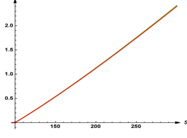
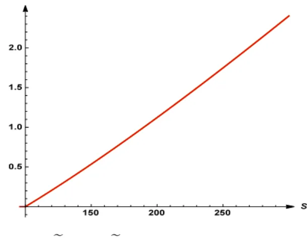
The illustration of the above theoretical results can be seen through the following numerical results. We hereafter display the variations of:

the initial condition function eeC0 given by (2), in red ; the initial condition function eeC0,λ given by:

ee C0,λ(x) = eCe0(x)+ϵ N0 ∑ j=1 ee C0,λ,j(x) = eCe0(x)+ϵ N0 ∑ j=1 1 λj Cee0 (_x λj ) = eCe0(x)+ϵ N0 ∑ j=1 1 λj max { e (k+1) x 2 λj − e (k−1) x 2 λj , 0 } in green ;

in the case where:

r = 0.06 , σ = 0.3 , E = 100

(6)

Figure 1: The graph of eCe0 and eCe0,λ as functions of stock price S, for λ = 2.

2.3 Analytic results

As previously, we consider, for Λ > Λ0, initial data of the form:

ee C0,λ(x) = eCe0(x)+ϵ N0 ∑ j=1 ee C0,λ,j(x) = eCe0(x)+ϵ N0 ∑ j=1 1 λj Cee0 (_x λj ) = eCe0(x)+ϵ N0 ∑ j=1 1 λj max { e (k+1) x 2 λj − e (k−1) x 2 λj , 0 }

The related exact analytic solution eC, which is a function of x, τ , and of the scaling parameter λ, ise

(7)

ee C(x, τ, λ) = eCclassicale (x, τ ) + ϵ 1 2√π τ ∫ +∞ −∞ N0 ∑ j=1 ee C0,λ,j(y) e−(x−y)24 τ dy

(8)

1 2√π τ ∫ +∞ −∞ ee C0,λ,j(y) e− (x−y)2 4 τ dy = √1 π λj ∫ +∞ −∞ max { e (k+1) x 2 λj − e (k−1) x 2 λj , 0 } e−z2dz = √1 π λj ∫ +∞ − x 2√τ e (k+1) (x+2 z√τ ) 2 λj e−z 2 dz −√1 π λj ∫ +∞ − x 2√τ e (k−1) (x+2 z√τ ) 2 λj e−z 2 dz = √1 π λj ∫ +∞ − x 2√τ e (k+1) x 2 λj e− ( z+(k+1)√τ 4 λj )2 dz −√1 π λj ∫ +∞ − x 2√τ e(k−1) x+(k−1)2τe− ( z+(k−1) √ τ 2 λj )2 dz = e (k+1) x 2 λj + (k+1)2 τ 4 λ2j √ π λj ∫ +∞ − x 2√τ e− ( z+(k+1) √ τ 2 λj )2 dz −e (k−1) x 2 λj + (k−1)2 τ 4 λ2j √ π λj ∫ +∞ − x 2√τ e− ( z+(k−1) √ τ 2 λj )2 dz = e (k+1) x 2 λj + (k+1)2 τ 4 λ2j √ π λj ∫ +∞ − x 2√τ+ (k+1)√τ 2 λj e−zdz −e (k−1) x 2 λj + (k−1)2 τ 4 λ2j √ π λj ∫ +∞ − x 2√τ+ (k−1)√τ 2 λj e−z2dz = e (k+1) x 2 λj + (k+1)2 τ 4 λ2j √ π λj √ π 2 Erfc ( − x 2√τ + (k + 1)√τ 2 λj ) −e (k−1) x 2 λj + (k−1)2 τ 4 λ2j √ π λj √ π 2 Erfc ( − x 2√τ + (k− 1)√τ 2 λj ) = 1 λj e (k+1) x 2 λj + (k+1)2 τ 4 λ2j N (√ 2 x 2√τ − √ 2(k + 1) √ τ 2 λj ) −1 λj e (k−1) x 2 λj + (k−1)2 τ 4 λ2j N ( − √ 2 x 2√τ − √ 2(k− 1) √ τ 2 λj )

where the complementary error function Erfc is defined, for any real number x, by:

Erfc(x) = √2

π

∫ +∞

x

e−t2dt

while the normal (gaussian) cumulative distribution function is given, for any real number d, by:

N (d) = √1 2π ∫ d −∞e −t2 2 dt = √1 2π √ 2 ∫ +∞ −_√d 2 e−t2dt = 1 2Erfc ( −√d 2 ) Thus:

(9)

ee C(x, τ, λ) = Cclassicalee (x, τ ) + ϵ N0 ∑ j=1 e (k+1) x 2 λj + (k+1)2 τ 4 λ2j 2 λj Erfc ( − x 2√τ + (k + 1)√τ 2 λj ) −ϵ N1 ∑ j=1 e (k−1) x 2 λj + (k−1)2 τ 4 λ2j 2 λj Erfc ( − x 2√τ + (k− 1)√τ 2 λj )

It is interesting to note that:

ee C(x, τ, λ) = Ceeclassical(x, τ ) + ϵ N0 ∑ j=1 1 λj Ceeclassical (_x λj, τ λ2j )

and to notice, thus, that it includes, as expected, the natural scaling of the heat equation (1).

One easily goes back to the call function C through

C(S, t) = E eC(x, τ ) = E e−α x−β τC(x, τ, λ)ee with x = lnS E

3 Results

In finance, the sensitivity of a portfolio to changes in parameters values can be measured through what commonly call "the Greeks", i.e.:

i. the Delta ∆ = ∂C

∂S ∈ [0, 1], which enables one to quantify the risk, and is thus the most important

Greek.

ii. The Gamma Γ = ∂

2_C

∂S2 > 0.

iii. The Vega (the name of which comes from the form of the greek letter ν) ν = ∂C ∂σ. iv. The Theta Θ = ∂C

∂t . v. The rho ρ = ∂C

∂r.

The good strategy, for traders, is to have delta-neutral positions at least once a day, and, whenever the opportunity arises, to improve the Gamma and the Vega [3].

3.1 Control of the Delta and Gamma

To test our approach, we have choosen to compare, first:

the classical Delta ∆classical and Gamma Γclassical ;

the ones of our approach. Due to the decomposition

ee C(x, τ, λ) = Ceeclassical(x, τ ) + ϵ N0 ∑ j=1 1 λj Ceeclassical (_x λj, τ λ2j )

(10)

the change of variables x = lnS E leads to: ∂C ∂S = ∆eeclassical(x, τ ) + ϵ E S N0 ∑ j=1 1 λj ∂ ∂x [ ee Cclassical (_x λj, τ λ2j )] = ∆eeclassical(x, τ ) + ϵ E S N0 ∑ j=1 1 λj ∂ ∂x [ ee Cclassical (_x λj, τ λ2j )] = ∆eeclassical(x, τ ) + ϵ N0 ∑ j=1 1 λ2 j∆eeclassical (_x λj, τ λ2j ) (5)

where we have set:

ee

∆classical(x, τ ) = ∆classical(S, t) = ∂C ∂S

It appears thus that:

for ϵ = 1, one can increase the Delta; for ϵ = −1, one can decrease the Delta.

In practice, it seems interesting to determine a suitable value λ0 of the shape parameter λ such that:

∆ = (1 + ϵ η0) ∆classical , η0 ∈ ]0, 1[ It can be achieved through a series expansion of the quantity 1

λ2 j ∆eeclassical (_x λj, τ λ2j ) . One has: ee ∆classical(x, τ ) = E S ∂ ∂x [ ee C(x, τ ) ] = E S ∂ ∂x  e (k+1) x 2 + (k+1)2 τ 4 √ π √ π 2 Erfc ( − x 2√τ + (k + 1)√τ 2 )  −E S ∂ ∂x  e (k−1) x 2 + (k−1)2 τ 4 √ π √ π 2 Erfc ( − x 2√τ + (k− 1)√τ 2 )  = E S (k + 1) 2 e(k+1) x2 + (k+1)2 τ 4 √ π √ π 2 Erfc ( − x 2√τ + (k + 1)√τ 2 ) + 1 2√τ E S e(k+1) x2 + (k+1)2 τ 4 √ π e ( − x 2√τ+ (k−1)√τ 2 )2 −E S (k− 1) 2 e(k−1) x2 + (k−1)2 τ 4 √ π √ π 2 Erfc ( − x 2√τ + (k− 1)√τ 2 ) − 1 2√τ E S e(k−1) x2 + (k−1)2 τ 4 √ π e ( − x 2√τ+ (k−1)√τ 2 )2 and, therefore:

(11)

ee ∆ (_x λj, τ λ2j ) = E S (k + 1) 2 e (k+1) x 2λj + (k+1)2 τ 4 λj √ π √ π 2 Erfc ( − x 2 λj√_τ + (k + 1)√τ 2 λj ) + λ j 2√τ E S e (k+1) x 2λj + (k+1)2 τ 4 λj √ π e ( − x 2 λj√τ+ (k−1)√τ 2 λj )2 −E S (k− 1) 2 e (k−1) x 2 λj + (k−1)2 τ 4 λj √ π √ π 2 Erfc ( − x 2 λj√_τ + (k− 1)√τ 2 λj ) − λj 2√τ E S e (k−1) x 2λj + (k−1)2 τ 4 λj √ π e ( − x 2 λj√τ+ (k−1)√τ 2 λj )2 (6)

One requires then the series expansion of the Erfc function in 0, which is given, for z ∈ R, by: Erfc(z) = √2 π +∞ ∑ n=0 (−1)n_z2n+1 (2n + 1) n !

For any integer j in{1, . . . , N0}, a series expansion of the term 2 S e∆e (_x λj, τ λ2j ) ϵ E√π is: 1 λ2 j (k + 1) 2√π (₊_∞ ∑ n=0 (k + 1)nxn 2n_λj n_{n !} ) ( 2 √ π +∞ ∑ n=0 (−1)n (2n + 1) n ! ( − x 2 λj√_τ + (k + 1)√τ 2 λj )2n+1) +λ j √ τ (₊_∞ ∑ n=0 (k + 1)n_xn 2n_λj n_{n !} ) ( 1 + ( − x 2 λj√_τ + (k + 1)√τ 2 λj )2 +O ( 1 λ4j )) −(k− 1) 2√π (₊_∞ ∑ n=0 (k− 1)nxn 2n_λj n_{n !} ) ( 2 √ π +∞ ∑ n=0 (−1)n (2n + 1) n ! ( − x 2 λj√_τ + (k− 1)√τ 2 λj )2n+1) −√λj τ (₊_∞ ∑ n=0 (k− 1)nxn 2n_λj n_{n !} ) (₊_∞ ∑ n=0 1 n ! ( − x 2 λj√_τ + (k− 1)√τ 2 λj )n)

One obtains thus, for a given set (x, τ ), or, in an equivalent way, (S, t), and a given value η0, an equation in λ that can be solved numerically.

In the same way as above, the change of variables x = ln S

E leads to: ∂2C ∂S2 = ∂2C ∂S2 + ϵ E2 S2 N0 ∑ j=1 1 λj ∂ ∂S [ ∂ ∂SCeeclassical (_x λj, τ λ2j )] = eeΓclassical(x, τ ) + ϵ N0 ∑ j=1 1 λ3 j Γclassical (_x λj, τ λ2j ) It appears thus that:

for ϵ = 1, one can increase the Gamma ; for ϵ = −1, one can decrease the Gamma. The interesting point is that, due do the relation (5):

(12)

∂ ∂S[∆− ∆classical] = ϵ N0 ∑ j=1 1 λ3 jΓeeclassical (_x λj, τ λ2j ) this expression being of the same sign as ϵ. Hence:

for ϵ = 1, the positive quantity ∆ − ∆classical is an increasing function of the asset stock price S;

for ϵ = −1, the negative quantity ∆ − ∆classical is a decreasing function of the asset stock price S.

It appears thus that if one finds a value λ0 of the scale parameter such that

∆ = (1 + η0) ∆classical , η0 ∈ ]0, 1[, one will increase the Delta on the study interval ; ∆ = (1 − η0) ∆classical , η0 ∈ ]0, 1[, one will decrease the Delta on the study interval.

3.2 Numerical results

We present, in the following, a few numerical results. Tests have been made for:

r = 0.06 , σ = 0.3 , E = 100 , T = 60 days

The following figures display the graph of the diﬀerence ∆− ∆classical as a function of stock price S and time t, for the values of the shape parameter λ such that, at the time T

2, for S = 100: ∆ − ∆classical = 0.15, which leads to the choice λ = 2.37163 ;

∆ − ∆classical = 0.25, which leads to the choice λ = 1.91079 ;

(13)

Figure 6: The graph of the diﬀerence ∆− ∆classical as a function of stock price S and time t, for

λ = 2.37163.

λ = 1.91079.

References

[1] Chemin, J.Y., David, Cl., Sur la construction de grandes solutions pour des équations de Schrödinger de type " masse critique ", Séminaire Laurent Schwartz - EDP et applica-tions, 2013, under press.

[2] Chemin, J.Y., David, Cl., From an initial data to a global solution of the nonlinear Schrödinger equation: a building process, International Mathematics Research Notices, 2015, rnv199, doi:10.1093/imrn/rnv199.

(14)

λ = 1.67543.

[3] Black, F., & Scholes, M., The Pricing of Options and Corporate Liabilities,J. Pol. Econ., 81 ,

1973, 637-659.

[4] Merton, R.C. , Theory of Rational Option Pricing,Bell J. Econ. and Management Sci., 4 ,

1973, 141-183.

[5] Fey, R., & and Polte, U., Nonlinear Black-Scholes equations in finance: associated control problems and properties of solutions,SIAM J. Control optim., 49 (1), 2011, 185-204.

[6] H. Bahouri and P. Gérard, High frequency approximation of solutions to critical nonlinear wave equations, American Journal of Math., 121 , 1999, 131-175.