A continuous real-time interactive basin simulator (RIBS)

A Continuous Real-Time Interactive Basin Simulator

(RIBS)

by

Valeri Yuryevich Ivanov

Submitted to the Department of Civil and Environmental Engineering

in partial fulfillment of the requirements for the degree of

Master of Science in Civil and Environmental Engineering

at the

MASSACHUSETTS INSTITUTE OF TECHNOLOGY

June 2002

@ Massachusetts Institute of Technology, 2002. All Rights Reserved.

A u th or ...

Department of Civil and Environmental Engineering

June, 2002

C ertified by ...

...

Rafael L. Bras

Bacardi and Stockholm Water Foundations Professor,

Department of Civil and Environmental Engineering

Thesis Supervisor

Accepted by ... .. . ... '"...

Oral Buyukozturk

Department of Civil and Environmental Engineering

OF TE~lILLL

CNBLOGY

JUN

3 2002

LIBRARIES

ARCHIVES

A Continuous Real-Time Interactive Basin Simulator

(RIBS)

by

Valeri Yuryevich Ivanov

Submitted to the Department of Civil and Environmental Engineering on May 9, 2002, in partial fulfillment of the

requirements for the degree of

Master of Science in Civil and Environmental Engineering

Abstract

This thesis presents enhancements to a rainfall-runoff, event-based model, the Real-Time Interactive Basin Simulator (RIBS). Major modifications are made in the description of infiltration and subsurface saturated lateral exchange processes. The infiltration model is revised to include a modified Green-Ampt scheme which allows one to account for the cap-illary effects during infiltration in a soil that has exponential decay of the saturated conduc-tivity with depth. A soil moisture redistribution scheme is incorporated in the model to provide a way of simulating the dynamics of the soil moisture profile during interstorm periods. Also added is the capability of modeling the processes of lateral moisture transfer in the ground water system. An unsaturated zone - ground water coupling mechanism is implemented to account for interdependences between the two systems. All these newly added features ensure the capability of the model in applications over longer periods of time under a broader range of meteorological conditions.

Another aspect of the presented work is estimation of the basin state at the beginning of a storm. A new soil moisture initialization scheme is implemented which is different from the kinematic parameterization of the soil water profile used in the previous version of the model. The initial soil moisture profile is linked to the position of the saturated zone. An independent algorithm is developed that obtains the spatial distribution of the depth to the water table in a basin based on a steady state assumption of the topography controlled ground water.

This thesis presents simulations that test each of the model components. Various infiltration events are used to illustrate the sub-grid pixel behavior corresponding to ponded infiltration and infiltration under conditions of rainfall with constant and variable intensity. The ground water simulations are compared with the 2-D analytical solutions of a linearized form of the Boussinesq's equation. The overall model performance is demonstrated in applications for an artificial 1-D hillslope model and a natural watershed. These tests show the model's capability to simulate the principal phases of hydrologic response of a system that couples the unsaturated zone and ground water. Overall, the presented simulation results are physically sound and encouraging.

Thesis Supervisor: Rafael L. Bras

Acknowledgments

I gratefully acknowledge the National Aeronatics and Space Administration (NASA) and

the Department of Civil and Environmental Engineering for the financial support of this work.

I am particularly grateful for the continued guidance and support of my advisor

Rafael Bras who has been coaching me all that time spent at MIT. I thank Dara Entekhabi who provided valuable suggestions and assistance throughout the work. I am grateful to people from Parsons Lab, its current "residents" and alumni, whose work and advice helped in completing this thesis. Special acknowledgements deserve Scott Rybarczyk, Enrique Vivoni, Nicole Gasparini, Greg Tucker, Jingfeng Wang, Vanessa Teles, Jean Fitzmaurice, Frederic Chagnon, and Daniel Collins. I would like to thank Luis Garrote and Mariza Cabral who I have never had a chance to meet. I am very much grateful to the Department of Hydrology at Moscow State University where I spent wonderful years "learning rivers", my former advisor Victor Zhuk in particular. Lastly, special words of gratitude deserve my family and my wife Tatyana.

Contents

I

1.1 Introduction, motivation, and scope of the work ... 13

1.2 R elevant literature ... 16

II Core Model and Its Modifications 23 2.1 Infiltration and runoff generation scheme ... 23

2.1.1 Basin representation ... 23

2.1.2 Runoff generation ... 25

-Basic Assumptions ... 25

-Infiltration Model Description ... 28

Saturated infiltration ... 30

Unsaturated infiltration ... 32

Evolution of fronts ... 37

-Subsurface flow exchange ... 39

-Runoff generation schematic ... 41

2.1.3 Surface flow routing scheme ... 44

2.2 Transformation to a continuous operation ... 47

2.2.1 Soil water redistribution and subtraction... 48

2.2.2 Coupling procedure between fronts of the unsaturated zone and w ater tab le ... 53

2.3 Ground water model description ... 54

2.3.1 Formulation of the ground water model ... 54

2.3.2 Ground water flow partitioning ... 57

2.4 Modifications of the ground water module allowing continuous operation ... 6 1 III Initialization Schemes 71 3.1 Fixing the water table depth: overview of strategies and a modified approach of steady-state ground water distribution ... 71

3.2 An overview of soil moisture initialization schemes. Hydrostatic equilibrium moisture profile ... 77

IV Model Performance: Synthetic Off-line Tests 87 4.1 Test case: ponded infiltration into a semi-infinite soil column ... 87

4.2 Test case: rainfall of constant and variable intensity ... 93

4.3 Ground water model off-line testing ... 101

4.3.1 Damping of a ground water mound in the infinite plane ... 101

4.3.2 Instantaneous filling of a canal: semi-infinite case ... 108 V Model Performance: On-line Model Applications 113 5.1 Test case: the hillslope model ... 113

5.1.1 T he w et case ... 1 14 5.1.2 T he dry case... 1 19

5.2 Test case: Peacheater Creek Basin ... 131

VI Conclusions 141

6.1 Summary of development and implementation results ... 141 6.2 Summary of simulation results ... 143 Appendix 1

The Green-Ampt model for non-uniform soils. Formulation of the

wet-ting front capillary drive ... 145

Appendix 2

Formulation of the wetting front capillary drive for the unsaturated

infil-tration case ... 15 7

Appendix 3

Derivation of an equation for evolution of the top front of the perched

sat-urated zon e ... 159 Appendix 4

Derivation of an equation for the water table depth given the soil moisture

d eficit ... 16 3

Appendix 5

Subtraction and addition of moisture above/below the wetting front in the

perched saturated zone ... 165

List of Figures

2.1 RIBS representation of a subgrid element ... 24

2.2 Schematic representation of the computational element vertical structure w ithin the RIB S ... 32

2.3 Schematic representation of the computational element in the unsaturated zone ... 36

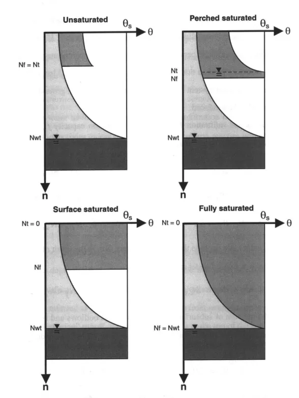
2.4 Four basic pixel states: Unsaturated, Perched Saturated, Surface Saturated, and Fully Saturated ... 44

2.5 Schematic representation of a flow path for a hillslope node ... 46

2.6 Illustration of the module estimating water table drop from the soil surface ... .... 4 9 2.7 Illustration of the module computing water table drop in a cell having initial ground water level at some depth below the soil surface ... 50

2.8 Illustration of the basic drying cycle ... 50

2.9 Illustration of direct water table re-adjustment ... 52

2.10 Computation of flow direction on planar triangular facets ... 60

2.11 Flow partitioning across edges of rectangular box ... 61

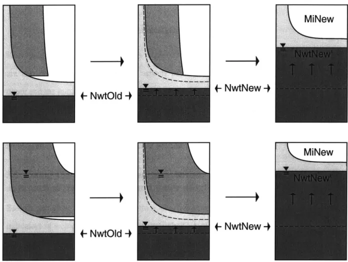
2.12 Illustration of the module accounting for the transition into the saturated state caused by the ground water influx ... 62

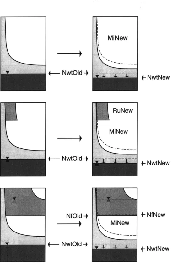
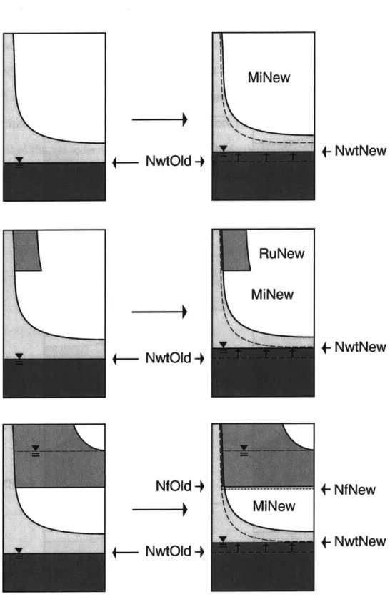
2.13 Illustration of the module accounting for the water table drop in the unsaturated zone -ground water coupling scheme ... 67

2.14 Illustration of the module accounting for the water table rise in the unsaturated zone -ground water coupling scheme. Part I. ... 68

2.15 Illustration of the module accounting for the water table rise in the unsaturated zone -ground water coupling scheme. Part II. ... 69

3.1 Groundwater topography before the smoothing procedure ... 76

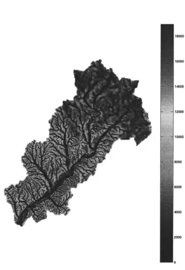
3.2 Estimated depth to the water table. Peacheater Creek, OK ... 77

3.3 Surface soil moisture variation of hydrostatic profile depending on depth to the water table (soil properties represented by the Brooks-Corey param eterization) ... 82

3.4 Surface soil moisture corresponding to the hydrostatic assumption of pressure distribution in (Touchet silt loam, Brooks-Corey parameter-ization) ... ... 83

3.5 Soil moisture distribution corresponding to the hydrostatic assumption

in Brooks-Corey soils ... 84

4.1 Ponded infiltration: base case ... 89

4.2 Ponded infiltration:

f

4.3 Ponded infiltration: 19b parameter varied ... 91

4.4 Ponded infiltration: shallow water table ... 92

4.5 Simulation of infiltration: constant rainfall of 4 mm/hour intensity ... 96

4.6 Simulation of infiltration: constant rainfall of 10 mm/hour intensity ... 97

4.7 Simulation of infiltration: constant rainfall of 20 mm/hour intensity ... 98

4.8 Simulation of infiltration: rainfall of variable intensity, deep water table ca se ...----... 9 9 4.9 Simulation of infiltration: rainfall of variable intensity, shallow water tab le case ... 10 0 4.10 Ground water mound ... 102

4.11 Water table head for simulation run time 50 hours and 240 hours: MS approach ... 104

4.12 Water table head for simulation run time 50 hours and 240 hours: Doo app ro ach ... 10 5 4.13 The error surfaces: Hour 50 ... 106

4.14 The error surfaces: Hour 150 ... 107

4.15 Water table head for simulation run time 240 hours: both approaches ... 110

4.16 The error surfaces: Hour 50 ... 111

4.17 The error surfaces: Hour 240 ... 112

5.1 Representation of an artificial hillslope ... 121

5.2 Cross-sectional view of the hillslope: end of 11-hour 1 mm/hour rain-fall period (w et case) ... 122

5.3 Cross-sectional view of the hillslope: end of 18-hour no-rainfall period (w et case) ... . ... 123

5.4 Cross-sectional view of the hillslope: end of 16-hour 1 mm/hour evap-oration period (wet case) ... 124

5.5 Cross-sectional view of the hillslope: end of 14th hour of 16-hour 10 mm/hour rainfall event (wet case) ... 125

5.6 Cross-sectional view of the hillslope: end of 10-hour 3 mm/hour

evapo-ration period (w et case) ... 126

5.7 Hyetograph and hydrograph for the hillslope simulation (wet case) ... 127

5.8 Cross-sectional view of the hillslope: end of 14th hour of 16-hour 10 mm/hour rainfall event (dry case) ... 128

5.9 Cross-sectional view of the hillslope: end of 10-hour 3 mm/hour evapo-ration period (dry case) ... 129

5.10 Hyetograph and hydrograph for the hillslope simulation (dry case) ... 130

5.11 Surface topography of the Peacheater Creek watershed ... 131

5.12 Summary plot for Peacheater Creek calibration ... 135

5.13 Peacheater Creek: water table at the surface (simulation results) ... 136

5.14 Peacheater Creek: runoff generation (simulation results) ... 137

5.15 Peacheater Creek: subgrid pixel behavior, Case 1 ... 138

5.16 Peacheater Creek: subgrid pixel behavior, Case 2 ... 139

5.17 Peacheater Creek: subgrid pixel behavior, Case 3 ... 140

AL.1 Example of pressure distribution in the saturated thickness ... 147

Al.2 A sketch of the general and the Green-Ampt soil moisture profiles ... 149

Al.3 Sensitivity of the capillary drive term to various parameters ... 155

Al.4 Fit of the model to the data of Childs and Bybordi [1969] ... 156

A3.1 An illustration of the domain of interest Q ... 159

CHAPTER I

Introduction

1.1 Introduction, motivation, and scope of the work

Within the last decade new distributed data sources have created a real wealth of informa-tion for hydrologists. Among the major components significant to flood forecasting capa-bilities was the establishment of the Next Generation Weather Radar (NEXRAD) which provides radar-generated rainfall maps and facilitates gradual improvement of quantitative precipitation forecasts (Olson et al., (1995)). Information about geometry, topography and soil properties of river basins has become readily available from the USGS Digital Eleva-tion Models (DEM), various soils and land use databases such as the Soil ConservaEleva-tion Ser-vice (SCS) State Soil Geographic Databases (STATSGO, SSURGO), the USGS Land Use and Land Cover (LULC) database, and many other local data banks supported by different scientific communities. The level of detail and precision of this type of information have undergone considerable re-evaluation and changes (e.g. Farr et al., 2000) in recent years providing a real wealth of data to flood forecasters. Introduction of these new technologies calls for the improvement of forecasting skills of rainfall-runoff models by using all avail-able information describing the spatial heterogeneity of the land surface and hydrometeoro-logical forcing. Accordingly, recent research efforts in the flood forecasting area have been focused on distributed hydrologic modeling schemes.

The possibility to include detailed basin information on topography, soil types, veg-etative cover, and geology and make effective use of radar-generated rainfall estimates is a promising and attractive opportunity for flood forecasting. Topography has been proven to affect runoff generation significantly, in particular peak streamflow. The soil type and vege-tation cover/ land use type may characterize highly permeable top soil horizons or crusty surface layers that have low water conductivity. The combined effect of accounting for soil type and land use along with moisture availability allows one to describe different runoff

production mechanisms and the state of the basin during various phases of the hydrologic regime. Watershed geologic structure determines the ground water aquifer(s) characteris-tics and influences the catchment baseflow features. All these factors have important impli-cation in physically-based modeling of the processes of runoff generation, infiltration, subsurface lateral moisture exchange, and evapotranspiration in a system that is considered to be spatially non-uniform.

One of the approaches used in the distributed hydrologic modeling is raster-based modeling where spatial heterogeneities in the basin are described using conventional rectan-gular grids. The hydrologic properties are assigned to the center of each node which allows for convenient representation of topography, drainage network, soil types, and land use. A member of this class of rainfall-runoff models is the distributed hydrologic simulation pack-age RIBS, the Real-Time Interactive Basin Simulator, developed by Garrote, [1993], Gar-rote and Bras [1995 a,b]. Its original version is an event-based model which accounts for the effects of slope and soil vertical and horizontal heterogeneity through a simplified for-mulation of the infiltration process and lateral exchange in the unsaturated zone. It offers an integrated software package allowing for distributed raster-based hydrologic simulation within a graphic environment.

However, event-based modeling has a limited scope in practical applications. A model that is intended for use in flood forecasting must be capable of simulating principal hydrologic processes during extended periods of time. It must account for various transi-tion stages of the basin and consider the processes of soil moisture redistributransi-tion and recharge to the ground water system, saturated lateral exchange in the phreatic aquifer, and evapotranspiration. The following chapters in this work deal with developments that signif-icantly enhance the simulation capabilities of the RIBS model, converting it to a continuous simulation model.

Chapter 2 of this thesis extends the infiltration model of Cabral et al. [1992] to include a modified Green-Ampt scheme that is applied for a soil in which the saturated

con-ductivity exponentially decays with depth. It also supplements the infiltration model with a soil moisture redistribution scheme that provides a physically reasonable way to mimic the dynamics of the soil moisture profile during a rainfall hiatus and interstorm periods. A new parameterization is added that allows for extraction of moisture from a soil water profile, therefore simulating evaporation conditions. These procedures significantly expand the range of meteorological conditions under which the model can be used. The model of Gar-rote [1993], GarGar-rote and Bras [1995 a,b] has also been extended to incorporate a ground water module that simulates the lateral fluxes in the saturated zone. Chapter 2 also gives a description of development of an unsaturated zone - ground water coupling scheme that simulates interaction of moving fronts and changing ground water level. The scheme ensures the capability of the model in applications over long periods of time.

Chapter 3 deals with the basin initialization models. It provides a general overview of various approaches for specifying the soil moisture state and ground water level distribu-tion at the beginning of a simuladistribu-tion. An approach using a steady state assumpdistribu-tion of topography controlled ground water (Sivapalan et al., 1987) is described in more detail. It is used as a RIBS input procedure to initialize depth to the water table in a basin. The approximation uses soil hydraulic properties, topography information, and a mean depth to the water table in a catchment. It is further assumed that location of the ground water level

significantly controls wetness conditions in the basin. Knowledge of the water table depth is related to the distribution of moisture in the unsaturated zone. The model uses the hydro-static equilibrium parameterization for the vertical distribution of pressure head which cor-responds to zero initial flux in the unsaturated zone. The Brooks-Corey parameterization of soil hydraulic properties defines the corresponding initialization soil moisture profile in the form of convenient for treatment closed-form expression.

Chapter 4 presents off-line tests of the infiltration model applied to a horizontal lat-erally infinite soil column in which the saturated conductivity is assumed to decay with depth. First, a ponded infiltration case is discussed which demonstrates the general validity

of the modified Green-Ampt scheme. Soil response to constant rainfall intensities of vari-ous magnitude is also simulated. The unsaturated, perched, and surface saturated phases of infiltration are discussed and the conceptual validity of the model is shown. The simulation results for a sequence of storm and interstorm periods are also presented which demonstrate the capability to run the model continuously. Two ground water flow partitioning schemes considered by the model are compared in this chapter. Analytical solutions for 2-D cases are used as a benchmark in these simulations.

Chapter 5 applies RIBS to a synthetic one-dimensional hillslope to evaluate how realistically the model simulates infiltration and subsurface lateral exchange in the unsatur-ated and saturunsatur-ated zones. The simulation includes rainfall and evaporation periods. The dynamics of the principal variables is discussed for two cases: initially wet and dry. The results indicate a general agreement between the model behavior and the expected response in the hillslope system.

A single calibration example is presented for Peacheater Creek basin in Oklahoma.

The model is applied for an event that includes a storm hiatus and interstorm period. Using NEXRAD rainfall data the calibration of the simulated streamflow is performed. The fit of the model output to the observed storm flow is found to be reasonably good, and the cali-brated parameter values are within a physically reliable range. Several cases of subgrid model behavior are illustrated for pixels located in different regions of the catchment. They demonstrate the general consistency of the simulations with hypothesized dynamics in vari-ous hillslope sections.

This thesis presents a work in progress, and its current conclusions and suggestions for further investigation are given in Chapter 6.

1.2 Relevant literature

The model development described in the current work covers a rather broad range of topics. Relevant references are given in this section that are good as general introduction to the

approaches used in the description of hydrologic processes and becoming familiar with the area of distributed rainfall-runoff modeling. Specific literature references are also given in the chapters and appendices of this thesis.

Extensive literature exists on infiltration. Philip [1957] presents a detailed analysis of the theory of flow through unsaturated porous media applied to the problem of infiltra-tion. Analytical solutions for Richard's equations exist only for unrealistic assumptions based on the adoption of a uniform soil moisture with depth and constant positive moisture flux into the soil (e.g. Philip, 1957; Parlange, 1971; Broadbridge and White, 1988; White and Broadbridge, 1988; Warrick et al., 1990). An exact analytical solution for a continuous infiltration process within a given storm of variable intensity is not available. Approximate, physically based approaches for continuous infiltration events have been developed (e.g. Green and Ampt, 1911; Mein and Larson, 1973; Smith and Parlange, 1978; Parlange et al.,

1982; Smith and Hebbert, 1993; Smith et al., 1993; Corradini, et al., 1994). These approx-imate approaches extend to variable rainfall rates and some of them account for soil water redistribution during dry periods (Corradini, et al., 1994; Ogden and Saghafian, 1997). Skaags and Khaleel [1982] and Singh [1989] provide reviews of conceptual and empirical infiltration models used to estimate rainfall excess under one-dimensional and lumped approaches.

The extension of the one-dimensional infiltration problem to the two-dimensional analysis of flow in a hillslope has also been extensively studied. The vertical infiltration in this case is combined with the lateral subsurface flow in the unsaturated and saturated zones. Freeze [1972] made an outstanding study of the dynamics of the hydrologic response of subsurface process-controlled catchments. His model treats the saturated and unsaturated regions of soil in a unified two- or three-dimensional flow equation solution which provides a revealing look at the saturation from below mechanism. Zaslavski and Sinai [1981 a, b, c] in a series of papers study the effects of soil heterogeneity in a system consisting of layers of homogeneous isotropic soil with different hydraulic properties. Such

a system behaves as a nonisotropic soil matrix, and they discuss mechanisms that result in downstream lateral flow parallel to the soil surface. In this matter, they discuss the impor-tance of the surface "transition layer", a layer that refers to the top portion of the soil having higher hydraulic conductivity due to macropores. Germann and Beven [1982] stress the importance of macropores of the soil surface layer in infiltration and subsurface storm flow. Beven [1982 a, b] presents an analytical model of hillslope subsurface stormflow generation based on the kinematic wave theory. Smith and Hebbert [1983] introduce a mathematical model that integrates all the major hydrologic response mechanisms of a simple hillslope to analyze the relationships between rainfall, soil hydraulic properties, hillslope geometry, and runoff characteristics. Among the findings is the conclusion that the subsurface stormflow is highly affected by anisotropy and the spatial distribution of the saturated conductivity. The vertical growth of the saturated zone is demonstrated to have a potentially greater effect on runoff than horizontal movement in cases where anisotropy is not high. Philip [1991 a,

b] presents an approach to obtain an infinite-series solution for the full non-linear

unsatur-ated flow equation for a planar, convergent and divergent hillslope. The analysis also applies to two cases where the soil anisotropy is considered: the principal direction is either horizontal or parallel to the soil surface. A markedly different behavior is found between the cases. Philip [1991 c] studies infiltration on convex and concave slopes. He underlines the dominant role of surface slope in determining the dynamics of infiltration normal to the slope and the dynamics of downslope unsaturated flow. Kirkby [1978] and Anderson and Burt [1990] are an excellent reference to reviews of studies in hillslope hydrology.

The saturated zone dynamics are important in terms of both the infiltration process and runoff generation. Among the best references to the theory of ground water hydraulics are Bear [1979] and Bear [1972]. The theory of flow through porous media in the unsatur-ated and saturunsatur-ated phases is given in Bear [1972] who emphasizes understanding the micro-scopic phenomena occurring in porous media and their implications at a macromicro-scopic scale. Bear [1979] provides a full review of the mathematical treatment of the ground water flow

problem. He provides a number of approaches to solve the ground water problem either analytically, numerically, or by means of laboratory models and analogs. Polubarionova-Kochina [1952] provides a full spectrum of analytical solutions to particular ground water problems which include one-, two-, and three-dimensional cases. They can be used as a benchmark while evaluating the performance of a numerical ground water model.

Distributed rainfall-runoff models attempt to consider various processes of the mois-ture cycle as highly interdependent components of a catchment hydrologic system. They account for spatial heterogeneity of properties in the simulated domain and link individual processes to reproduce the interior dynamics of hydrologic variables based on physical arguments. The area of distributed hydrologic modeling has been in constant evolution for the last 30-35 years but only in the last 15 years have distributed models been actually applied to catchments of a quite large scale. Perhaps the pioneering work in distributed modeling belongs to Freeze and Harlan [1969] and Freeze [1972] who constructed a three-dimensional model based on the numerical integration of the partial differential equations governing overland and subsurface flow. Since then, a wide variety of physically based dis-tributed models have been constructed for the characterization and prediction of watershed hydrology. Intensive data requirements prevent using fully three-dimensional numerical schemes and simplifications are usually made to keep the models computationally feasible. They usually involve reducing the dimensionality of the problem by discretizing the water-shed into coupled one- or two-dimensional components. Differences in the goals and meth-ods used by model developers have led to significant diversity between the models. A relevant review of the topic is given by Abbot and Refsgaard [1996], Singh [1995], DeBarry et al. [1999]. A short description of some of the models that are or could potentially be used for flood forecasting purposes is given below.

One of the most widely referenced distributed hydrologic models is the Systeme Hydrologique Europeen, or SHE model developed by the Danish Hydraulic Institute (Abbot et al., 1986). SHE is a basin scale model, simulating overland flow, channel flow, saturated

and unsaturated subsurface flow, along with interception, evaporation, and snowmelt. Hydrologic processes in the SHE model are represented by numerical schemes of various dimensionality. Channel flow and unsaturated zone subsurface flow are averaged to a single dimension. Overland flow is calculated in two dimensions. A fully 3-D ground water model simulates the subsurface flow in the saturated zone. Finite difference method numer-ical schemes are used to calculate mass and energy conservation on an orthogonal grid net-work.

The Institute of Hydrology Distributed Model IHDM (Beven et al. 1987) is concep-tually similar to the SHE model. The model structure places more emphasis on the basin representation. Rather than following a rectangular grid, the catchment is divided into hill-slope and channel components of irregular shape but the same basic processes are included in the simulation framework.

The Cascade of 2-D Planes CASC2D model (Julien and Saghafian, 1991; Ogden,

1997) started as an overland flow algorithm. It was largely expanded later to create a

phys-ically based continuous hydrologic model for flood forecasting. The model is based on a raster data platform. It includes continuous soil moisture accounting through numerical solution of the 1-D Richard's equation (Philip, 1957) with inclusion of interception and evapotranspiration schemes. The dimensionality of the model is 2-D overland flow and 1-D channel flow. Recent enhancements include development of a 2-D ground water model.

THALES is a set of hydrological modelling modules that subdivides the model area

into interconnected irregular shaped elements and calculates a number of topographic attributes for each element (Grayson et al., 1995). Each element has uniform infiltration, surface, and subsurface parameters although they are allowed to vary between different ele-ments. The model is a relatively simple physics-based model that enables a wide range of hydrologic processes to be represented through incorporation of the Hortonian mechanism of surface runoff as well as representation of variable-source-area runoff and exfiltration of subsurface flow.

Real-Time Interactive Basin Simulator RIBS (Garrote and Bras, 1993) was devel-oped as a single event raster-based hydrologic model that assumed the dominant role of topography in basin hydrologic response. It was designed as a flood forecasting tool for medium- to large-scale watersheds. The model hydrology accounted for the effects of slope and soil vertical and horizontal heterogeneity through a simplified formulation of the infil-tration process and lateral exchange in the unsaturated zone. This work modifies the description of infiltration and subsurface saturated lateral exchange processes, significantly enhancing simulation capabilities of the model. The most important enhancements concern the added capability of simulating catchment hydrologic response continuously during storm and inter-storm periods. RIBS modifications are the subject of this thesis and are discussed in the following chapters.

CHAPTER II

Core Model and Its Modifications

This chapter describes the RIBS model - Real-Time Integrated Basin Simulator - a distrib-uted, physically-based rainfall-runoff model that includes a real-time flood forecasting envi-ronment. The model inherits the structure and logic of the original event-based version Distributed Basin Simulator (DBS) developed by Garrote [1993] and Cabral et al. [1992]. The discrete spatial representation of terrain based on the raster structure allows one to track the evolution of moisture waves within a computational element and their redistribution by the lateral fluxes in the unsaturated zone and in the phreatic aquifer during wetting and dry-ing periods. The description follows much of the Garrote [1993] and Cabral et al. [1992] work with the supplements dealing with the continuous simulation capabilities added in this work.

2.1 Infiltration and runoff generation scheme

2.1.1 Basin representation

The event-based Distributed Basin Simulator is the core of RIBS. It represents the three-dimensional structure of the basin on a number of data layers which contain two-dimen-sional information. Using a conventional rectangular grid with the hydrologic properties assigned to the center of each node allows for efficient representation of topography, drain-age network, soil types, and land use. Dictated by the base resolution of the Digital Eleva-tion Model (DEM) data layer, the geometry of each grid cell is represented as a two-dimensional section of sloped soil (Figure 2.1) on three data layers: elevation, orientation, and slope. The elevation of the element is defined by the DEM and corresponds to its cen-tral point. The land surface slope orientation of the element is "discrete" and defined in the direction of one of the eight surrounding neighbors, in the direction of steepest descent (approach is often referred as "D8", see Section 2.3). Connectivity between cells is

there-fore described as "drains to" reflecting the aspect relationship between contiguous pixels. The same single drainage direction is assumed for the vadose zone fluxes implying that the subsurface moisture exchange is dominated by gravity and enforced by soil anisotropy. The direction of the ground water flow is defined based on simulated gradients of the ground water level. Such a coupling scheme at the pixel scale effectively implements large scale interaction within the basin allowing moisture transfer among computational elements and subsequent non-linearity in the basin response.

dx

p

dy

Figure 2.1: RIBS representation of a subgrid element

The basin drainage network is obtained from the DEM using the notion of "total contributing area". For a given grid element this equals the number of pixels whose flow reaches the pixel of interest following the path of steepest descent, the "D8" methodology mentioned previously. Assuming a certain threshold for contributing area, pixels with exceeding values may be considered as a stream. The drainage network can thus be extracted from the contributing area map. The threshold value is determined such that the overall drainage density of the computed stream network is approximately equal to the drainage density of the network obtained from the USGS quadrangle maps.

Two different scales of variability are combined in the model. Large scale horizon-tal heterogeneity is represented by a mosaic of pedologic and geomorphologic properties on

the nodes of the rectangular grid. Soil data are usually much coarser than the DEM and the model therefore emphasizes topography as the basis in the analysis of basin response. Each cell is assumed to have laterally homogeneous properties with several properties assigned to the node. Some subgrid variability is also considered but only in the normal with respect to the terrain surface direction. The subgrid analysis is carried out in a reference system defined by the coordinate system (n, p) (Figure 2.1), where n follows the direction normal to the terrain slope (positive downward) and p follows the direction parallel to the plane of the maximum slope (positive downslope). All the variables within the element are assumed constant in the plane parallel to the land surface and variability is considered only in the direction n. This will be explained in the following section.

The model was designed to work on grids with any number of elements but the upper limit is set by hardware limitations: memory allocation and execution time. These constraints are much more flexible than in the earlier days of DBS implementation. The execution time however is still an issue considering time step limitation in the explicit numerical scheme used. Currently, the base resolution most commonly used is the DEM standard grid spacing, 30 m x 30 m. However larger grid cell sizes can also be used to increase the model real-time efficiency.

2.1.2 Runoff generation

- Basic Assumptions

The reference system is defined by the axes n and p introduced in the previous section (Fig-ure 2.1). The model considers a soil column of heterogeneous, anisotropic, and sloped soil in which the saturated hydraulic conductivity decreases with normal depth. The properties are assumed constant on a plane perpendicular to the (n, p) plane of a grid cell. The spatial variability in the domain is considered by the elements of the grid.

Besides accounting for the large scale heterogeneity in the two-dimensional plane, soils in the model also exhibit non-uniformity with depth. Beven [1982, 1984] argues that

changes in the hydraulic conductivity can be represented by a continuous function of depth. The assumed relationship is the exponential decay of the saturated conductivity with normal depth:

K (n) = Kone-f

K (n) = Kopf

where Ksn(n) and Ksp(n) are the saturated conductivities at the depth n perpendicular to the land surface (dimension L/T), Kon and Ko, are the saturated conductivities in the directions h and p at the land surface (dimension L/T),

f

Soil anisotropy is introduced (Cabral et al., 1992) as the dimensionless ratio of the saturated hydraulic conductivities in the directions n and p:

a,. = (2.2)

KOn

This relationship is assumed to be valid for all depths.

The Brooks-Corey [1964] parameterization scheme is adopted to relate the unsatur-ated hydraulic conductivity and the pore pressure with moisture content. The Brooks-Corey [1964] model uses Burdine's theory (Burdine, 1953) to relate hydraulic conductivity and the moisture content:

TSe

K(Se)

=

Ks e

K

2

ds

f

2

1

d

V (S

M)

0 V (S)

where W(S) is the soil water retention curve and Se is the effective saturation:

Se = 0 (2.3) e(Os - Ord

where

Q,

residual moisture content, defined as is the amount of soil water that cannot be removed from the soil by drainage or evapotranspiration. Brooks-Corey [1964] used Burdine's the-ory assuming the empirical model for soil water retention curve:

1

e(S) = VbSe (2.4)

(where 9b is the air entry bubbling pressure and X is the pore-size distribution index) to get

the expression relating unsaturated conductivity and the soil moisture content:

2+3X 2+3X

Kn(Se) = KsSX = K (2.5)

SeS

Substitution of Equations 2.1 for the saturated conductivities in the directions h and p into Equation 2.5 yields:

2+3X 0 Kn(0, n) = KonefnS, = KOne 67_7 2+3X (2.6) K(0, n) = Kope Se = Kpef _ j S r

where Kn and K, are the unsaturated conductivities (dimension L/T: mm/hour) in the direc-tions n and p at moisture content 0 and depth n. Therefore, given the soil parameters and the distribution of moisture content (or matric potential) in the vadose zone, the unsat-urated conductivity is obtained from Equation 2.6. It is worth noting that Kon, Os, and Or are measurable parameters and thus have physical meaning. Parameter X has more or less obvi-ous physical sense either being small for media having a wide range of pore sizes or large for media with a relatively uniform pore size. The parameterization has a limitation: it is applicable only for the range of yi satisfying y > N'b. It is necessary to note that though the Brooks-Corey model was developed for isotropic media (drainage cycle, hysterisis neglected) it appears feasible to apply the model (2.6) for non-uniform soils.

-Infiltration Model Description

The flow vector in the unsaturated zone for sloped soil can be expressed as:

= (0, n) ni - K=(0, n)Ti=

-Kn(O, n)(jy - cosa>,, - KP(O, n)( - sin aP (2.7) where ah and L are the components of the hydraulic gradient vector in directions

A

an a 4

p ; a and LY are the capillary potential gradients respectively; and in and i, are unit vectors in these directions (cos a and sin a are needed because gravitational forces are assumed to act along vertical direction).

An exact solution of Equation 2.7 for a continuous infiltration process which accounts for both the pre-ponding and the post-ponding stages is not available. However, approximate, physically based descriptions of the infiltration process for simple continuous operation have been developed. The original RIBS infiltration model is based on the kine-matic approximation (Beven, 1981, 1982; Charbeneau, 1984) for the flow in the unsaturated zone. The assumption neglects suction forces and uses the gravitational component as dom-inant in the infiltration process. Beven [1982] wrote: "...greatly simplified models may be sufficient to predict the subsurface response to storm rainfall on hillslopes... justification for this contention is based on the predominance of gravity over capillary forces in controlling the movement of free water within the soil... for both saturated and unsaturated flows it is possible to neglect terms involving capillary and pressure potentials and yet retain a useful predictive model". Indeed, using both the kinematic assumption and expression 2.2, equa-tion (2.7) conveniently transforms to:

= _{Kn(, n)cos a -i + K,(0, n)sin c - , =}

From the steady-state flow analysis of unsaturated infiltration under constant rainfall rate R in a uniform slope of infinite length it follows that (Cabral et al., 1992):

K,(0, n) = R (2.9)

which is evident for the kinematic flow assumption. Such an approximation is mostly appli-cable for later stages of infiltration when a sufficient amount of water has accumulated in the soil. It is also a plausible assumption for soils having very high hydraulic conductivity (e.g. sands) relative to the rainfall rates such that there is no control imposed by the soil on infiltration rates. The original RIBS completely relies on the kinematic approximation and its full description is given by Garrote [1993].

In many cases, however, ignoring soil suction potential may lead to a substantial underestimation of the infiltration volume. Eagleson [1970] writes, describing the impor-tance of suction: "...the gravitational gradient is small with respect to that of capillarity (that is, L4 >> 1). It has been argued that these conditions are often met when the saturation is

relatively low, such as in the early stages of infiltration and in the later stages of exfiltra-tion". This note becomes especially important in continuous simulation of rainfall-runoff process, the case when the wet and the dry soil states are sequential and may have signifi-cant temporal variability. Under such conditions, the gradient of capillary potential has an important effect and has to be taken into account.

For the purposes of coherent explanation of assumptions made in the RIBS infiltra-tion model, this secinfiltra-tion starts from the saturated infiltrainfiltra-tion descripinfiltra-tion. This applies to the description of moisture dynamics in a soil column under ponded conditions (i.e. a saturated layer exists at the soil surface). Most of the relevant material is given in Appendix 1.

* Saturated infiltration

The Green and Ampt [1911] model of ponded infiltration has been the subject of consider-able attention in the hydrological literature. The standard Green-Ampt model follows from assuming that for a moisture front infiltrating into a semi-infinite, uniform (homogeneous)

soil with a uniform initial volumetric water (0, = const) content, there exists a precisely defined wetting front for which the water pressure head hf remains constant with time and position. Behind the wetting front, the soil is uniformly saturated with a constant conduc-tivity K, corresponding to a natural saturation. The movement of water in the soil is assumed to be in the form of a discontinuous piston-like front. For ponded conditions, the potential at the surface is equal to the depth of the ponded water ho. Under the considered

assumptions the Green-Ampt model can be expressed as:

qn = -Ks N f (2.10)

where Nf is depth of the wetting front. The Green-Ampt model represents a limiting case when the diffusivity increases rapidly with the water content, i.e. approaches the delta func-tion (Philip [1969]). Though the Green-Ampt equafunc-tion is a simplified representafunc-tion of the infiltration process in the field, there have been a number of demonstrations of applicability of the formula and the good agreement with data (e.g. Childs and Bybordi, 1969; Mein and Larson, 1973; Bybordi, 1973).

The standard Green-Ampt formulation assumes that the soil has a vertically uniform hydraulic conductivity. Furthermore, it assumes a uniform initial moisture content as the antecedent condition. The modifications presented by Childs and Bybordi [1969] and con-tinued by Beven [1984] extended the Green-Ampt formulation for layered soils:

qn(Nf) = -Keffhf N 1 (2.11)

1 f

where Keff is the harmonic mean of the conductivities over the saturated depth and assuming the exponential decay (2.1):

N5 dn fN Kf(Nf) = Nf 0 K0 fNf f(2.12)

S

dn

e

As it is seen Kff is a monotonically decaying function of depth Nf , which becomes equal to the surface saturated conductivity K0, as

f

equation 2.11 is given in Appendix 1 by considering the water pressure profile in the satu-rated thickness (Childs and Bybordi [1969] and Beven [1984] generalized the original expression substituting K, with Keff). Appendix 1 also gives a derivation of an expression for the effective wetting front capillary pressure which explicitly accounts for changes in the soil moisture and conductivity with depth (equation (A1.20)):

3+1

hf(Nf) = 1ISei X(Nf) (2.13)

3X(Nf) + 1

(Oi(Nf) - 0) fNf

where Sei(Nf) = - O) and X(Nf) = X0e . An analysis of the hf term is

also given in Appendix 1. Setting ho in equation (2.11) to zero, we note that the term

Tis(Nf) = -Keg(Nf) N represents the flux rate due to capillary forces in the soil Nf

where the index "is " denotes the soil moisture range Oi (Nf) to 0, for which the term is eval-uated. Taking into account the change in the gravity gradient with slope of the soil element results in the following expression for infiltration flux:

qn(Nf) = Keff(Nf)cos a +Wi,(Nf) (2.14)

Expression (2.14) constitutes the basis for modeling the saturated infiltration in RIBS when the rainfall rate is higher or equal to the q, .

* Unsaturated infiltration

Material of this section presents concepts and assumptions used in the description of the infiltration process when a top saturated layer has not yet formed. This includes develop-ment of a wetted unsaturated wedge and formation of a perched zone in the soil. Let's

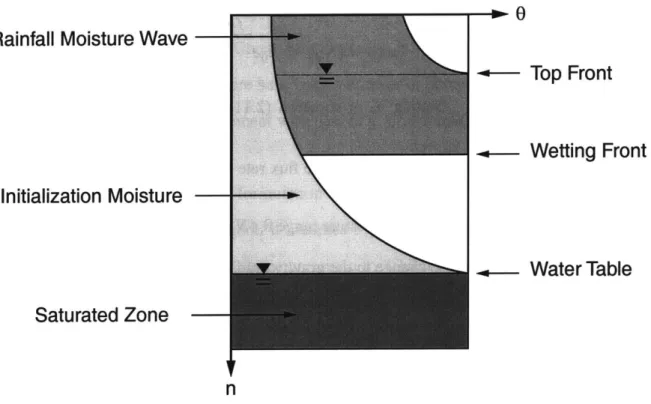
introduce some of the variables used in further analysis. Consider the schematic soil mois-ture profiles presented in Figure 2.2 and 2.3. There are two fronts depicted in figure 2.2: the wetting and the top front. As in the saturated infiltration case, the wetting front represents penetration of the moisture wave into the soil. It separates the infiltrated rainfall from the initial soil moisture profile in a discontinuous piston-like fashion as in the Green-Ampt model. The top front represents the ascent of the shock wave caused by the formation of the perched saturation zone. The normal depths to the wetting and the top front are correspond-ingly denoted as Nf and N,. They coincide if there is no perched layer and the soil column is therefore in the unsaturated state (Figure 2.3).

0

Rainfall Moisture Wave

Top Front

Wetting Front

Initialization Moisture

Saturated Zone

n

Figure 2.2: Schematic representation of the computational element vertical structure within the RIBS

The total moisture content above the wetting front Mt can be divided into an unsatur-ated area (from the land surface down to the top front) and a saturunsatur-ated area (between the top and the wetting front). The unsaturated moisture content Mt (attributed to the depths from

the land surface down to the top front) and the saturated moisture content M, (between the top front and the wetting front) can be expressed as:

N, _N

1

MU = fO(n)dn Ms = f0(n)dn M, = Mu+Ms (2.15)

0 _N,

If Nt= Nf , Mt is equal to Mu .

- Wetted wedge dynamics: No perched zone

One of the key assumptions made in the RIBS infiltration model is that while recog-nizing the importance of the capillary forces, gravity is considered to be the dominant com-ponent in the infiltration process. For the case when the perched zone has not formed yet, an expression for an equilibrium soil moisture profile corresponding to a constant rainfall intensity R can be derived (Cabral et al., 1992). The profile maintains a constant unsatur-ated conductivity (equation (2.9)) throughout the whole wetted thickness between the soil surface and the wetting front. This permits expressing the moisture content as a function of depth to the wetting front:

fn

0(R, n) = (Os -Or)e +Or, for 0 n Nf (2.16)

It is therefore assumed that irrespective of the suction effects at each point of the wetted wedge, the moisture profile quickly adjusts itself to the equilibrium profile. The assumption is reasonable provided that it is mostly applied to the top portion of the soil col-umn where higher conductivity due to macroporosity is the primary factor in soil moisture redistribution. This would also be plausible for initially wet soils in which capillary effects play a minor role.

In order to deal with variable rainfall rates and to account for the subsurface fluxes between the computational elements, Garrote [1993] made several additional assumptions. At all times moisture gets redistributed in the normal direction in order to attain an average

uniform normal flow. This implies that only a single moisture wave will propagate down-wards, regardless of the variability of rainfall intensity during the storm. This is a strong assumption which is, to some extent, supported by the unsaturated infiltration mechanism: local moisture accumulation increases the hydraulic conductivity and correspondingly increases the local normal flux, and hence moisture will tend to migrate from that point; conversely, if the moisture content is lowered, the conductivity becomes lower and water will tend to accumulate in that area. The implication is such that the flux variations in the normal direction are quickly smoothed out.

The solution adopted in the model is to define an "equivalent" rainfall rate Re (Gar-rote, 1993), a value that would lead to the same moisture content in the unsaturated portion of the pixel above the wetting front as from a constant rainfall at rate Re under equilibrium conditions. Therefore it is sufficient to know the amount of moisture and depth of the wet-ting/top front in order to get the Re. The moisture profile is given by equation (2.16). Inte-grating the moisture amount above the wetting front, substituting R with the "equivalent" rainfall rate Re and equating the expression to the unsaturated moisture content Mu:

N, - 1 fn

Mu

K~(Os-Or)e'

+Or

dn

(2.17)

0 On

one can solve for Re:

Mu

_-

OrN1

Re = Kn(O, n) = KO - (2.18)

f(s~r ~ )

where Kn(9, n) is a constant unsaturated hydraulic conductivity (by equation (2.9)) corre-sponding to the moisture amount Mu contained in the wetted wedge in the range of depths 0 to Nf.

The redistribution normal flux for the unsaturated wetted wedge that is discontinu-ous at the wetting front depth (Figure 2.3) is formulated by analogy with (2.14):

qn(Nf) = K,(Nf)coscc + TF,(Nf) (2.19)

where K,,(Nf ) is in fact Re since the wedge has constant unsaturated conductivity, and

',e(Nf) is the capillary drive across the wetting front in unsaturated conditions.

Physi-cally, the last term depends on the initial wetness of the soil profile as well as on the mois-ture magnitude in the wetted wedge. For the discontinuous profile, the range of moismois-ture values for which ie(Nf) has to be evaluated corresponds to [0e(Re, Nf), Oi(Nf)] where 0; (N) is the moisture content at the depth Nf of the initial moisture profile, and

0 (Re, Nf) is the moisture content obtained using equation (2.16) for Nf using Re instead of

R. Oe (Re, Nf) represents the maximum moisture value in the wetted wedge (Figure 2.3). Appendix 2 gives an approximation for the effective unsaturated capillary pressure

evalu-ated for an arbitrary moisture range in soils with decaying saturevalu-ated conductivity:

3 + 1 3+ +

S X(Nf) - Si .X(Nf)

hf(Nf, O, Oe) = tb 3X(Nf) e1 (2.20)

(0,( Re, Nf ) -0,.)

where Sei(Nf) is defined as previously and See(Nf) = (s - Or) If we now use

an unsaturated form of Darcy's law assumed by Smith et. al. [1993] (equation (26) of the paper), then the second term of (2.19) becomes:

hf(Nf, Oi,Oe)

Tie(N, Oi, 0e) = -Ksn(Nf) N (2.21)

tf

- Perched zone fonnation

Given that the saturated conductivity decreases with normal depth, the equivalent rainfall rate (defined in (2.18)) at some point may become equal to the saturated conductiv-ity at the depth of the wetting front N*:

Re = Ksn(N*) (2.22)

One can solve for the depth within the soil profile N*(Re) where saturation occurs:

N*(Re) = i n) (2.23)

According to the expression (2.16), N*(Re) represents the depth at which saturation devel-ops. If the moisture influx above the wetting front is high enough, water accumulates above that level and perched saturation develops (Figure 2.3 and 2.2). The top front represents ascent of the moisture wave propagating upwards from the depth N*(Re).

Os

i Io 0

Nt= Nf

N*

--

Top

/

Wetting Front

+-- Saturation Level

n

Between the wetting front and the top front the soil column is saturated (Figure 2.2). Using similar assumptions as for the ponding case, we write an analogous expression for the normal flux:

qn(Nf, N) = Keff(Nf, N,)cosa +'' i,(Nf) (2.24)

where Kfg is as previously the harmonic mean of the conductivities over the saturated thick-ness:

Kef (Nf, N,) = K0 f (Nf N, (2.25)

e -e

and Tis (Nf) uses the same suction head formulation as in (2.13).

- Evolution offronts

Other simplifications in RIBS are based on the idea of decoupling the vertical and horizon-tal moisture equations. The one-dimensional model of infiltration, when applied to a bounded domain, such as a regular grid element, produces a net flow of moisture at the downslope boundary which is transmitted to a contiguous element. Decoupling of the equa-tions allows one to consider the imbalance between the subsurface influxes and outfluxes as a component of the total moisture balance of the pixel above the wetting/top front. All moisture coming from the zone located above the ground water level of upstream cells and leaving the unsaturated/perched saturated zone of the current element is considered as a part of equivalent rainfall Re and participates in the water balance above the wetted wedge.

The three state variables, the moisture content, the top front, and the wetting front depth, define the status of the wetted wedge in the soil column. Below the wetting front the moisture profile corresponds to the initial pre-storm distribution and is given analytically as a function of depth to the water table. The accumulated amount of water in a pixel is esti-mated from a balance equation and is updated during each time step. Adding the accumu-lated value to the initial moisture content above the wetting front gives the value of M,. For

the unsaturated state (Figure 2.4), the wetting front evolution is described by a first-order differential equation (Cabral et al., 1992; Garrote, 1993) in the form:

dN = qn(Nf)

- (2.26)

dt Oe(Re, Nf) - Oi(Nf)

where qn is the redistribution flux value defined in (2.19), 0, (N) and Oe(Re, Nf) are the mois-ture contents also introduced previously. Equation (2.26) is approximated by the backward in time finite-difference:

t t-1 t-1

At O(R ,N(-f)-O;(N)- (2.27)

where index "t" defines the time level, and At is the computational time step.

The dynamics of the wetting front for the perched saturated and the surface satu-rated state (Figure 2.4) are defined as:

dNf qn(Nf, N,)

(2.28)

dt OS - 0(Nf)

which is numerically approximated in the same fashion as (2.27).

In the modified RIBS, evolution of the top front in the perched saturated state is dif-ferent from the formulation used by Garrote [1993]. The original formulation assumes a discontinuity in the moisture content at the top front: from the land surface the profile fol-lows the distribution corresponding to N*(Re), the depth at which perched saturation started developing, and abruptly becomes 0, at the top front (see Garrote, 1993 for details). This introduces certain difficulties since the moisture profile above the top front can not be easily treated with arbitrary upper boundary flux conditions, e.g. handling the moisture profile during the periods of rainfall hiatus or interstorm periods. Instead, it was assumed that the top front at each time t represents the saturation depth corresponding to some Re . Accord-ing to (2.23):

N, = N*(R') = In [ (2.29)

.-Re-where Rt is the corresponding "equivalent" rate which leads to saturation at Nt (Figure 2.2). The moisture balance equation can be used to define the top front position once the flux value q,(Nf, Nt) at the wetting front is known. A simple analytical expression in closed form can be derived (Appendix 3) for the top front evolution:

t t-1 E ~

(B-N _{-Nt =-LambertW}

[ e s] _{B (2.30)}

t-1I t-1I t fN'~-1

B -At [n( Nf , N, ) - R tot] 6 e C

where Rtor is the total net moisture influx/outflux for the pixel which may include rainfall, the net lateral subsurface moisture exchange, and evapotranspiration and is based on the idea of decoupling the vertical and horizontal moisture equations. LambertW(z) is the Lam-bert function defined as the root of the equation: W(z)e = z . A general description

of the function is given by Corless et al. [1996]. Effective numerical algorithms evaluating the function to a desired precision have been developed (Corless et al., 1996). The RIBS implementation code has an added function-member estimating the Lambert function.

The expression (2.30) allows for updating N, and conveniently handles the soil moisture profile above the perched saturation zone under arbitrary flux conditions. If the top front reaches the soil surface, N, is assigned to zero. In contrast, during interstorm con-ditions the soil moisture can get redistributed such that the perched saturation zone will van-ish. In this case, the unsaturated wedge will form and the above expression is not applicable anymore. A more detailed description of how sequences of storm and interstorm conditions are handled in the model given in Section 2.2.

-Subsurface flow exchange

Terrain slope, heterogeneity, and anisotropy produce a diversion of infiltration from the ver-tical and thus a lateral movement of moisture may exist. Once the values of the state vari-ables are known the horizontal moisture outflow from the cell can be evaluated. A