Control of a simulated, three-dimensional bipedal robot to initiate walking, continue walking, rock side-to-side, and balance

(1)

Control of a Simulated, Three-Dimensional Bipedal Robot to

Initiate Walking, Continue Walking, Rock Side-to-Side, and

Balance

By

Allen S. Parseghian

B.S., Electrical Engineering and Computer Sciences (1998) University of California, Berkeley

Submitted to the Department of Electrical Engineering and Computer Science in partial fulfillment of the requirements for the degree of

Master of Science in Electrical Engineering and Computer Science at the

MASSACHUSETTS INSTITUTE OF TECHNOLOGY September 2000

©

A uthor ...

Department of Electrical Engineerng and Computer Science August 4, 2000

C ertified by ...

Gill A. Pratt Assistant Professor ofEkctrical Engineering and Computer Science

Thesis Supervisor

Accepted by ...

Arthur C. Smith Chairman, Department Committee on Graduate Students

MASSACHUSETTS INSTITUTE OF TECHNOLOGY

(2)

Control of a Simulated, three-dimensional Bipedal Robot to initiate

walking, continue walking, rock side-to-side, and balance.

By

Allen S. Parseghian

Submitted to the Department of Electrical Engineering and Computer Science On August 4, 2000, in partial fulfillment of the

requirements for the degree of

Master of Science in Electrical Engineering and Computer Science

Abstract

Physical-based control using center of mass, center of pressure, and foot placement is used to enable a simulated twelve-degree of freedom, seven-link, three-dimensional bipedal robot to lean sideways, pick up its foot and start walking on a flat surface.

Energy analysis is used to compel the same simulated robot to do a side-to-side rocking motion and eventually come to a stop. If the robot is pushed hard enough, it will raise its leg that is in the air in the frontal plane to prevent itself from falling.

Center of mass and center of pressure analysis is used to enable the same robot to balance on one foot and stand.

Thesis Supervisor: Gill A. Pratt

(3)

Acknowledgments

I thank my adviser, Gill A. Pratt for allowing me to explore the idea of 3D walking. Thanks to all the members of the Leglab for all their tremendous support and advice.

I would like to thank all the friends I made over these years. Thanks to Jerry Pratt and Peter Dilworth for walking control advises. Thanks to Daniel Paluska for teaching me how to use our in-house software package, Creature Library. Thanks to Ben Krupp for helping me set up the software for M2. Thanks to Chris Morse for answering my questions regarding robot hardware. Thanks to John and Chee-Meng for discussing their walking algorithms with me. Thanks to Andreas for going out of his way trying to improve the M2 software environment.

I'd like to dedicate this thesis to my parents and my sister for their unbelievable support throughout my school years and believing in me.

This research was supported in part by the Defense Advanced Research Projects Agency under contract number N39998-00-C-0656 and the National Science Foundation under contract numbers IBN-9873478 and 1S-9733740.

(4)

(5)

List of Figures

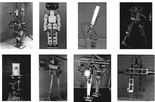
1-1 Some bipedal robots. From left to right: WL-10RV1 from Waseda, P2 from Honda, Toddler from UNH, the Moscow State University Biped, SD-2 from Clemson and Ohio State, Biper from University of Tokyo, Meltran II from Mechanical Engineering Lab in Tsukuba, and Timmy from Harvard. 1-2 Diagram illustrating the general control technique used in this thesis.

2-1 M2, the three-dimensional bipedal robot has three degrees of freedom at each hip, one degree of freedom at each knee, and two degrees of freedom at each ankle. 2-2 A rectangular foot has been used for M2.

2-3 Cylindrical shins have been used on M2. 2-4 The body of M2 has a semi-ellipsoidal shape. 2-5 Cross-section of the body of M2.

2-6 Ankle joint of M2 has two degrees of freedoms, roll and pitch. 2-7 Knee joint of M2.

2-8 Each hip joint of M2 has three degrees of freedoms, roll, pitch and yaw. 2-9 Model of a leg of M2 showing all the degrees of freedoms.

3-1 Virtual spring is used at M2's ankle pitch joint. 3-2 Knee strop is used to prevent the knee from inverting.

3-3 As the thigh of the robot is swung forward, due to natural dynamics of the biped, the shin too swings which causes the knee to straighten.

4-1 Finite state machine is used for walking initiation. 4-2 Robot is leaning to the side in state 1.

4-3 Robot is picking up its foot in state 2.

4-4 The whole walking initiation process is displayed in two different angles.

4-5 Geometric drawing of M2 in z-x plane. 4-6 Geometric drawing of M2 in the z-y plane.

4-7 Finite state machine with eight states is used to perform the walking algorithm. 4-8 Initiation of state 0. 4-9 Initiation of state 1. 4-10 Initiation of state 2. 4-11 Initiation of state 3. 4-12 Initiation of state 4. 4-13 Initiation of state 5. 4-14 Initiation of state 6. 4-15 Initiation of state 7.

(7)

4-18 Forward/sideways velocities and position of center of mass of M while it is walking.

4-19 Position of M2 joints while it is walking. 4-20 Torques at the M2 joints while it is walking.

4-21 External forces were applied on the robot when it was in this configuration.

4-22 Forward velocity of the robot when an external force in the positive X direction was applied.

4-23 Position of the center of mass of the robot measured from a fixed point when an external force in the positive Y direction was applied.

4-24 Position of the center of mass of the robot measured from a fixed point when an external force in the positive Y direction was applied.

4-25 Forward velocity of the robot when an external force in the positive X, Y, and Z directions were applied.

4-26 Position of the center of mass of the robot measured from a fixed point when an external force in the positive X, Y, and Z directions were applied.

4-27 M2 kicking its leg out in order to balance.

4-28 M2 is modeled as an inverted pendulum, which can rotate about its support ankle. 4-29 Finite State Machine with six states is used to achieve the side-to-side rocking

motion.

4-30 M2 is descending when the left foot is the support foot. 4-31 M2 is in double-support state after descending from left. 4-32 M2 is ascending when the right foot is the support foot. 4-33 The whole side-to-side rocking process is displayed. 4-34 M2 balancing on one foot.

(8)

List of Tables

2-1 Feet specification of M2.

2-2 Shins specifications of M2. 2-3 Body specifications of M2.

4-1 Control parameters of body roll in state 0. 4-2 Control parameters of body pitch in state 0. 4-3 Control parameters of body yaw in state 0. 4-4 Control parameters of left knee in state 0. 4-5 Control parameters of left ankle roll in state 0. 4-6 Control parameters of left ankle pitch in state 0. 4-7 Control parameters of right hip pitch in state 0. 4-8 Control parameters of right ankle roll in state 0. 4-9 Control parameters of right ankle pitch in state 0. 4-10 Control parameters of body roll in state 1.

4-11 Control parameters of body pitch in state 1. 4-12 Control parameters of body yaw in state 1. 4-13 Control parameters of left knee in state 1. 4-14 Control parameters of left ankle roll in state 1. 4-15 Control parameters of right hip pitch in state 0.

4-16 Control parameters of body roll in state 2 before foot strike. 4-17 Control parameters of body pitch in state 2 before foot strike. 4-18 Control parameters of body yaw in state 2 before foot strike. 4-19 Control parameters of left knee in state 2 before foot strike. 4-20 Control parameters of left ankle roll in state 2 before foot strike. 4-21 Control parameters of right hip pitch in state 2 before foot strike. 4-22 Control parameters of right knee in state 2 before foot strike. 4-23 Control parameters of right ankle pitch in state 2 before foot strike. 4-24 Control parameters of body roll in state 2 after foot strike.

4-25 Control parameters of left ankle pitch in state 2 after foot strike. 4-26 Control parameters of right knee in state 2 after foot strike. 4-27 Control parameters of right ankle roll in state 2 after foot strike. 4-28 Control parameters of right ankle pitch in state 2 after foot strike. 4-29 Control parameters of body roll in state 3.

4-30 Control parameters of body pitch in state 3. 4-31 Control parameters of body yaw in state 3. 4-32 Control parameters of right knee in state 3.

(9)

4-34 Control parameters of left hip pitch in state 3.

4-35 Control parameters of left knee in state 3. 4-36 Control parameters of left ankle roll in state 3. 4-37 Control parameters of left ankle pitch in state 3.

(10)

Chapter 1 Introduction

Proving the stability of certain systems using the present control techniques could be a very painstaking process, if not impossible. Dynamically walking two-legged robots are systems that belong to this category which are highly nonlinear and naturally unstable so that legged locomotion researchers are yet to come up with a convincing, mathematically based control system that can fully explain why a biped is able to walk or fail to walk continuously. Bipeds are multi-input, multi-output systems that are both continuous and discrete. While in single support, the system operates in a continuous fashion, as soon as the support leg switches, there is discreteness, as well.

In order to reduce the complexity of the bipedal robotics systems, most researchers have only settled for building/simulating planar bipeds i.e. bipeds that can only walk forward or backward in the sagittal plane. These kinds of bipeds lack the roll and the yaw degrees of freedoms that would allow them to operate in the three-dimensional space, therefore these types of robots have to be connected to an external stationary device such as a boom in order to be contained in a plane. Simulation is an extremely useful tool to explore a control system for a bipedal robot, especially if it has all the necessary degrees of freedom in order for it to be able to walk in the three-dimensional world. Great design of a biped can contribute significantly to a successful bipedal locomotion. In this thesis, mostly physical intuition will be used to control a simulated three-dimensional bipedal robot to walk, rock side-to-side, balance on one leg, and stand on both legs.

1.1 Background

Many researchers have studied legged locomotion by simulating, building, and controlling walking, hopping, and running robots. Simple controllers can be used and natural dynamics can be exploited to enable bipedal robots to perform complicated tasks such as walking ([14], [15], [16], [17], [18]). There have been quite many passive walking robots/toys built such that they completely rely on their natural dynamics and the gravitational force in order to be able to operate. McGeer explored passive walking and showed that a system that has no sensors, actuators, or any sort of a brain can walk downhill, if appropriate hardware geometry is used ([12]). Jessica Hodgins [8] has too

(11)

these passive walkers is that it is easy to build them and also they do not require actuators, sensors, or computers in order to make them move, but these robots have limited capabilities such as they cannot walk up a slope.

Pratt et al. [17] used a technique called "Virtual Model Control" to enable their planar biped, Spring Flamingo to walk. This technique employs virtual springs and dampers to describe interactive force behavior. The robot behaves as if those components were in fact attached to it. The virtual components exert virtual forces, which are transformed into real torques at the joints of the robot via Jacobian transformation matrix. The advantage to this technique is that the controller is mostly intuitive and easy to understand.

There have also been quite many robots built that are fully power-operated without use of natural dynamics ([2], [7]). One of the advantages to these types of robots is that they have wide range of capabilities such as walking on a rough terrain, but these robots can have unnatural looking motions due to limitations in their actuators. Also the control of these types of robots can become quite complicated especially if the controller requires an exact dynamic model of the system. Controlling a fully powered three-dimensional biped that is fully dependent upon its dynamic model is quite a complicated task because it requires extremely complicated dynamics equations of motion in order to describe its motion.

There have been robots such that their control is based on their certain joints and/or certain points on their structure track pre-specified trajectories ([4], [6], [7], [9]). One of the advantages to this approach is that the controller is relatively simple since all the trajectories are known, but if there is a slight change in the shape of the robot or the terrain on which the robot walks, the controller may not work any longer and it will usually require supplemental control in addition to trajectory tracking.

Kun et al. [11] used CMAC neural networks to control the lateral (sideways) lean angle, hip motion in the sagittal plane, and lateral roll of the ankles while the robot is in double support. One of the advantages of employing neural networks in biped control is that it will most likely result in a motion, which is fairly close to the desired one. One disadvantage is that it might take the robot several iterations until the goal is achieved. Yamaguchi et al. [9] employed a heavy trunk with 2 degrees of freedom to ensure dynamically that the Zero Moment Point (ZMP) of the robot stayed within the polygon of the support foot. One advantage to this approach is that it will give us an extra link, which can contribute to controlling the robot successfully, but at the same time it might cause a very unnatural looking motion. The other disadvantage is that it will increase the weight of the robot.

Many dynamically and statically stable bipeds have been built and controlled, but the only robots that have been built which resemble the structure of an adult human closer than any other biped is the Honda company biped robots, P2 and P3 ([7]). P3 can perform several complicated tasks such as walking on a flat ground, turning, walking

(12)

up/down stairs, balancing, and pushing objects around all in three-dimensional space without being held by any external devices such as a boom.

Figure 1-1 shows pictures of some previously powered bipedal robots.

Figure 1-1: Some bipedal robots. From left to right: WL-10RV1 from Waseda, P2 from Honda, Toddler from UNH, the Moscow State University Biped, SD-2 from Clemson and Ohio State, Biper from University of Tokyo, Meltran 11 from Mechanical Engineering Lab in Tsukuba, and Timmy from Harvard.

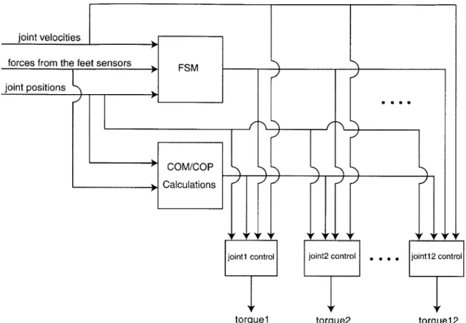
The control method described in this thesis differs from the others in that it is very simple to understand, it does not require dynamic calculations of the robot, it calculates the position of the center of mass and center of pressure of the robot at every instance in such a way that couplings between joints are taken into account. Each joint, triggered by finite state machine conditions, is servoed independent from the others therefore making the control more intuitive. Position of the center of mass and center of pressure of the robot are controlled using ankles, therefore every time the ankles are servoed, the couplings between all the joint of the robot are taken into account. A simple sideways foot placement control is used which is a function of sideways velocity of the center of mass of the robot and the sideways displacement of the position of the center of mass of the robot's body with respect to the support foot. Natural dynamics is exploited to simplify

(13)

the sagittal (forward / backward) plane control. A block diagram describing the control strategy in this thesis is shown in Figure 1-2.

joint velocities

forces from the feet sensors joint positions FSM COM/COP Calculations

K

jointi control torquel

K

I

joint2 control torque2 0 * * *

K

jointl2 control torque12

Figure 1-2: Diagram illustrating the general control technique used in this thesis.

1.2 Thesis Contents

This thesis is organized as follows: Chapter 2 describes model of the robot

Chapter 3 describes natural dynamics of the robot

Chapter 4 describes the simulation algorithms for walking initiation, walking continuation, balancing on one foot, standing

Chapter 5 conclusions and future work

K

(14)

(15)

Chapter 2 Robot Model

2.1 Model background

The simulation model of this robot is based on the actual hardware design of the MIT Leglab biped, M2. The previous version of the Leglab biped, Spring Flaming, was a planar robot with a total of six degrees of freedom, one joint at each hip, one at each knee, and one at each ankle. The robot was connected to a boom in order to prevent the biped from falling side-to-side. The newer generation of the Leglab biped, M2, is supposed to be able to walk freely without being held by any external devices.

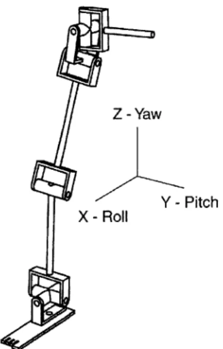
roll, pitch, yaw

pitch

roll, pitch

Figure 2-1: M2, the three-dimensional bipedal robot has three degrees of freedom at each hip, one degree of freedom at each knee, and two degrees of freedom at each ankle.

(16)

For many years, the tradition in the Leglab has been so that every robot is simulated and controlled first, where the simulation model is created based on the specifications of the actual hardware of the robot before the control code is tested on the actual hardware. Figure 2-1 shows the simulation cartoon model of this biped. As it can be seen it this figure, there are three degrees of freedom at each hip (roll, pitch, and yaw), one degree of freedom at each knee (pitch), and two degrees of freedom at each ankle (roll, pitch) for a total of twelve degrees of freedom. This three-dimensional seven-link biped possesses all the degrees of freedoms required in order to freely traverse in the three-dimensional world, including turning.

2.2 Links Specifications

The specifications of each link (mass, length, height, and width) are chosen to match an average male adult human, especially those of the designer's (Daniel Paluska).

2.2.1 Feet

The biped model has 2 rectangular feet as shown in Figure 2-2 with the specifications shown in Table 2-1.

Mass (kg) Length (m) IWidth (m) Height (m) Ankle to Toe (m) Ankle to Heel (m)

0.562 0.203 0.0889 0.0641 0.152 0.051

Table 2-1: Feet specification of M2.

Height

Figure 2-2: A rectangular foot has been used for M2.

(17)

The contribution of the feet in natural-looking walking is extremely critical, for instance, if the feet are designed to be too wide, it might result in a very unnatural-looking landing of the foot. Obviously, feet cannot be too narrow either since the side-to-side control would become very challenging. Feet cannot be too long either since foot clearance in the swing phase would be a difficult task to achieve. Feet also play a major role in the toe-off state, where the robot's back-foot pushes against the ground in order for the robot to move forward and go into its opposite single support state, therefore if the feet are too narrowly designed, this task may not be completed successfully as the robot's feet can easily be twisted. The original design of the hardware of the foot included toes as well which was a triangular piece attached to the front of the foot. Since we were uncertain about the stability issues of the robot with toes, we decided to stick with simple rectangular feet.

2.2.2 Shins

The biped has two cylindrical shins as shown in Figure 2-3 that at the lower end are connected to the feet to form the ankle joints. The shin specifications are listed in Table

2-2.

Mass (kg) Length (mn) Radius (in) 2.72 0. 4321 0.05 1

Table 2-2: Shins specifications of M2.

Figure 2-3: Cylindrical shins have been used on M2.

On the hardware of the robot, carbon fiber tubes are used to keep the weight as low as possible. Two actuators are attached on each shin to servo each ankle. With the actuators mounted, each shin weighs about 2.7 kg.

(18)

2.2.3 Thighs

Thighs are exactly similar to the shins. At the lower end, each thigh link is connected to the upper end of the appropriate shin to form the knee joints.

2.2.4 Body

The body has too parts. The lower part of the body consists of a short cylinder as shown in Figure 2-4 and the upper part of the body which is connected right on top of its lower part is a semi-ellipsoid. The body specifications are shown in Table 2-3.

Mass (kg) Cylinder Height (m) Cylinder Radius (m) Semi-Ellipsoid Height (m)

12.71 0.05081 0.2281 0.45721

Table 2-3: Body specifications of M2.

---74 L~I ,' Cylinder Height U I I-' Cylinder Diameter

Figure 2-4: The body of M2 has a semi-ellipsoidal shape.

The upper ends of the thighs are connected The length of the body is critical in stable control since gravity can easily tip it over.

at the two hip joints shown in Figure 2-5. control i.e. a taller body is challenging to

Semi-Ellipsoid Height

(19)

Hip Spacing

Cross-Sectional Diameter

Figure 2-5: Cross-section of the body of M2.

2.3 Joint Characteristics

2.3.1 Ankles

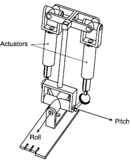
Each ankle has two degrees of freedom (roll and pitch). A universal joint has been used to form this joint. The pitch degree of freedom allows the robot to move its feet up and down, while the roll degree of freedom allows the robot to move its feet side-to-side. Although ankle roll is not necessary in 3D walking if hip roll joint is present, but its availability allows the robot's feet to stay flat on the ground during almost throughout the entire single support phase. Ankle roll can too contribute to the control of the biped such that it will not fall sideways while walking. At each ankle pitch, it is assumed that a virtual spring is attached between the foot and the shin which enables the robot's heel to come off the ground naturally as its weight is transferred forward. A more detailed explanation on virtual spring of the ankle pitch will be given in chapter 3 of the thesis. Figure 2-6 shows how each ankle pitch of the actual hardware is constructed. The two actuators attached on each shin servo the ankle pitch and roll. If only ankle pitch torque is desired, they both output equal forces in the same directions, and if only ankle roll torque is desired, they both output equal forces but in opposite directions. If both ankle pitch and roll torques are desired, the forces are related in a more complicated way which is outside the context of this thesis since the simulation uses a model such that for every joint there is a motor directly servoing it.

(20)

Actuators

Pitch Roll

Figure 2-6: Ankle joint of M2 has two degrees of freedoms, roll and pitch.

2.3.2 Knees

Each knee has one degree of freedom (pitch), which is made of a pin joint (Figure 2-7). Just like the case in the humans, the knee is limited by a stop that does not allow the shin to bend out where out is defined the direction in which the swing shin is rotating up. Therefore a knee stop is used in the simulation model in order for us to be able to lock the knees as soon as the leg is straightened during landing and support phases.

Pitch

(21)

2.3.3 Hips

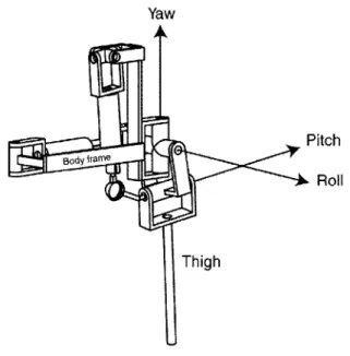
Each hip has three degrees of freedom (roll, pitch, and yaw). There is a universal joint used for the roll and the yaw degrees of freedom, and a pin joint for the pitch degree of freedom, which is based on the design of the actual hardware as shown in Figure 2-8.

Yaw

Pitch

Body irame

Roll

Thigh

Figure 2-8: Each hip joint of M2 has three degrees of freedoms, roll, pitch and yaw.

The pitch degree of freedom allows the robot to swing its leg forward and backward, the roll degree of freedom provides the side-to-side motion of the leg which the robot needs in order to place its foot where it can prevent itself from falling sideways, and the yaw degree of freedom is the twist which is required for the robot to be able to turn.

2.4 Summery

The robot model has seven links and twelve degrees of freedom, which allows the biped to traverse in the 3D world. There are three degrees of freedom on each hip, one degree of freedom on each knee, and two degrees of freedom on each ankle. This biped is meant to have all necessary degrees of freedom in order to walk as naturally as possible without being held by an external object. Figure 2-9 shows a drawing model of the robot's leg with all the degrees of freedom.

(22)

0

Z -Yaw

Y -Pitch

X -Roll

(23)

Chapter 3 Robot's Natural Dynamics

Many researchers such as McGeer [12], Goswami et al [5], and Garcia et al [3] have exploited natural dynamics to make their walking machines walk passively meaning that their machines rely completely on their natural dynamics and gravitational force in order to traverse along. Powerful design of a robot can simplify the control significantly by making use of natural dynamics. For instance, spinning an object about its small and large axis is naturally stable and requires no complicated control system. Pratt et al have employed natural dynamics in order to make a powered planar bipedal robot walk. They have also shown that natural dynamics can simplify control of a powered planar biped significantly.

In this chapter, the idea of natural dynamics is extended to the three-dimensional simulated bipedal robot, M2. First, the natural dynamics mechanisms will be explained and later in chapter 4, they will be exploited in order to control M2.

3.1 Springy Ankle

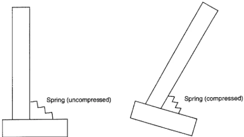
The ankle of the hardware of M2 contains a rubber stop that serves as an ankle limit, which enables the robot's heel to come off the ground passively as the robot's center of mass is moving forward. In the simulation model of M2, a virtual quadratic spring is used in order to serve this purpose. Figure 3-1 illustrates how a compliant ankle helps the heel to come off the ground. As the robot's center of mass is moving forward, the spring gets compressed, the center of pressure moves to the toes, as a result of that the heel lifts off the ground. Combination of springy ankle and active control will allow the robot's toe to come off the ground. As soon as the heel of the robot lifts off, the ankle pitch is servoed to open up, as a result of that the toes push off against the ground, which helps the robot to go into toe-off state. There are of course differences between a rubber stop and model of the spring used in the simulation, therefore appropriate adjustments need to be made for the robot's heel to lift off at the right time. A late lift off can cause the robot to not get over its apex, and an early lift or a hard push can cause the body roll to go unstable.

(24)

Spring (uncompressed) Spring (compressed)

Figure 3-1: Virtual spring is used at M2's ankle pitch joint.

3.2 Knee Stop

Walking with a straightened support knee is simpler to control since the robot can be modeled as an inverted pendulum. A knee stop is used so that during walking, every time the knee is straightened right before touchdown or during support, the knee is servoed to a locked position, which creates a reliable and strong support leg. Figure 3-2 illustrates the knee stop. On the hardware of the robot, rubber-stop are used so that when the knee is straightened, there will be soft contact between the shin and the thigh, where in the simulation, damping is used right before the swing leg is straightened so that the shin will not bang into the knee stop too violently. As soon as the knee is straightened, stiff

proportional gain is used to ensure the knee is locked.

Thigh

Rubber-stops

(25)

3.3 Passive Swing

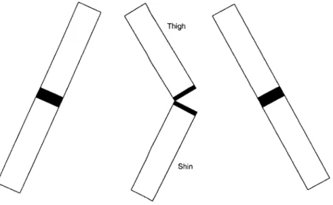
In the swing phase, Pratt et al. [15] showed that the shin can swing passively while the swing hip pitch is servoed forward. This makes the control easier in a sense that the active torque on the swing knee can be turned off and let the natural dynamics of the swing shin take over. Figure 3- 3 illustrates how the shin is swung forward. As soon as the knee is straightened, it is locked against its stop to maintain its straightened shape.

Thigh

Shin

Figure 3- 3: As the thigh of the robot is swung forward, due to natural the biped, the shin too swings which causes the knee to straighten.

(26)

(27)

Chapter 4 Robot Control

4.1 Simulation Algorithm For Walking Initiation

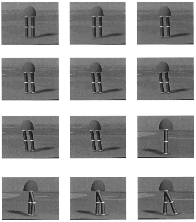
A Finite State Machine (FSM), comprising two states, is used for walking initiation control algorithm as shown in Figure 4-1. In the first state (Leaning Sideways), the robot uses one of its ankle rolls joints (in this case, the right one) to push against the ground (by twisting the right foot) and as a result of that, the robot leans to the opposite side. During the whole time that the robot is in state 1, all its joints are controlled using proportional-derivative controller. The body is controlled to have an upright position by servoing the hips while both of its legs are leaning sideways as show in Figure 4-2. The knees are in the locked position the whole time. The robot keeps pushing against the ground in the frontal plane until the position of its center of mass, which is measured from the left ankle falls on top of its left foot. This is when the biped goes into state 2 (Pick up Foot).

Leaning FoPikp()Walking

Foot icku (2)Finite State

Machine

Figure 4-1: Finite state machine is used for walking initiation.

In state 2 (Figure 4-3), most of the robot's weight has been taken off of its right foot, which makes it plausible for the robot to pick it up by driving its right hip pitch joint to a desired position. The knee joint of the right leg is bent at the same time while the left

(28)

knee maintains its locked position. The right foot is controlled to stay parallel with the ground to ensure foot clearance. Left ankle pitch is servoed to maintain the center of mass of the robot at a desired position in the sagittal plane so that the robot will not fall forward or backward. Left ankle roll is used to control the position of the center of mass of the robot in the frontal plane so that it won't fall to the side. As soon as the position of the right hip pitch joint reaches a certain threshold, the robot goes into a different state, which is when it starts walking.

Figure 4-2: Robot is leaning to the side in state 1.

(29)

Figure 4-4: The whole walking initiation process is displayed in two different angles.

4.2 Walking Continuation

(30)

The location of the center of mass of the robot is calculated in both frontal and sagittal planes and later used in the walking control algorithm.

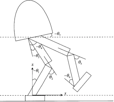
For the calculations in the sagittal plane (x-z), consider Figure 4-5.

-07

-04

-03

Z 05

02 -6

Figure 4-5: Geometric drawing of M2 in x-z plane. where 1= qja_ pitch 02 =qk 03 =qh_ pitch 04 = qrh_ pitch 05 = q _rk 06 = q ra _ pitch 07 = q _ pitch

xi is the position of the center of mass of link i in the x-z plane measured with respect to

the x-z reference frame located at ankle joint as shown in Figure 4-5. When the left foot is the support foot, x, _ L is used and when the right foot is the support foot, x. _ R is

(31)

The links are defined as follows:

i = 1 represents the left foot

i = 2 represents the left shin

i = 3 represents the left thigh

i = 4 represents the body

i = 5 represents the right thigh

i = 6 represents the right shin

i = 7 represents the right foot

the expressions for x _ L for i=1,2,3,4,5,6, and 7 are:

x₁ L =FOOT _ FORWARD -0.5FOOT _ LENGTH

x2 _ L -(0.5)(0.5)L _ SL _ L _x sin(q _la _ pitch)

x3 L =2x2 _L -(0.5)(0.5)L _ SL _ L _xsin(q _la _ pitch + q lk)

x4 L =2x2 L-0.5L SL_ Lxsin(qla pitch+qlk

)-CG _ Z _ OFFSET cos(q - roll) sin(q - pitch)

X5 L 2x2 L-0.5L SL_ Lxsin(qla pitch+qjk

)-(0.5)(0.5)L_ SLR_xsin(q pitch +qrh_ pitch)

x₆ L =2x2 L-0.5L_ SL_ Lxsin(qla_ pitch+ qjk)

-(0.5)(0.5)L _ SL _ R _ x sin(q - pitch + q - rh - pitch) -(0.5)(0.5)L _ SL _ R _x sin(q - pitch + q - rh - pitch + q - rk)

x7 L 2x_ L -0.5L SL_ Lxsin(qla pitch+qjk

)-(0.5)(0.5)L _ SL _ R _x sin(q - pitch + q _rh - pitch)

-(0.5)L _ SL _ R _x sin(q _ pitch+ q _rh pitch+ q _ rk )+

x, L cos(q - pitch + q -rh - pitch + q -rk + q - ra - pitch)

where

L _SL_ L _x = 2SHIN _ LENGTH cos(q - roll + q _lh _roll)

which is the length of the projection of the support leg onto the x-axis in the x-z plane when the left leg is the support leg.

and

L _SL _ R _x = 2SHN _ LENGTH cos(q _roll + q _rh _roll)

which is the length of the projection of the support leg on the x-axis in the x-z plane when the right leg is the support leg.

(32)

x₁ _ R = FOOT _ FORWARD -0.5FOOT _ LENGTH

x2 - R = -(0.5)(0.5)L _ SL _ R _x sin(q _ra _ pitch)

x3 _R = 2x2 _R -(0.5)(0.5)L SL_ R_xsin(q ra pitch+ qrk)

x₄ R = 2x₂ R 0.5L_ SL_ Rxsin(qra pitch+ q rk)

-CG _ Z _OFFSET cos(q - roll) sin(q - pitch)

x _ R = 2x₂_R -0.5L SLRxsin(q ra pitch+ q rk)

-(0.5)(0.5)L _ SL _ L _x sin(q - pitch + q - lh _ pitch)

x₆_R=2x₂_R 0.5L_ SLRxsin(q ra _pitch+ q rk)

-(0.5)(0.5)L _ SL _ L _x sin(q - pitch + q - lh - pitch) -(0.5)(0.5)L _ SL _ L _x sin(q - pitch + q - lh - pitch + q - lk)

x7 R=2x2 _R-0.5L

SL_R-xsin(q-ra-pitch+q-rk)-(0.5)(0.5)L _ SL _ L _x sin(q - pitch + q - lh - pitch)

-(0.5)L _ SL _ L _x sin(q _ pitch+ q _lh _ pitch+ q _lk)+

x_ R cos(q - pitch + q -lh - pitch + q -lk + q -la - pitch)

For the calculations in the frontal plane (y-z), consider Figure 4-6 shown below:

- Y3

Y 2

z

Y1

Figure 4-6: Geometric drawing of M2 in the y-z plane.

(33)

y, = q la roll

y2 = q _lh _roll

y3 = q _rh _roll

y4= q _ra _ roll

y5 = q _roll

yi is the position of the center of mass of link

j

in the y-z plane measured with respect to the z-y reference frame located at the ankle joint as shown in Figure 4-6. When the left foot is the support foot, y. _ L is used and when the right foot is the support foot,

yi _ R is used.

The links are defined as follows:

j

= 1 represents the left shin

j

= 2 represents the left thigh

j

= 3 represents the body

j

= 4 represents the right thigh

j

= 5 represents the right shin

j

= 6 represents the right foot

the expressions for y 's for i =1,2,3,4,5, and 6 are Y L =-0.5L_ SHIN _ Lsin(q _roll +q _ lh _roll)

y2 L =2y _ L -0.5L _THIGH _ Lsin(q roll +q _lh _roll)

y₃ L= 2y1 _ L - L _THIGH _ Lsin(q _roll +q _lh

_roll)-0.5 HIP _ SPACING cos(q - roll) + CG _Z _ OFFSET cos(q _ pitch) sin(q _roll)

y₄ L =2y, _L - L _THIGH _ Lsin(q _roll+q _lh

roll)-HIP _ SPACING cos(q - roll) - 0.5L_T _ S _ R sin(q - roll + q _ rh - roll)

Y5 - L = - L - L THIGH _ Lsin(q - roll + q _lh _roll) - HIP _ SPACING cos(q - roll)

-(L_T _ S _ R +0.5LS _S _R)sin(q roll + qrh roll)

y6 L =2y1 _ L - L THIGH _ Lsin(q _roll +q _lh _roll) - HIP _SPACING cos(q _roll)-(L _T _ S _ R + L_ S _S _R)sin(q _roll +q _rh

_roll)-0.5FOOT_ HEIGHT sin(q _roll + q rh _roll + q _ra _ roll)

where

L _ SHIN _ L = SHIN _ LENGTH cos(q _ la _ pitch)

(34)

which are the lengths of the projections of the shin and thigh of the support leg on the y-axis in the y-z plane, if the left leg is the support leg, respectively.

and

L _T _ S _ R = SHIN _ LENGTH cos(q _ pitch + q _rh _ pitch)

LS _S _R = SHINLENGTH cos(qpitch+ q rh pitch+ q rk)

which are the lengths of the projections of the thigh and shin of the swing leg on the y-axis in the y-z plane, if the right leg is the sing leg, respectively.

Similarly

y1 R =-0.5L _SHIN _ R sin(q _roll +q _rh _roll)

y2 R =2y _ R -0.5L _THIGH _R sin(q _roll +q _rh _roll) y3 R =2y1 _ R - L _THIGH _ R sin(q _roll +q _rh _roll)+

0.5 HIP _ SPACING cos(q - roll) - CG - Z _ OFFSET cos(q - pitch) sin(q - roll) y4 R = 2y1 R - L _THIGH _ R sin(q _roll + q _ rh _roll )+

HIP _ SPACING cos(q - roll) + 0.5L _T _ S - L sin(q - roll + q - lh - roll)

Y_ R = - R - L _ THIGH - R sin(q - roll + q - rh - roll) + HIP _ SPACING cos(q - roll) +

(L_T _S _ RL+0.5L_ S _ S _L)sin(q roll +qlh roll)

Y_ R = 2y_,- R - L _THIGH - R sin(q - roll + q - rh - roll) + HIP _ SPACING cos(q - roll) + (L_T _S _ L -LS S L)sin(q roll +qlh roll )+

0.5FOOT _ HEIGHT sin(q _roll + q _lh _roll + q _la _roll)

where

L _ SHIN _ R = SHIN _ LENGTH cos(q _ra _ pitch)

L _THIGH _ R = SHIN _ LENGTH cos(q - pitch + q - rh - pitch)

which are the lengths of the projections of the shin and thigh of the support leg on the y-axis in the y-z plane, if the right leg is the support leg, respectively.

and

L _T _ S _ L = SHIN _ LENGTH cos(q - pitch + q - lh - pitch)

LS _S _ L = SHINLENGTH cos(q pitch+q lh pitch+q _ik)

which are the lengths of the projections of the thigh and shin of the swing leg on the y-axis in the y-z plane, if the left leg is the sing leg, respectively.

(35)

4.2.2 Simulation Algorithm

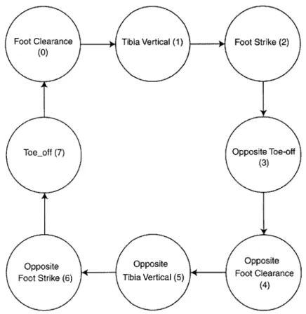
A finite state machine is used to perform the walking algorithm. The states are related as shown in Figure 4-7. A detailed control description of each joint in every state is explained below. All the positions of the joints have the form "q jointname". All the angular velocities of the joints have the form "qd jointname". All the desired positions of the joints have the form "q-d-joint-name". All the desired angular velocities of the joints have the form "qd-d-jointname"

Foot Clearance Tibia Vertical (1) Foot Strike (2)

(0)

Toe-off (7) Opposite Toe-off

(3)

Opposite Opposite Opposite

Foot Strike (6) Tibia Vertical (5) Foot Clearance

(4)

Figure 4-7: Finite state machine with eight states is used to perform the walking algorithm.

Foot Clearance

This state is initiated when the right ankle pitch exceeds a certain angle while pushing against the ground (Figure 4-8). The left leg is the support leg while the right leg is in the beginning of its swing phase. The control is as follows:

(36)

Figure 4-8: Initiation of state 0.

Body Roll: Body roll is controlled at the left hip roll by using both Proportional-Derivative (PD) and a feed forward term, which counters the effect of the gravitational force.

tau _lh roll =kroll(qroll -qd roll)+ b_ roll(qd- roll -qd _droll)+

(0.5(HIP _ SPACING) cos(q - roll) +

(CG - Z _OFFSET) sin(q - roll))(grav _

force

_body _roll _1)

where

HIPSPACING is the distance between the two

distance from the center of mass of the body to the

hip joints and CG_Z_OFFSET is the base of the ellipsoid.

Parameter Value

k roll 60

b roll 20

gravforce body rolI 225

q dLroll 0

gdad-roll 0

Table 4-1: Control parameters of body roll in state 0.

Body Pitch: Body pitch is controlled by servoing the left hip pitch joint using a PD controller such that it stays parallel to the ground. An offset is used to ensure upright

(37)

tau - lh - pitch = k _ pitch(q - pitch - q - d - pitch) + b _ pitch(qd - pitch - qd - d - pitch)

where Parameter Value kpitch 60 bpitch 20 _d_ pitch 0.1 qdadpitch 0

Table 4-2: Control parameters of body pitch in state 0.

Body Yaw: Body yaw is controlled by servoing the left hip yaw controller such that it maintains the least amount of twist.

tau -lh - yaw = k - yaw(q - yaw -q -d -yaw) +

b - yaw(qd - yaw - qd - d - yaw)

where Parameter Value kyaw 60 byaw 20 _d_ yaw 0 qd dcyaw 0 joint using a PD

Table 4-3: Control parameters of body yaw in state 0.

Left Knee: It is made sure that the left knee is servoed against its locked. This allows the robot to be like an inverted pendulum, easy transition from single support to double support.

stop so that it is tightly which will provide an

tau _lk = k _lk(q _d _1k - q _1k)+

b

- lk(qd -

d

-1k - qd-

1k)

where Parameter Value k/Ik 30 bIk 10 _djk 0 qcL dk 0

(38)

Left Ankle Roll: Position of the center of pressure is calculated from the left ankle. The desired position of the center of pressure is a function of the position of the center of mass error and sideways translational velocity of a point on the left hip joint.

L _com _err_ y = ycom_L+(frac oot width)(FOOT WIDTH)

L _cent_ press _ y _des = (b _ank _ yd)(lhip _ proj _ yd)+ (k _com _err _ y)(L _com _ err y) if (L cent _-press _ y _des > 0.5(FOOTWIDTH))

L _cent - press - y - des = 0.5(FOOT _WIDTH) if (Lcent_ press_ y _des < -0.5(FOOTWIDTH))

L _cent - press - y - des = -0.5(FOOT _WIDTH) tau _la _ roll=k _la _ roll _cop(Lcent press_ ydes - ycopL)

Parameter Value

k la roll cop 100

b ankyd -1

k comy 1

frac foot width 0.22

Table 4-5: Control parameters of left ankle roll in state 0.

Left Ankle Pitch: Velocity control is used velocity higher than a certain threshold.

to slow down the robot if it is moving with a

body - speed _ control - torque(vel)

double vel;

{

if (vel > vel _threshold)

return ( (vel _ gain)(vel2₎

else return (0)

}

A quadratic virtual spring is used to enable the robot's heel to come off the ground as the biped's weight is shifted forward.

double pass _ ank _ pitch _torque(pos, vel)

double pos, vel;

{

if ( pos < ank _ pitch _lim. set

return ((ank _ pitch - lim_ gain) (ank - pitch _ lim_ set - pos) 2

else return (0); }

(39)

tau - la - pitch = pass _ ank _ pitch - torque(q _la - pitch, qd - la - pitch) +

body - speed _ control _torque(x - vel)

where

x _ vel is the transnational velocity of the robot in the sagittal plane.

Parameter Value

vel threshold 0.91

veLgain 40

ank-pitchjlim set 0

ank-pitch-lim-gain 1000

Table 4-6: Control parameters of left ankle pitch in state 0.

Right Hip Pitch: Right hip pitch joint overshoot nor undershoot is achieved. too hard. An undershoot will result clearance.

is servoed to a desired position such that neither An overshoot can cause the robot's foot to land in a short swing which would mean no foot

tau _ rh _ pitch = k _ rh pitch(q _d _ rh _ pitch - q _ rh _ pitch)+ b _ rh pitch(qd _d drh _ pitch - qd _rh _ pitch)

where

q _d _ rh_ pitch = -q pitch+ qd rh _pitch_ final

Parameter Value

k_rhpitch 55

bjrhpitch 20

qgd_rhpitch final -0.5

qdcdu&rhpitch 0

Table 4-7: Control parameters of right hip pitch in state 0.

Right Knee: The right knee torque is completely shut down, therefore the shin of the swing leg is swung forward passively due to the servoing of the right hip pitch.

tau _rk =0

Right Ankle Roll: Right ankle roll is simply servoed to be held aligned with the shin of the swing leg.

(40)

tau _ra _ roll=k _ raroll(q _d _ ra _roll -qra_ roll)+ b _ ra roll(qd _ d _ ra roll - qd _ ra _ roll)

Parameter Value

k ra roll 4

b ra roll 1

qdLra roll 0

qdjdOra roll 0

Table 4-8: Control parameters of right ankle roll in state 0.

Right Ankle Pitch: Right ankle pitch is simply servoed to be pointing up the shin of the swing leg to ensure foot clearance.

tau _ ra _ pitch = k ra pitch(q _d _ra _ pitch - q _ra _ pitch)+

b ra pitch(qd _d _ra _ pitch - qd _ra _ pitch)

Parameter Value k-rapitch 7 bj rapitch 1 qgdjra-pitch -0.3 qddjra-pitch 0 with respect to

Table 4-9: Control parameters of right ankle pitch in state 0.

Tibia Vertical

This state is initiated when the left ankle pitch angle and right knee fall below a certain threshold (Figure 4-9). Most of the control in this state is similar to the control in the "foot clearance" state. If there are any differences in their parameters, they are shown in new tables.

(41)

Body Roll: Similar control to the "Foot Clearance" state.

Parameter Value

k roll 60

b rofl 10

gray force body roll_ 230

qd roll 0

gdd roll 0

Table 4-10: Control parameters of body roll in state 1. Body Pitch: Similar control to the "Foot Clearance" state.

Parameter Value

kpitch 60

bpitch 20

_d_ itch 0

qc(dpitch 0

Table 4-11: Control parameters of body pitch in state 1. Body Yaw: Similar control to the "Foot Clearance" state.

(42)

Parameter Value

kyaw 60

byaw 20

_d_ ayw 0

qdgdcyaw 0

Table 4-12: Control parameters of body yaw in state 1. Left Knee: Similar control to the "Foot Clearance" state.

Parameter Value

kIk 30

bIk 10

_dLlk 0

Mddajk 0

Table 4-13: Control parameters of left knee in state 1.

Left Ankle Roll: Similar control to the "Foot Clearance" state.

Parameter Value

k _a roll cop 100

b ankyd -1

kcomy 1

Table 4-14: Control parameters of left ankle roll in state 1.

Left Ankle Pitch: Only a quadratic virtual spring is used to enable the heel of the support foot to lift off.

tau - la - pitch = pass _ ank _ pitch - torque(q - la - pitch, qd - la - pitch)

Right Hip Pitch: Similar control to the "Foot Clearance" state.

Parameter Value

k-rhpitch 50

b~jrhpitch 20

q_dc_rhpitch final -0.5

gdd_rhpitch 0

(43)

Right Knee: Similar control to the "Foot Clearance" state. Right Ankle Roll: Similar control to the "Foot Clearance" state. Right Ankle Pitch: Similar control to the "Foot Clearance" state.

Foot Strike

This state is initiated when the left ankle pitch angle and right knee fall below a certain threshold (Figure 4-10). This state is divided into two parts. First when the right foot is still in the air, and next, when the right heel lands on the ground.

When the Right Foot is in the Air

Body Roll: Similar control to the "Foot Clearance" state.

Parameter Value

k roll 60

b roll 20

gray force bodyrolli 270

qgd roll 0

gd d roll 0

(44)

Body Pitch: Similar control to the "Foot Clearance" state. Parameter Value kpitch 60 bpitch 20 _ g pitch 0.1 qdd pitch 0

Table 4-17: Control parameters of body pitch in state 2 before foot strike.

Body Yaw: Similar control to the "Foot Clearance" state.

Parameter k_yaw b vaw Value 60 20 qdj'yaw 0 qcLcyaw 0

Table 4-18: Control parameters of body yaw in state 2 before foot strike.

Left Knee: Similar control to the "Foot Clearance" state.

Parameter Value

k/k 30

b/Ik 10

_qjk 0

ddk 0

Table 4-19: Control parameters of left knee in state 2 before foot strike.

Left Ankle Roll: Similar control to the "Foot Clearance" state.

Parameter Value

k la rolL cop 100

b ankyd -1

k cory 1

(45)

Left Ankle Pitch: Similar control to the "Tibia Vertical" state. Right Hip Pitch: Similar control to the "Foot Clearance" state.

Parameter Value

kjrh-pitch 55

b&rhpitch 20

qgLrh pitchfinal -0.1

gd~d~rh~pitch 0

Table 4-21: Control parameters of right hip pitch in state 2 before foot strike. Right Knee: Damping is used in order to slow down the velocity of the swing of the shin so that it will not bang into the knee stop too harshly. A proportional term is used to ensure the knee is straightened.

tau _rk = k rk(qd rk -qrk) +brk(qd _drk -qdrk) Parameter Value k rk 4.3 b rk 1.4 _d rk 0 qdadrk 0

Table 4-22: Control parameters of right knee in state 2 before foot strike.

Right Ankle Roll: Similar control to the "Foot Clearance" state. Right Ankle Pitch: Similar control to the "Foot Clearance" state.

Parameter Value

b-ra-pitch 4

b~a-itch 1

qdctra-pitch 0

qddarja_pitch 0

Table 4-23: Control parameters of right ankle pitch in state 2 before foot strike.

When the Right Heal is on the Ground

(46)

Parameter Value

k roll 60

b roll 20

gravforce body roll_ 170

qgd roll 0

*qd d rofl 0

Table 4-24: Control parameters of body roll in state 2 after foot strike. Body Pitch: Similar control to the case when the right foot is in the air.

Body Yaw: Similar control to the case when the right foot is in the air. Left Knee: Similar control to the case when the right foot is in the air. Left Ankle Roll: Similar control to the case when the right foot is in the air.

Left Ankle Pitch: In addition to employing a virtual spring, the robot pushes against the ground in order to shift its weight forward. This process is accomplished by servoing the robot's left ankle pitch to a desired position.

tau - la - pitch = pass _ ank _ pitch _torque(q - la - pitch, qd - la _ pitch) +

k _la _ pitch(q _d _la _ pitch - q _la _ pitch)

Parameter Value

kja_pitch 30

q-djla pitch 0.3

Table 4-25: Control parameters of left ankle pitch in state 2 after foot strike. Right Hip Pitch: Since the right foot is on the ground now, the right hip pitch is used to control position of the body. Similar control to the left hip pitch joint.

Right Knee: In order to make sure that knee stays locked, higher gains are used on the knee joint control. Similar control to the left knee.

Parameter Value

k rk 30

b rk 10

q-d rk 0

qddrk 0

(47)

Right Ankle Roll: Low gains are used in the PD controller to neither allow the foot to twist nor influence the landing posture of the robot.

Parameter Value

k ra roll 4

b ra roll 1

_dora roll 0

gddLra_ roll 0

Table 4-27: Control parameters of right ankle roll in state 2 after foot strike. Right Ankle Pitch: Low gains are used in the PD controller to allow the right foot of the robot to flatten on the ground without much resistance.

Parameter Value

k_ra_ itch 1

br_pitch 0.5

_dra_ itch 0

gd~d~r_pitch 0

Table 4-28: Control parameters of right ankle pitch in state 2 after foot strike.

Opposite Toe-Off

This state is initiated when the left heel has come off the ground and the total forces on the left toe fall below a certain threshold (Figure 4-11).

(48)

Body Roll: Similar control to the left hip roll in the "Foot Clearance" state. Parameter Value k roll 60 b roll 20 gray_forcebodyrollr 75 qd roll 0 qdtd roll 0

Table 4-29: Control parameters of body roll in state 3. Body Pitch: Similar control to the left hip pitch in the "Foot Clearance" state.

Parameter Value

kpitch 60

bpitch 20

q dpitch -0.2

qcdtdpitch 0

Table 4-30: Control parameters of body pitch in state 3. Body Yaw: Similar control to the left hip yaw in the "Foot Clearance" state.

Parameter Value

kyaw 80

byaw 20

q dyaw 0

qcdtdyaw 0

Table 4-31: Control parameters of body yaw in state 3. Right Knee: Similar control to the left knee in the "Foot Clearance" state.

Parameter Value

k rk 30

b rk 10

crk 0

d d rk 0

(49)

Parameter Value

k ra rollcop 15

b ank yd -1

k comy 1

frac foot width -1.1

Table 4-33: Control parameters of right ankle roll in state 3. Right Ankle Pitch: No control is used.

tau _ ra _ pitch = 0

Left Hip Pitch: Similar control to the right hip pitch.

Parameter Value

k-pitch 40

bpitch 20

_d_ itch -0.2

qd.dLpitch 0

Table 4-34: Control parameters of left hip pitch in state 3. Left Knee: Similar control to the right knee.

Parameter Value

k/Ik 30

bIk 10

_djk 0

qddjk 0

Table 4-35: Control parameters of left knee in state 3.

Left Ankle Roll: Similar control to the right ankle roll in the "Foot Clearance" state.

Parameter Value

k la roll 10

b/la roll 2

qd/a roll 0

gdd/a roll 0

Table 4-36: Control parameters of left ankle roll in state 3. Left Ankle Pitch: Similar to the "Foot Strike" case when the right foot was on the

(50)

Parameter Value

k la pitch 30

q d_Ia_pitch 0.5

Table 4-37: Control parameters of left ankle pitch in state 3.