Control primitives for fast helicopter maneuvers

Control Primitives for Fast Helicopter Maneuvers

by

Bans Eren PERK

Submitted to the Department of Mechanical Engineering Department

in partial fulfillment of the requirements for the degrees of

Master of Science in Mechanical Engineering

and

Master of Science in Electrical Engineering and Computer Science

at the

MASSACHUSETTS INSTITUTE OF TECHNOLOGY

August 2006

@

Massachusetts Institute of Technology 2006. All rights reserved.

7

-7/

A u th o r

...

,r-

...

)f ..

.... ...

Depart'ent of Mechanical Engineering Department

August 11, 2006

Certified by ...

J.J.E. Slotine

Professor of Mechanical Engineering and Information Sciences

Professor of Brain and Cognitive Sciences

A

Thesis Supervisor

Accepted by ...

...

Lallit Anand

Chairman, Department Committee on Graduate Students

OF TECHNOLOGY

Control Primitives for Fast Helicopter Maneuvers

by

Baris Eren PERK

Submitted to the Department of Mechanical Engineering Department on August 11, 2006, in partial fulfillment of the

requirements for the degrees of Master of Science in Mechanical Engineering

and

Master of Science in Electrical Engineering and Computer Science

Abstract

In this paper, we introduce a framework for learning aggressive maneuvers using dy-namic movement primitives (DMP) for helicopters. Our ultimate goal is to combine these DMPs to generate new primitives and demonstrate them on a 3-DOF (3 Degrees of Freedom) helicopter. An observed movement is approximated and regenerated us-ing DMP methods. After learnus-ing the movement primitives, the partial contraction theory is used to combine them. We imitate the aggressive maneuvers that are per-formed by a human and use these primitives to achieve new maneuvers that can fly over an obstacle. Experiments on the Quanser 3-DOF Helicopter demonstrate the effectiveness of our proposed method. In addition, we linearly combine DMPs and propose a new type of DMP. We also analyze Matsuoka's oscillator and Hopf oscillator using contraction theory.

Thesis Supervisor: J.J.E. Slotine

Title: Professor of Mechanical Engineering and Information Sciences Professor of Brain and Cognitive Sciences

Acknowledgements

First and foremost, I would like to express my gratitude to my advisor Prof. J.J.E. Slotine for his patience, encouragement and advising that improved me and my re-search.

I would like to thank my great friend Selcuk Bayraktar who supported me to apply

my work and provided me the helicopter.

I would like to thank Dave Roberts for his support to me for using the Aero Lab. I would like thank my labmates for their friendships.

Finally, I would like to thank my family. They were always supportive and trustful to me.

Contents

3.3 Learning of primitives using DMPs . . . . 27

3.4 Analysis of DMP Using Contraction Theory . . . . 27

4 Coupling of DMPs Using Contraction Theory 29 4.1 One-way Coupling . . . . 29

5 Experiments on Helicopter 33 5.1 Experimental Setup and Controller . . . . 33

5.1.1 3 DOF Helicopter . . . . 33

5.1.2 System Dynamics . . . . 33

5.1.3 Feedback Linearization . . . . 35

5.2 Trajectory Generation . . . . 37

5.4 Synchronization of primitives . . . . 39 5.5 Experiments on the Helicopter . . . . 41

6 Analysis of Oscillators Using Contraction Theory 45

6.1 Hopf Oscillator . . . . 45

6.2 Matsuoka's Oscillators . . . . 48

7 Extensions of DMP 55

7.1 Dynamical System with First-Order Filters . . . . 55 7.2 Two-way Synchronization of DMPs . . . . 56

8 Conclusion 59

A Contraction Theory 61

B Simulink Diagram 63

List of Figures

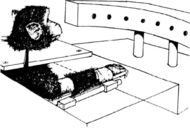
2-1 Monkey is seated on a chair and its arm is fastened to the splint. Targets are located at 5 degrees intervals. In experiments, the monkey was not allowed to see its arm. The room was darkened. [23] . . . . . 18

2-2 Unloaded arm movements of the monkey. In every trial, the initial po-sition was different and monkey managed to reach the target popo-sition.

[23] . . . . 19

2-3 Trajectories of the forearm and EMG data of the biceps observed from

intact monkeys. The bar below the trajectories indicates the duration of the disturbance. A shows the trajectory without disturbances. In B and C, the arm was driven to the target early using external torque. The forearm moved to the position between original and target loca-tions. [24] . . . . 20

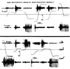
2-4 Trajectories and the EMG data of the forearm movements of the deaf-ferented monkey. Before the target illustration, torque is applied to drive the arm to the target location. When the target is activated, the arm returned back to a position between original and target posi-tion. The upper horizontal bar and the lower horizontal bars indicate duration of servo action and the target light respectively. The continu-ous lines show arm position and the dashed lines demonstrates torque. B=biceps, T=triceps. [24] . . . . 22

2-5 Force fields created by microstimulation . A= Convergence force fields(CFF) around the frog's leg, B= CFF taken from deafferented frog, C= Force fields extracted the region of motoneurons, D= CFF taken by micros-timulation of a spinal cord at 40 Hz for 300 ms, Center= Transverse

section of the spinal cord. [30] . . . . 23

2-6 Snapshots of the equilibrium points following the microstimulation. [25] 23 4-1 One-way coupling for a regular DMP . . . . 30

4-2 One-way coupling for a rhythmic DMP . . . . 30

5-1 Transverse momentum distributions. [8] . . . . 34

5-2 Schematic of the 3DOF helicopter. [8] . . . . 34

5-3 Top view . [81 . . . . 34

5-4 Motor Volt to Thrust Relationship. . . . . 35

5-5 Original maneuver achieved by an operator . . . . 38

5-6 Trajectory generation for the first primitive - pitch . . . . 39

5-7 Trajectory generation for the second primitive - pitch . . . . 40

5-8 Time evolution of primitive-i and primitive-2 merged. . . . . 41

5-9 Tracking performance of the helicopter . . . . 42

5-10 Snapshots of the obstacle avoidance maneuver. . . . . 43

6-1 General structure of the adaptive central pattern generators. [1] . . . . 46

6-2 Time evolution of r with initial conditions 4 and 10 . . . 47

6-3 One-way coupling with a phase difference 7r/4 . . . . 49

6-4 Contraction in region (ii), initial conditions of u1 and u2 are changed from -2,3 to -1,1 respectively . . . . 52

6-5 Contraction in region (iii), initial conditions of u's are changed from -2 to-4 ... ... 53

6-6 variables in region(i) . . . . 53

6-7 Three oscillators . . . . 54

B-i Simulink block diagram of the feedback linearization controller . . . . 63

B-2 Simulink block diagram of a joystick . . . . 64 B-3 Roll controller in the joystick simulink diagram . . . . 65

List of Tables

Chapter 1

Introduction

The role of UAVs (Unmanned Aerial Vehicles) have gained significant importance in the last decades. They have many advantages (agility, low surface area, ability to work in constrained or dangerous places) compared to their conventional precedents. However, a key question still remains: Are we really utilizing their full capacity? In this thesis, we will use a novel approach that combines different fields to give a qualitative answer to this question.

1.1

Thesis outline

We start with showing the background of our approach in Chapter 2.

Chapter 3 contains the analysis of the DMP algorithm using contraction theory. The learning aspect of the algorithm is also studied in this chapter

Chapter 4 describes the method used in coupling the primitives.

Chapter 5 starts with describing the experimental setup and the controller that are used on our application. Next, we describe the Simulations and the Experiments step by step, starting from trajectory learning to the final tests.

Chapter 6 contains the analyzes of Matsuoka's and Hopf oscillator. Chapter 7 contains the extensions of the DMP algorithm.

Chapter 2

Research Approach

2.1

Background

We can classify the background into three fields that each has specific importance.

2.1.1

Biological Motivation

The animal nervous system is an expert in controlling the body to accomplish certain movements despite environmental challenges. For example, a squirrel can climb a tree very quickly despite the many dynamic constraints. We are still far away from explaining how the nervous system controls motion, but there has been a number of studies which lead us closed to the answer.

In the experiments [23], monkeys were used to carry out a movement of a forearm to reach a visual target (See Fig. 2-1) and reward was given if they hold at this position for one second. During this process, their forearm was fastened by an apparatus that lets them extend their forearm in the horizontal plane without the sight of their arm. Tests were performed before and after the medical surgery that deprives the monkeys of a sensory input from their forearm. In both intact and the deafferented monkeys, initial position of the arm changed before the beginning of the movement

(150-200 ms). However, in both cases, the forearm moved to the target precisely.

the initial conditions and the control variable is the equilibrium point achieved by

agonist and antagonist muscles (See Fig. 2-2).

0

Figure 2-1: Monkey is seated on a chair and its arm is fastened to the splint. Targets are located at 5 degrees intervals. In experiments, the monkey was not allowed to see its arm. The room was darkened. [23]

It is also found that the success of the deafferented monkey is closely related to the positions between the body and the arm apparatus. When they changed the posture of the monkey, it was seen that deafferented monkey's approach to the target was inaccurate, although the intact monkey achieved the same movement. This experiment underscores the fact that performance is closely connected with

feedback control.

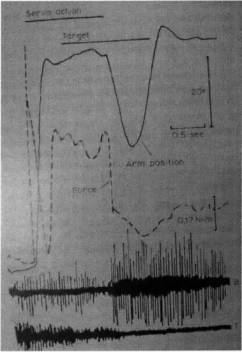
The same experimental setup was used again over monkeys to determine the characteristic of the trajectory [24]. In one experiment, when the intact monkey started to approach the target, a brief torque was applied to drive the elbow quickly to the desired position. However, it was noted that the elbow returned to an intermediate position between starting and the target point before turning back to the target position (See Fig. 2-3). We can see that while returning back to intermediate location, flexor muscles showed EMG (electromyographic) activity.

In another experiment which was performed in deafferented monkeys, the arm was located at the target position and stabilized there using torque motor. The monkey didn't expect a reward, because the target was not illuminated. In addition, the

ARM MOVEMENTS MADE BY PELAFERENTED MONREY

Figure 2-2: Unloaded arm movements of the monkey . In every trial, the initial

position was different and monkey managed to reach the target position. [23]

monkey was insensible to the displacement because of the lack of sensory inputs. In its new position, the target was illuminated. However, instead of staying in the current position, the trained monkey moved its arm first to the location where its arm was originally located and moved it back to the target location (See Fig. 2-4). The last

two experiments suggest that the movement called "virtual trajectory"~ is composed of more than one equilibrium point and CNS (central nervous system) uses this stability of lower level of the motor system to simplify the generation of movement primitives

[241

Experiments on frogs [30, 25] show us another clue to understand the movement primitives. They microstimulated spinal cord and measured the forces at the ankle. This process is repeated with ankle replaced at nine to 16 locations and it is observed that collection of measured forces is always convergent to a single equilibrium point (See Fig. 2-5).

In microstimulation of the spinal cord, the forces acting on the ankle is not sta-tionary. It changes with time. It was also observed that snapshot of these force fields

converge into an equilibrium point (See Fig. 2-6) . These findings also suggest

Figure 2-3: Trajectories of the forearm and EMG data of the biceps observed from intact monkeys. The bar below the trajectories indicates the duration of the distur-bance. A shows the trajectory without disturbances. In B and C, the arm was driven to the target early using external torque. The forearm moved to the position between original and target locations. [24]

trajectory [31].

2.1.2

Imitation Learning

Confucius once said: "By three methods we may learn wisdom: first, by reflection, which is noblest; second, by imitation, which is easiest; and third, by experience, which is the most bitter. Imitation takes place when an agent learns a behavior

by observing the execution of that behavior by a teacher (Bakker-Kuniyoshi [10]).

Imitation is not inherent to humans and is also observed in animals. For example, experiments show that kittens exposed to adult cats manipulate levers to retrieve food much faster than the control group (Galef [27]).

There has been a number of applications of imitation learning in the field of robotics. Studies on locomotion [4, 5, 33], humanoid robots [6, 7],[28], [26], and human-robot interactions [32, 19] have used either imitation learning or movement primitives. The emphasis on these studies is on primitive derivation and movement classification [29]; combinations of the primitives [20, 15, 21, 22, 43, 41] and primitive models [16, 18, 45, 41] in order to extract behaviors.

and combine them consecutively in different initial conditions to generate aggressive maneuvers. Our approach is designed in view of the experiments on frogs and monkeys which suggest that we are faced with an inverse-kinematics algorithm that adapts to the environment and changes in a sequence of equilibrium points irrespective of the initial conditions. The equilibrium points in our algorithm have not necessarily time bounds and we take the original maneuvers from human-piloted flight data.

-J

Figure 2-4: Trajectories and the EMG data of the forearm movements of the deaf-ferented monkey. Before the target illustration, torque is applied to drive the arm to the target location. When the target is activated, the arm returned back to a posi-tion between original and target posiposi-tion. The upper horizontal bar and the lower horizontal bars indicate duration of servo action and the target light respectively. The continuous lines show arm position and the dashed lines demonstrates torque. B=biceps, T=triceps. [24]

A .. 1 C B / 1/' I D \.\ \ .' ~ I I / ~ H / \\ \'~ ~ ~ U / N '~ 54 ~ /

Figure 2-5: Force fields created by microstimulation . A= Convergence force

fields(CFF) around the frog's leg, B= CFF taken from deafferented frog, C= Force fields extracted the region of motoneurons, D= CFF taken by microstimulation of a spinal cord at 40 Hz for 300 ms, Center= Transverse section of the spinal cord. [30]

(di) (b) (c)

cm

Figure 2-6: Snapshots of the equilibrium points following the microstimulation. [25] 1.

Chapter 3

Analysis of DMP

This section outlines the analysis of the DMP algorithm [17] which we later combine using contraction theory.

3.1

DMP Algorithm

DMP is a trajectory generation algorithm which interpolates between the start and end points of a path based on learning. We use the preferred path of the human operator as the learning criterion. The system can be represented by

ri = az(#2(g - y) - z) (3.1)

(3.2)

ry = z

+

where y,

y

#

rV = a(,8z(g - x) - v) _(3.3)

(3.4)

rX v,

where g is the desired end point. Assuming that the f-function is zero, system will converge to g exponentially. The goal of the DMP algorithm is to modify this

exponential path. Therefore, the f-function makes the system non-linear and allows us to generate different trajectories between the origin and the g point.

The f-function is a normalized mixture of Gaussians functions which approximates the final trajectory, i.e. it has the general form

where

ZN Tii f(X, ,g) = -h,

Ti = exp{ -hi (x/g - ci)2}.

(3.5)

(3.6)

3.2

Rhythmic DMPs

The DMP algorithm can also be extended to the rhythmic movements [47] by changing the canonical system with the following:

r = 1 (3.7)

r- = -ap(r - ro) (3.8)

where q corresponds to x in Eq. 3.3 as system, control policy:

a temporal variable. Similar to the discrete

ri = &()3(ym - y) - z)

y = z + f (N QiTi

f(x,

V= exp{hi(cos(O - ci) - 1)}

where ym is a basis point for learning and D = [r cos(), r sin(#)]T.

(3.9) (3.10) (3-11) (3.12)

3.3

Learning of primitives using DMPs

Learning aspect of the algorithm comes into play with the computation of the weights

(wi) of the Gaussians. Weights are derived from Eq.3.1 and Eq.3.2 using the training

trajectory Ydemo and ydemo as variables . Once the parameters of the f-function are learned, then DMP can simply be used to generate the original trajectory. In DMP, spatial and temporal shifts are achieved by adjusting the g and T respectively and

DMP functions as shown below.

" Spatial adjustments: Recall that a function (f) is said to be linear if it has the

property:

f(ax + OX) = af(x) + Of(y) f : RM - R' (3.13)

where x, y . Rm a,

f

Eq.(3.2)] can be seen as a linear system. It is due to the fact that variable v in

f-function is only multiplied by time-varying constant. From linearity, output

(y) is a scaled version of the input (g).

" Temporal adjustments: The second system [(Eq.(3.3) Eq.(3.4)] is linear and

responses against the adjustments of r proportionally . Hence, the multiplier of variable v in

f-function

These arguments can also be extended to the rhythmic DMP for modulations.

3.4

Analysis of DMP Using Contraction Theory

Consider a system

d 6z1 F1 0 Jz1 (3.14)

where zi and z2 represent the first and the second system of DMP respectively. It

can be seen that the second system is contracting without any coupling term and bounded F216zi represents exponentially decaying disturbance. Similar to F₁₁, F2 2 is

contracting in the second equation. Hence, there is a hierarchy among the contracting systems and the whole system globally exponentially converges to a single trajectory. Hierarchical contraction can also be seen in rhythmic DMPs, since the derivatives of

x = r cos() and y = r sin(o) are contracting.

Although the system will eventually contract to the g point, there will be a time delay due to the hierarchy between second and the first system. We can decrease this delay by increasing the number of weights in our equation.

Stability of the DMPs can easily be analyzed. Once the original trajectory is mapped into the DMP, the system behaves linearly for a given input as shown before. Moreover, contraction property guarantees the convergence to a single trajectory. In this perspective, it is easy to show that learning the trajectories is not constrained

Chapter 4

Coupling of DMPs Using

Contraction Theory

In this section, we use partial contraction theory [14] to couple DMPs.

4.1

One-way Coupling

One-way coupling configuration of contraction theory allows a system to converge to its coupled pair smoothly. Theory for the one way coupling states the following:

L1 = f(Xi, t) (4.1)

'2= f(X2, t) + u(Xi) - u(X2) (4.2)

In a given system, if

f

A typical example for one way coupling is an observer design. While the first

system represents the real plant and the second system represents the mathematical model of the first system. The states of the second system will converge to the states of the first system and result in the robust estimation of the real system states. However, for our experiments, we interpret contraction as to imitate the transition between two states. It will be shown in chapter V how the end of one trajectory becomes the initial condition of the second trajectory and contraction accomplishes

S 10 I5 20 25 _0 006 5.5 2 2.5 3 35

Figure 4-1: One-way Figure 4-2: One-way

coupling for a regular coupling for a rhythmic

DMP DMP

the smooth transition.

In DMPs, we couple the two systems using the following equations:

1 = gi - Y1 - 1 + f (yi) (4.3) Q2 = 92 - Y2 - V2 + u(yl) - u(y2) (4.4) u(xi) = gi + f(Xi) (4.5) ZNEiwiv (4.6) f(x, v,g) = * 4 Ti = exp{-hi(x/g - Ci)2 (4.7)

A toy example of the equations listed above can be seen in Fig. 4-1 and Fig. 4-2.

In this setting, Y2 is the first trajectory primitive, which contracts to y, - the second trajectory primitive.

One-way coupling has many advantages over its precedents. In [41], trajectories are achieved by stretching temporal and spatial components of the system and there is a direct relation between initial and end points. Moreover, there are discontinuities in terms of derivatives of the trajectory at the transition regions between primitives. Giese [42] solves the problem of discontinuities by first taking the derivatives of the original trajectories, then combining the derivatives, and finally integrating them

0.6. 300 250 2W 150 100 so

again using initial conditions. However, this method adversely affects the accuracy of the trajectories. Hence, our method improves on [41] and [42] by generating more accurate trajectories independent of initial points. We summarize the advantages for using dynamical systems as control policies as follows:

" It is easy to incorporate perturbations to dynamical systems. " It is easy to represent the primitives.

" Convergence to to the goal position is guaranteed due to the attractor dynamics. " It is easy to modify for different tasks.

" At the transition regions, discontinuities are avoided using initial conditions for

the derivatives.

" Partial contraction theory forces the coupling from any initial condition.

Also in [17], the system is driven between stationary points. However, biological experiments suggest that we are faced with a "virtual trajectory" composed of equi-librium points that has velocity compounds. For this reason, we showed that we can achieve this property by combining nonconstant points.

Chapter 5

Experiments on Helicopter

In this section we apply the motion primitives on the helicopter.

5.1

Experimental Setup and Controller

5.1.1

3 DOF Helicopter

We used Quanser Helicopter (see Figure 5-1) in our experiments. The helicopter is an under-actuated and minimum-phase system having two propellers at the end of the arm. Two DC motor are mounted below the propellers to create the forces which drive propellers. The motors' axes are parallel and their thrust is vertical to the propellers. We have three degrees of freedom (DOF): pitch (vertical movement of the propellers), roll (circular movement around the axis of the propellers) and travel (movement around the vertical base) in contrast with conventional helicopters with six degrees of freedom.

5.1.2

System Dynamics

In system model[8], origin of our coordinate system is at the bearing and slip-ring assembly. The combinations of our actuators form the collective (T,,1 = TL + TR) and

cyclic (Ty, = TL - TR) forces and they are used as inputs in our system. The pitch

Figure 5-1: Transverse momentum distributions. [8]

L

Figure 5-2: Schematic of the 3DOF helicopter.[8]

Left

Right

- 5 L

Figure 5-3: Top view. [8]

travel angle is controlled by the components of thrust. Positive roll results in positive change of angle. The schematics of helicopter are shown in Figures 5-2 and 5-3

Let J_, Jyy, and Jz denote the moment of inertia of our system dynamics. For simplicity, we ignore the products of inertia terms. Then, the equations of motion

are as follows (cf. Ishutkina [8]):

JyyJ

= (TL

+

= -Mglosin(9+ Oo) + (TL + TR)Lcos(#)

= -mgy sin(O) + (TL - TR)lh

" M is the total mass of the helicopter assembly

" rn is the mass of the rotor assembly

" L is the length of the main beam from the slip-ring pivot to the rotor assembly

" 1h is the distance from the rotor pivot to each of the propellers * Drag = { p( L)2 (So + SO sin(#))L

" So and SO are the effective drag coefficients times the reference area and p is

the density of air

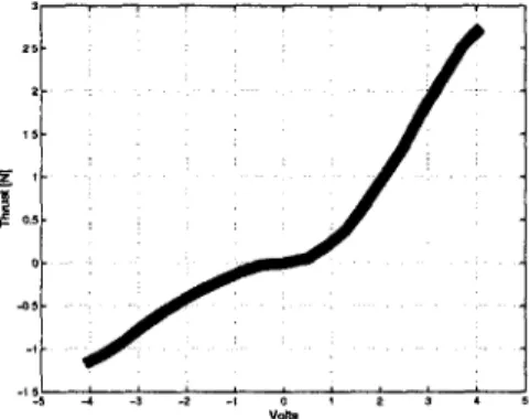
Since the power to the actuators are given by the voltages, a thrust to voltage relationship has been empirically determined and implemented using a lookup table.

Figure5-4[9] 2 0.5 0 -05 -4 -3 -2 -1

Figure 5-4: Motor Volt to Thrust Relationship.

5.1.3

Feedback Linearization

As shown in the above section the system is described by equations which are non-linear in the states, but nonnon-linear in terms of control inputs. In practice, we want to design a tracking controller [11] for a 3DOF helicopter which can track the trajecto-ries in elevation and travel. To use the techniques of input-output linearization [12] and design a tracking controller while avoiding singularities, we reduce the system model to dominant terms:

Si

i i .

.

.

I a a a

Table 5. 1: Parameter Values

Parameter Value Unit Description

M 1.15 kg mass of the rotor assembly

M 3.57 kg mass of the whole setup

MO 0.031 kg effective mass at hover

L 0.66 m length from pivot point to the heli body

la 0.177 m length from pivot point to the rotor

JXX 0.0344 kgm2 moment of inertia about x-axis

Jyy 1.0197 kgm2 moment of inertia about y-axis

Jzz 1.0349 kgm2

moment of inertia about z-axis

JYZ -0.0018 kgM2 _{product of inertia}

JZY -0.0018 kgm2 _{product of inertia}

R 0.1 m radius of the rotor

9 9.8 M/s2 gravitational constant

1 _ 0.004 m length of pendulum for roll axis

l 0.014 m length of pendulum for pitch axis

- -Mgl_{6 o L}

& = sin(9 + -O)+ Lcos(#)Tcol

= Tccmg- _{sin( )} -

L

To achieve tracking tasks we derive the equivalent input:

V = Yd - 2Ai - A2i

with x = [OO)] and z = x - Xd being the tracking error. Since, Eq.5.3 is decoupled from the other two equations and one can use dynamic inversion to write:

Vo - cosin(9 + Oo)

cicos(0)

we can solve for appropriate kd through

tan(#) =VP

(Vo - cosin(9 + 0))c4cos(O)

where c's substitute for the appropriate constants from the dynamic equations. Once the corresponding

#d

Finally, we find TC - V c3sin(#) cyc -C₂ TC01 = VP - c5Teyesin(0)sin(0) c4cos(O)sin()

To use feedback linearization control law, it is necessary to measure all the states of the system. Since only the angles of 3DOF helicopter are measured, we have applied a derivative and a low pass filter to collect the derivatives of the states. Once implemented in Simulink via S-functions, the controller described above is robust and has excellent tracking characteristics.

5.2

Trajectory Generation

In our experimental setup, we used an operator with a joystick to create aggressive trajectories to pass an obstacle. However, generating aggressive trajectories with the joystick is a difficult task even for the operator. Therefore, we designed an augmented control for the joystick to enhance the performance of the helicopter. In particular, we used "up" and "down" movements of the joystick to increase or decrease the T,,, that is applied to the actuators. For the "right" and "left" movements of the joystick,

we preferred to control the roll angle using PD control.

In the original maneuver, the obstacle's distance and the highest point are in the coordinates where L and 0 angles are 220 and 60 respectively and the helicopter starts with coordinates where ) = 28, 0 = 317 and

#

350 Elevation 300_ Pitch Travel 250- 200- 150-100

/

Figure 5-5: Original maneuver achieved by an operator

5.3

Trajectory Learning

To fly over different obstacles, the acquired primitive is segmented into two primitives at the highest pitch angle. Figures 5-6 and Fig. 5-7 show the results of DMP algorithm for the pitch angle. Since the Quanser Helicopter has 3-DOF, for any given trajectory, we use DMP to approximate paths on roll and travel components as well. In Fig.

5-6, the top left graph is a result for the pitch angle, where green line represents the

operator input for the trajectory and the blue line represents the fitting that the DMP computes. Other figures show the time evolution of the DMP parameters. It can also be seen that the generated trajectories capture the operator's driving characteristics.

y & y

demo,

60

40.

20

0

-201

0

5

10

time (sec)

parameter x

50,

40

30

20

0

5

10

time (sec)

30

20

10

0

yd & yd demo

time

(sec)

parameter v

150,

100-501

0

0

5

10

0

1

ydd & ydd demo

-50L

0

6

10

time (sec)

parameter z

000

500

0

-500

0

5

10

time (sec)

Figure 5-6: Trajectory generation for the first primitive - pitch

5.4

Synchronization of primitives

The two primitives created in the previous sections are defined as trajectories between certain start and end points. However, the end point of the first trajectory does not necessarily matches with the starting point of the second trajectory. We use the contraction theory to force the first trajectory to converge to the second trajectory.

60

-20,

-40

50

40,

30

0

5

parameter x

20'

0

5

time (sec)

10

0'

-20

-30

0

0

0

yd & yd demo

time (sec)

parameter v

5

20

0

-20

100

0

-100

-200

0

ydd & ydd demo

5

parameter

z

5

C

time' (sec),

Figure 5-7: Trajectory generation for the second primitive -pitch

However, since we want to use the contraction as a transition between two trajectories, coupling is enabled towards the end of first primitive. Figure 5-8 shows how the two trajectories evolve in time. In the first primitive, the goal positions of L and 0 angles are changed to 1500 and 500 respectively, where original angles are 0 = 2200 and

0 = 600. In the second primitive, the goal position of the 0 angle is changed from

317' to 3000. Solid line shows the travel, dashed line shows roll, and dash-dot line

shows the pitch angles while the vertical dotted line indicates the switching time from the first primitive to the second one. It can be seen that the trajectories fit each other smoothly at the transition points.

Final Trajectory

200 400 600 8M ) 1000

tlme(sec) x 100

1210 1400 1600 1800

Figure 5-8: Time evolution of primitive-1 and primitive-2 merged.

5.5

Experiments on the Helicopter

Tracking performance of our helicopter with respect to the desired trajectory is shown in Figure 5-9. It can be seen that the helicopter followed the desired (0 and 9) angles almost perfectly. The trajectory of the roll angle is different than the desired since we control two parameters (V) and 9) and the goal positions of the DMPs are different. However, it can be seen that they follow the same pattern. The last part of the roll trajectory manifests an oscillation which can be prevented by roll control, since the other parameters are almost constant. The tracking performance can further be improved by applying discrete nonlinear observers to get better velocity and acceleration values. Figure 5-10 shows snapshots of the maneuver.

300 250 200 150 100 - travel - - roll --- pitch - - .- ... ..-.- ...-.- . -.-. -.-. -.- .- . connection of primitives - - -- -- ----- ---. ... .-. .............-. .. ..- -...-. ..-. ... ...-.- ..- . -5, 50 0 -100 A ... ... ... .. ... ... .. ... . ... ... .. .... ... . ... ... ... .. .. .... . . .I ... ... ... ... ... ... .. . . .. . . . ... ... ... ... ... ... ... .

GA Actual pitch Actual roll - - -.. - -. S Actual travel--- .. --. Reference pitch -Reference roll -... Reference travel 2

(a) 1 (b)2

(d) 4 (e) 5 (f) 6

(g) 7 (h) 8 (i) 9

Figure 5-10: Snapshots of the obstacle avoidance maneuver.

Chapter 6

Analysis of Oscillators Using

Contraction Theory

In biological systems, various types of oscillations and rhythmic movements can be observed. Studies on these behaviors suggest that spinal cord possesses central pattern generators (CPGs) to have such a property [49]. In this perspective, there are several types of CPG models in the literature. The purpose of this chapter is to analyze two

of them (the Hopf oscillator and Matsuoka's oscillator) using contraction theory.

6.1

Hopf Oscillator

In [46], Ijspeert design a generic central pattern generator (CPG) that can adapt to given periodic signals. In the model, he represents the periodic function as a combination of Hopf oscillators like fourier series and each oscillator's frequency and amplitude are learned using Hebbian learning (See Fig.6-1). Here, we will analyze the Hopf oscillators after learning. The system can be represented by

y=7(p - r 2 )x - Wy (6.1)

where r Vx2 + y2

and w is the coupling term which is defined through learning.

LTO2

Figure 6-1: General structure of the adaptive central pattern generators.[1]

First, we assume that we have a system without coupling:

S= 7(- r2

)x

p

(6.3)

(6.4)

In polar coordinates, the system becomes

r = Y(p - r2)r (6.5)

From Lyapunov, it is easy to show that r converges to ,/7 and the jacobian of system:

Of

ar

2 _(6.6)

Since r2 -+ P, the system is contracting as shown in Fig. 1.

The jacobian in cartesian coordinates is also contracting. The equations of oscil-lator are as follows

0 0:1 0.2 0.3 0.4 0.5 0.6 0.7 .S 0.9 1

Figure 6-2: Time evolution of r with initial conditions 4 and 10

=

'-y(pL

)

Ox

=

7(p

92)

ay

Since 2 + y2 -+ /u, our equations contract and eventually become

af -= -2yx2 Of Oy (6.7) (6.8)

Theorem 1 if we couple Eq. 6.3 and Eq. 6.4 as it is done in Hopf oscillators, then x

and y will converge to each other exponentially with a phase difference 7r/2 regardless of initial conditions.

x(0) and y(O), we define

Of . f

g(x, y, t)= - -- wy= --- wx (6.9)

Ox Oy

and construct the auxiliary system Of

= _{-- +g(x, y, t) (6.10)}

This system is contracting since the function 2 is contracting and all solutions of z_az

converges into a single trajectory. Since z = x and z = y = xj are two particular

solutions, this implies that x and y synchronize with phase difference 7r/2.

Even after coupling, we still preserve the Eq. (6.6) in polar coordinates and the system contracts. Hence, we can apply partial contraction theory for different tasks. In particular, we will use one-way synchronization and rotational transformation (see

Keehong [52]) to lock the oscillators with phase differences as it is done in [51]. The

equations can be represented by

:4 =

y(

y1

2= 7(t - r2)x2 - O(x 2 - cos(9)xi + sin(9)yl) (6.13)

V2 =7(P - r2)y2 - O(Y2 - sin(6)x1 - cos(9)yi) (6.14)

where ri = x +y?, i = 1, 2 and 6 is the phase difference desired between oscillators.

The example of phase-locking can be seen in Fig.6-3.

6.2

Matsuoka's Oscillators

In [44], Matsuoka design mutual inhibition networks represented by a continuous-variable neuron model to generate oscillations (see details for [44]). The system can be represented by

0 5 10 15 20

frme(sec)

25

Figure 6-3: One-way coupling with a phase difference 7r/4

il = -U1 - Wy₂ - 3v1

+ uO

yj = f(uj) f(uj) = max(0, uj) (i = 1, 2)

U0 > 0

where ui is the inner state of the neuron; yj is the output of the neuron; vi is the self inhibition variable; uo is the external output; w is the coupling constant; r is the time constant. Since the system contains non-smooth functions (yi) in it, we will

investigate the Matsuoka's oscillators in four regions as it is done in [50].

(i) For ui > 0 and u2 > 0, we can derive the equations below:

-I 4 xy 2X

. iA

~~

~~~

T ₁ = -ij1 - (-r,61 + vj) - w(TZi2 + v2) - OV1 + uO

r62 = - 2 - (T712 + v2) - w(T;1 + VI) - ,v2 + uo

From Eq. (6.19) and Eq. (6.20), we have

r(i + )= -(T + I + TW)(i + '₂) - (0+ 1 + w)(vi + v2)+

2uo

and also

lil

(6.19)

(6.20)

(6.21)

(6.22)

From the equations above, it is easy to say that variables ui + u2 and v1 + v2 will

converge to equilibrium points, if the constants that multiplies the variables are pos-itive. However, there are two solutions in terms of u's and v's. For u's, first solution

is ui = 0, u2 = 0 and the second one, which is of our interest, is Ui = -u 2. To have

the second solution, our system should be unstable. Therefore, eigenvalue analysis is done to have proper variables. From analyzes, it is found that one of the conditions listed below should be accomplished.

f

3

(ii) For ui > 0 and U2 < 0, we can derive the equations below:

r?1 = -(r + 1) 1 - (0 + 1)vi + uo TV2 = -V2

for ''s become

+uo

r1i= - - UO+U0

/+1

rzi2 = -U2 - WU1 + UO

Therefore, u1 - u and u2 -- I3w

-(iii) For ui > 0 and u2 < 0 , solution is a symmetric version of the region (ii).

(iv) For ui < 0 and u2 < 0, we can derive the equations below:

7i1 = -Ui - 3V1+ Uo (6.23) (6.24) 2 = -U 2 - Ov2 + Uo T1i = -Vi r7 ₂ = -V2 (6.25) (6.26)

From ODE analysis, it can be concluded that v1, v2 - 0 and U1, u2 -- uo.

Theorem 2 System has periodic oscillations if and only if # > w - 1 and w > 1 + 1/r

Proof: Region(ii), region(iii) and region(iv) contract (see Fig. 6-4 and Fig.6-5) and converge to a virtual equilibrium point in region(i), if we have the following conditions: / > -1 and w > 1 + 1/r. In oscillations, there should be a continuous chain reaction among regions. To achieve such a property, parameters of the region(i) should have at least one of these conditions: < w - ,3< -w - 1, w <-1 - or w > I +

Therefore, overall conditions for parameters are 3 > w - l and w > I + l/T. Since the system converges to a specific trajectory in the contracting regions , dynamic system in region(i) itself also generates a specific trajectory because of the same initial conditions. Moreover, in region (i) variables are forced to change signs . They have symmetry and receive the phase difference among each other as well.

0 5 10 15 20 25

Figure 6-4: Contraction in region (ii), initial conditions of ui and u2

-2,3 to -1,1 respectively

are changed from

Remark:

As compared to two neurons, intuitively, we can derive the similar conditions for three-neuron ring in [44]. In this case, anti-synchronization in region (i) ,where

u1, u2, U3 > 0, can be achieved (see Fig.6-6) given proper parameters. If we force the

other regions to converge to the region(i) with adjusted parameters then the desired variables can synchronize with a phase difference as shown in Fig.6-7.

U2

V1

...V2

...

-A U1 .vl v2 0 --2 -3 --0 2 4 6 8 10 12 14 16 18 20

Figure 6-5: Contraction in region (iii), initial conditions of u's are changed from -2 to -4

-4

-1

0 5 10 15

Figure 6-6: variables in region(i)

-uI -- u2 0 - u3 -v1 . v2 0 .3 10 0 0

6

0.5 0 -0.5 -- U1 U2

-12-

Chapter

7

Extensions of DMP

7.1

Dynamical System with First-Order Filters

DMP algorithm can be improved by replacing the first system with the equations shown below: r9 + aly = a1x 1 + a2x = a2g +

-f

7r

f

By introducing two first-order filters, we can guarantee the stability of the system

against time varying parameters like r(t) or g(t) . Since the system is linear without f-function (Eq.3.11), we can achieve learning and modulation properties of DMP using the

f

7.2

Two-way Synchronization of DMPs

Experiments on frog's spinal cord [30, 25, 48] suggest that movement primitives can be generated from linear combinations of vectorial force fields which lead the limb of a frog to the virtual equilibrium points. In [48], it is also pointed out that vectorial summation of two force fields with different equilibrium points generate a new force field whose equilibrium point is at intermediate location of the original equilibrium points. In this perspective, we will synchronize DMPs to generate a new primitive whose trajectory is a linear combination of synchronized trajectories. Consider a system

#i = f(yi, t) + K(u(y2) - u(yi)) (7.4)

Y2 = f(y₂, t) + K(u(yi) - u(y₂)) K > 0 (7.5)

Where yi and Y2 represent the first and the second primitive respectively. From par-tial contraction theory, we can say that y, and Y2 converge together exponenpar-tially, if

f

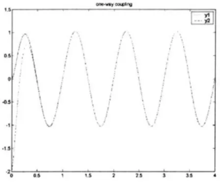
synchro-nization using contracting inputs. In Fig.7-1, new primitive is a linear combination of sine and cosine primitives.

I \' \

-7 1sine \c-sneo zation

0.5-0

--1.5

0 5 10 0ii 2\' 3 350 4

Skne

Chapter 8

Conclusion

In this thesis, we use a novel approach, inspired by biological experiments, which uses control primitives to imitate the data taken from human-performed obstacle avoidance maneuver. In our model, DMP computes the trajectory dynamics so that we can generate complex primitive trajectories for given different start and end points, while one-way coupling ensures smooth transition between primitives at the (possible unstable) equilibrium point. We demonstrate our algorithm with an experiment. We generate a complex, aggressive maneuver, which our helicopter could follow within a given error bound with a desired speed. We will conduct future research on different combinations of primitives using partial contraction theory.

Appendix A

Contraction Theory

The basic theorem of contraction analysis [13] can be stated as

Theorem 1 (Contraction) Consider the deterministic system

=

f(x, t)

(A.1)

where f is a smooth nonlinear function. If there exist a uniformly invertible matrix associated generalized Jacobian matrix

af

F

(E +

e-)e-1

1x (A.2)

is uniformly negative definite, then all system trajectories converge exponentially to a single trajectory, with convergence rate IAmax|, where AmaxiS the largest eigenvalue

of the symmetric part of F. The system is said to be contracting.

It can be shown conversely that the existence of a uniformly positive definite metric

M(x, t) =

e(x,

with respect to which the system is contracting is also a necessary condition for global exponential convergence of trajectories. Furthermore, all transformations

E

corresponding to the same Mlead to the same eigenvalues for the symmetric part F, of F, and thus to the same contraction rate

|AmaxI-In the linear time-invariant case, a system is globally contracting if and only if it is strictly stable, with F simply being a normal Jordan form of the system and Othe coordinate transformation to that form.

Contraction analysis can also be derived for discrete-time systems and for classes of hybrid systems.

A simple yet powerful extension to contraction theory is the concept of partial

contraction, which was introduced in [14].

Theorem 2 (Partial contraction) Consider a nonlinear system of the form

k = f(x, x, t)

and assume that the auxiliary system

= f(y, x, t)

zs contracting with respect to y. If a particular solution of the auxiliary y-system verifies a specific smooth property, then all trajectories of the original x-system verify this property exponentially. The original system is said to be partially contracting.

Indeed, the virtual, observer-like y-system has two particular solutions, namely

y(t) = x(t) for all t > 0 and the solution with the specific property. Since all

trajectories of the y-system converge exponentially to a single trajectory, this implies that x(t) verifies the specific property exponentially.

Appendix B

Simulink Diagram

Figures show the Simulink block diagrams used in our hardware.

X, des Tcol X, states Tcyc Controller Tool Coll: T1+T2 \mt Left (1) Sat I Diff: T1-T2 *vft Right (2) Sat 2 Convert to volts T rye Hell 3D

Figure B-1: Simulink block diagram of the feedback linearization controller

0 'Time * Xdesired _" Controller Subsystem Constani Time-Base Bad Link

- TrM l e

Heli 3D

Coll stick b o 5fl -i c k

Sroll

Cyc stick bCye stick Ot?

Joystick Inputs CtrI

Cyjc joystick

Cyc stic

Bad Link-2

AnalogInputDead Zone2sat2: p/m a.Coll joystick

C oll stick

LBad Link

Analog Input 0.3 Dead Zone3satil: p/m 3.6 Gain

roll

S0.04

s+10 Col I joysti I c

Appendix C

Codes of Trajectory Generator S

function

* traj-generator.C

* The calling syntax is:

* INPUTS:

* OUTPUT

* COMMENTS:

% I want to thank Selcuk Bayraktar and Mariya A. Ishutkina for their contributions. This code is modified over their previous work.

#define SFUNCTIONLEVEL 2 #define SFUNCTIONNAME traj-generator

#include "simstruc.h" #include <stdlib.h> #include <stdio.h> #include <math.h>

/* #define Time 0 #define GlobalOn 0 //#define ARRAYSIZE 1797 / *=== = == = = == ==* * S-function methods * /* Function: mdlInitializeSizes * Abstract:

* The sizes information is used by Simulink to determine the S-function * block's characteristics (number of inputs, outputs, states, etc.).

static void mdlInitializeSizes(SimStruct *S) {

ssSetNumSFcnParams(S, 0); /* Number of expected parameters */ if (ssGetNumSFcnParams(S)

!=

/* Return if number of expected != number of actual parameters */ return; } ssSetNumContStates(S, 0); ssSetNumDiscStates(S, 0); if (!ssSetNumInputPorts(S, 2)) return; ssSetInputPortWidth(S, 0, 1); ssSetInputPortWidth(S, 1, 1);

ssSetInputPortDirectFeedThrough(S, 0, 1); ssSetInputPortDirectFeedThrough(S, 1, 1); if (!ssSetNumOutputPorts(S, 1)) return; ssSetOutputPortWidth(S, 0, 10); ssSetNumSampleTimes(S, 1); ssSetNumRWork(S, 0); ssSetNumIWork(S, 0); ssSetNumPWork(S, 0); ssSetNumModes(S, 0); ssSetNumNonsampledZCs(S, 0); ssSetOptions(S, SSOPTIONEXCEPTIONFREECODE);

}

* This function is used to specify the sample time(s) for your

* S-function. You must register the same number of sample times as * specified in ssSetNumSampleTimes.

static void mdlInitializeSampleTimes(SimStruct *S) { ssSetSampleTime(S, 0, INHERITEDSAMPLETIME); ssSetOffsetTime(S,0,FIXEDINMINORSTEPOFFSET); } /* static void mdlInitializeSampleTimes(SimStruct *S) {

the simulation */ /* ssSetOffsetTime(S, 0, 0.0); /* use

descrete sample

/* }

#undef MDLINITIALIZECONDITIONS /* Change to #undef/define to

remove function */ #if defined(MDLINITIALIZECONDITIONS) /* Function: mdlInitializeConditions

* Abstract:

* In this function, you should initialize the continuous and discrete

* states for your S-function block. The initial states are placed * in the state vector, ssGetContStates(S) or ssGetRealDiscStates(S).

* You can also perform any other initialization activities that your

* S-function may require. Note, this routine will be called at the

* start of simulation and if it is present in an enabled subsystem

* configured to reset states, it will be call when the enabled subsystem

* restarts execution to reset the states.

static void mdlInitializeConditions(SimStruct *S)

{ }

MDLINITIALIZECONDITIONS */

#define MDLSTART /* Change to #undef to remove function */ #if defined(MDLSTART) /* Function: mdlStart

* Abstract:

* have states that should be initialized once, this is the place * to do it.

static void mdlStart(SimStruct *S) {

// controller-engaged = 0;

}

/* Function: mdlOutputs

* Abstract:

* In this function, you compute the outputs of your S-function

* block. Generally outputs are placed in the output vector, ssGetY(S).

static void mdlOutputs(SimStruct *S, intT tid)

{

/* inputs */

InputRealPtrsType uOPtrs = ssGetInputPortRealSignalPtrs(S,0); InputRealPtrsType ulPtrs = ssGetInputPortRealSignalPtrs(S,1);

/* Time */ /* Controller*/

static realT pitch-inputl[1700] ={25.4039, 25.4039, 25.4039,

static realT pitch-input2[1700] ={0.0000, 0.0000, -0.0000, ..

static realT pitch-input3[1700] ={0.0000, -0.0000, ... };

static realT rollinputl[1700] ={0.4395, 0.4395, 0.4395, ... };

static realT rollinput2[1700] ={0.0000, 0.0000, 0.0030, ... ;

static realT travelinputl[1700] ={-82.9989, -82.9989,...};

static realT travelinput2[1700] ={0.0000, 0.0000,...};

static realT travelinput3[1700] ={0.0000, -0.0003, ...};

realT Timecurrent = *uOPtrs[0];

int_T times=0;

/*realT pitch pitch-inputl[times]; realT pitch_d

pitch-input2[times]; realT pitch-dd pitch.input3[times]; realT travel travel-inputl[times]; real-T travel-d travel-input2[times]; realT traveldd travel-input3[times]; realT roll

roll-inputl[times]; real-T roll-d roll-input2[times]; realT roll-dd roll-input3[times]; */

realT GlobalOn = *ulPtrs[0]; static realT Timel =0;

/* outputs */

realT *yO = ssGetoutputPortRealSignal(S,0); /* xdesired states */

/* code starts here */

if ((GlobalOn >= 1.0)) {// if GlobalOn