Controllable vapor microbubbles for use in bioparticle actuation

MASSACHUSETTS INSTITUTE OF TECHNOLOGY JU L 0 8 2003 LIBRAR IES BARKER B.S. Cornell University (1996)

D.I.C. Imperial College London (1997) S.M. Massachusetts Institute of Technology (1999) Submitted to the Department of Mechanical Engineering in partial fulfillment of the requirements for the degree of DOCTOR OF PHILOSOPHY IN MECHANICAL ENGINEERING

at the

MASSACHUSETTS INSTITUTE OF TECHNOLOGY June 2003

@ Massachus S5 tute offchnology 2003. All rights reserved.

Author ... . .. ...

Deppartment of Mechanical Engineering April 28, 2003 Certified by ...

V--I----Martin A. Schmidt Professor of Electrical Engineering Thesis Supervisor

C ertified by ... ...

Mehmet Toner

Professor of Biomnedion Fnaineering. Mass. Gen. HosoitAl qnrl Harvard Medical School

Thesis Supervisor

Certified by ...

Martha Gray Edward Hood Taplan Professor of Electrical Engineering Thesis Supervisor C ertified b y ... Bora Mikic

-4 " Pr essor of Nechanical Engineering

Ch~airm n of Thesis Committee Accepted by ...

..

...

Ain Sonin Chairman, Committee on GradTIVIdents

CONTROLLABLE VAPOR MICROBUBBLES FOR USE

IN BIOPARTICLE A CTUA TION

by

CONTROLLABLE VAPOR MICROBUBBLES FOR USE IN

BIOPARTICLE ACTUATION

by

Rebecca Braff Maxwell

Submitted to the Department of Mechanical Engineering on April 28, 2003, in partial fulfillment of the

requirements for the degree of

Doctor of Philosophy in Mechanical Engineering

ABSTRACT

In this thesis, we present guidelines for using thermally formed microbubbles as a means of fluidic actuation. The use of microbubbles is attractive due to the simple fabrication and operation of such devices, however, prior work in this area was hindered

by several issues inherent to vapor bubble formation that severely limited the reliability

of bubble-based devices. It has been shown in this thesis that it is possible to control the location at which bubbles form and the size of the bubbles, as well as to achieve

repeatable and reduced bubble formation temperature, and to create bubbles that collapse completely in less than 10 seconds.

The achievement of controllable microbubbles makes possible many microfluidic applications, one of which we will demonstrate in this work. We have built a device that is capable of capturing, holding, and selectively releasing single bioparticles using microbubble actuation. This bioparticle actuator could be scaled into an array for the analysis of a large population of individual cells.

Thesis Supervisor: Martin A. Schmidt Title: Professor of Electrical Engineering Thesis Supervisor: Mehmet Toner

Title: Professor of Biomedical Engineering, Massachusetts General Hospital and Harvard Medical School

Thesis Supervisor: Martha Gray

Title: Edward Hood Taplan Professor of Electrical Engineering Chairman of Committee: Bora Mikic

ACKNOWLEDGEMENTS

This work was sponsored in part by the National Science Foundation, and the Alliance for Cellular Signaling. I would like to thank my advisors, Marty Schmidt, Martha Gray, and Mehmet Toner for all of their support and guidance throughout this thesis. Working on this project has been a wonderful experience, and I thank them for giving me this exciting opportunity. Each of them brought different perspectives and areas of expertise to the group and it was truly a privilege to work with them. I'd also like to thank Bora Mikic for being the chair of the committee and giving me so much advice throughout the project. He always made time to meet with me when I needed help, and was a pleasure to work with.

Thanks to everyone in the Schmidt group- present and past. I'd particularly like to thank Xue'en Yang for all of her advice and assistance with my thermal modeling and MATLAB, and Antimony Gerhardt for doing some of the testing when she was a UROP student and carrying on with the work now that she is a grad student. Christine Tsau and Ole Neilson also helped with all kinds of things in the lab, and out. I would not have been able to get my Labview test setup working so quickly without all the help I received from Lodewyk Steyn, and I'm very grateful for all of his electronic expertise. I'd also like to thank Samara Firebaugh and Joel Voldman for their guidance while they were still students, when I was beginning this project. I'm also grateful to Anne Wasserman and Pat Varley for all of their administrative assistance during my time at MIT- they certainly helped make life a lot easier. I'd also like to thank Debb Hodges-Pabon for having such a great personality and adding so much life to the MTL.

Thanks also goes to the staff of the Microsystems Technology Laboratory. I received so much help in the lab from Dennis Ward, Kurt Broderick, Joe Walsh, Bob Bicchieri, Bernard Alamariu, Dan Adams, Vicky Diadiuk, and Gwen Donahue. I'd also like to thank Arturo Ayon and Tom Takacs for their help with STS etching. I would like to thank the people at Surface Technology Systems who did the quartz etching on my final test samples.

I'd especially like to thank my friends and family for all of their love and support

outside of the lab. Afternoon tea with Laura, and evenings of eating chocolates and hanging out with Amy helped me make it through without losing my mind entirely. My parents and brother have given me love and encouragement from the beginning, and I

want to thank them for everything that they have done for me.

I must also acknowledge my puppy, Schafer, who made great contributions to the

writing of this thesis. She is certainly a canine genius.

Lastly, I would like to thank Brian for being wonderful and believing in me through it all, even when I was nearly impossible to live with. I couldn't have done this without you.

TABLE OF CONTENTS

1. IN TR O D U CTIO N ... 13

1.1 BACKGROUND AND SIGNIHCANCE... 13

1.1.1 The Microfabrication-Based Dynamic Array Cytometer... 14

1.1.2 M icrofluidic Actuation ... 15

1.1.3 Cell M anipulation M EM S D evices... 18

1.2 O BJECTIVES... 21

1.3 OVERVIEW OF DEVICE FOR MICROBUBBLE ACTUATION ... 21

1.4 THESIS ORGANIZATION ... 22 2 TH EO R Y A ND M O D ELING ... 24 2.1 BUBBLE N UCLEATION ... 24 2.1.1 H om ogeneous N ucleation ... 24 2.1.2 H eterogeneous Nucleation... 26 2.2 THERM AL M ODELING... 27

2.2.1 Finite Elem ent M odel ... 28

2.2.2 Analytical M odel... 30

2.2.3 Finite D ifference M odels... 34

2.3 BUBBLE COLLAPSE ... 41

2.3.1 Phase Change Collapse... 41

2.3.2 D iffusion Collapse... 43 3 D ESIG N ... 46 3.1 RESISTIVE H EATERS... 46 3.2 BIOPARTICLE A CTUATOR ... 50 3.3 FLOW SYSTEM ... 52 4 FA BR ICA TIO N ... 54 4.1 QUARTZ PROCESS ... 54 4.2 SILICON PROCESS... 57 4.3 D EVICE A SSEMBLY ... 58 5 EXPERIMENTAL METHODS... 60

5.1 SAMPLE PREPARATION FOR RESISTOR TESTING... 60

5.1.1 Calibration ... 60

5.1.2 W ater Preparation... 62

5.2 FI ST G ENERATION TESTING ... 62

5.3 SECOND GENERATION TESTING M ETHOD ... 65

5.3.1 Test Apparatus... 65

5.3.2 Repeatability of Resistor H eating ... 67

5.3.3 Bubble Form ation Temperature... 67

5.3.4 Energy D ependence of Bubble Size... 69

5.3.5 Bubble Dynamics... 70

5.3.6 Cycling ... nam.... ... ... 7]

6.1 GENERAL EFFECT OF CAVITIES ON BUBBLE FORMATION (USING THE FIRST

GENERATION TESTING M ETHOD)... 72

6.2 SECOND GENERATION RESISTOR TESTING ... 75

6.2.1 Repeatability of Resistor Heating ... 75

6.2.2 Bubble Formation Location ... 76

6.2.3 Bubble Formation Temperature... 77

6.2.4 Bubble Collapse Time ... 79

6.2.5 Energy Dependence of Bubble Size... 80

6.2.6 Bubble Dynamics... 82

6.2.7 Cycling ... 90

6.3 COMPARISON OF FIRST GENERATION AND SECOND GENERATION RESULTS... 93

6.4 COMPLETE DEVICE... 96

7 DISCUSSION AND CONCLUSIONS ... 98

7.1 OVERVIEW ... 98

7.2 DISCUSSION OF FIRST GENERATION RESULTS ... 98

7.3 DISCUSSION OF SECOND GENERATION RESULTS ... 99

7.3.1 Bubble Formation Location ... 99

7.3.2 Bubble Formation Temperature...102

7.3.3 Bubble Dynamics... 104

7.3.4 Dependence of Bubble D iameter on Energy ... 105

7.3.5 Bubble Collapse ... 106

7.3.6 Cycling ... 107

7.4 FUTURE W ORK... 108

7.4.1 Controllable Bubble Formation...108

7.4.2 M icrobubble Bioparticle Actuator ... 109

7.5 CONCLUDING REMARKS... 110

8 APPENDIX ... 111

8.1 APPENDIX A: QUARTZ PROCESS ... 111

8.2 APPENDIX B: SILICON PROCESS ... 113

8.3 APPENDIX C: DEVICE ASSEMBLY PROCESS... 116

8.4 APPENDIX D: MATLAB CODE FOR FINITE DIFFERENCE MODEL- LINE HEATER 117 8.5 APPENDIX E: MATLAB CODE FOR FINITE DIFFERENCE MODEL- FOLDED HEATER ... 121

FIGURES

Figure 1-1 pDAC system diagram (courtesy of Joel Voldman) ... 15

Figure 1-2 Illustration of the Hitachi cell capture plate ... 20

Figure 1-3 Schematic of the operation of the device is shown. ... 22

Figure 2-1 Thermodynamic pressure-volume diagram[60]. ... 25

Figure 2-2 Schematic of finite element model ... 28

Figure 2-3 Results of finite element simulation of resistive line heater...29

Figure 2-4 Schematic and boundary conditions for thermal model of resistor... 30

Figure 2-5 Thermal circuit model of heater, water, and quartz system. ... 31

Figure 2-6 Plot of average heater temperature as a function of time. ... 34

Figure 2-7 Comparison of steady state temperature of heater . ... 34

Figure 2-8 Two resistor geometries modeled... 35

Figure 2-9 Sample control volume for finite difference model. ... 36

Figure 2-10 Meshed finite difference model of line heater... 37

Figure 2-11 Finite difference model temperature distribution results...38

Figure 2-12 Schematic and boundary conditions for folded resistor model...39

Figure 2-13 Results of finite difference simulation for the folded resistor...40

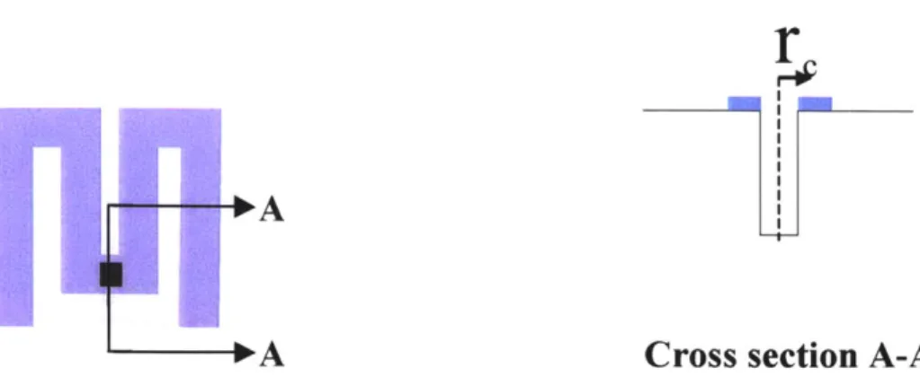
Figure 3-1 Resistive heater with cavity etched into substrate. rc is the cavity radius. ... 47

Figure 3-2 Illustration of the effect of hydrophobic surface treatments. . ... 47

Figure 3-3 Illustration of surface treatments for the resistive heaters. ... 48

Figure 3-4 Resistive heater geometries. ... 48

Figure 3-5 On the left is a folded resistor... 49

Figure 3-6 Schematic of components and dimensions of the microbubble cell actuator.. 50

Figure 3-7 Operation of the microbubble cell actuator...51

Figure 3-8 Schem atic of flow cham ber ... 52

Figure 3-9 Dim ensions of flow chamber... 53

Figure 4-1 Fabrication process for quartz heater layer. ... 55

Figure 4-2 SEMs of 10gm wide trenches on quartz wafers etched by STS. . ... 56

Figure 4-3 Micrograph of completed resistive heater with cavity. ... 56

Figure 4-4 Silicon bioparticle manipulation layer fabrication process. ... 57

Figure 4-5 SEM of capture well and bubble jet channel on silicon layer...58

Figure 5-1 Apparatus used to calibrate resistors ... 60

Figure 5-2 Plot of temperature versus normalized resistance used to calibrate resistors.. 62

Figure 5-3 A typical I-V curve generating in the testing of a line heater ... 63

Figure 5-4 The heater temperature curve generated using the I-V curve...64

Figure 5-5 Schematic of test apparatus for second generation testing...66

Figure 5-6 The three resistor configurations tested. ... 67

Figure 5-7 Heating curve for a folded resistor tested using the LABVIEW program...69

Figure 6-1 A CYTOP-coated platinum line heater with a cavity. ... 72

Figure 6-2 Resistor temperatures at bubble formation ... 73

Figure 6-3 Repeatability of resistor temperature at bubble formation. ... 74

Figure 6-4 Bubble collapse time as a function of maximum bubble size . ... 75

Figure 6-5 Plot of average heater temperature versus time for a 4 volt, 50ms pulse...76

Figure 6-6 Folded heater with etched cavity... 77

Figure 6-9 Plot of bubble collapse time versus initial bubble diameter ... 80

Figure 6-10 Plot of bubble diameter versus total energy applied to the heater...81

Figure 6-11 Plot of heater temperature versus time for a 40ms voltage pulse...82

Figure 6-12 Plot of heater temperature versus time for an 80ms voltage pulse...83

Figure 6-13 Above is a plot of heater temperature versus time ... 84

Figure 6-14 Above is a plot of heater temperature versus time ... 85

Figure 6-15 Above is a plot of heater temperature versus time . ... 86

Figure 6-16 Above is a plot of heater temperature versus time ... 87

Figure 6-17 Above is a plot of heater temperature versus time. ... 88

Figure 6-18 Captured video frames from the t=2000ms voltage pulse... 90

Figure 6-19 Plots of the heater temperature versus time ... 91

Figure 6-20 Plots of the heater temperature versus time ... 92

Figure 6-21 The plot on the left compares the apparent bubble formation...94

Figure 6-22 The plot on the left compares the apparent bubble formation... 94

Figure 6-23 The plot on the left compares the apparent bubble formation ... 95

Figure 6-24 Plot of apparent bubble formation temperature corrected ... 96

Figure 6-25 Sequential photos of device operation during bead capture...97

TABLES

Table 2-1 Thermodynamic superheat limit of water... 26

Table 2-2 Heater temperature distribution results from finite difference model. ... 40

Table 3-1 Resistor geom etries used in testing... 50

Table 5-1 Resistor characteristics for bubble formation temperature testing. ... 68

Table 5-2 Testing parameters for bubble diameter/collapse time testing ... 70

Table 5-3 Test parameters for bubble dynamics testing. ... 71

Table 6-1 Average apparent bubble formation temperature . ... 77

Table 6-2 Results of bubble size/energy testing... 81

Table 6-3 Apparent bubble formation temperature data . ... 93

1. INTRODUCTION

Microfluidics is becoming increasingly important to the success of a wide variety of micromachined devices, particularly those with biological applications. With the reduced dimensions that are now easy to achieve, many researchers are attempting to build devices that can put a whole laboratory on a chip, manipulate cells, or deliver precise volumes of drugs. Even in the light of all the technological advances that have occurred over the past decade, many obstacles remain that hinder the production of a

robust and simple microfluidic device. One area that is in need of improvement is microfluidic actuators, valves, and pumps.

There is a great deal of potential in using thermally formed microbubbles as a means of fluidic actuation, due to the simple fabrication and operation of such devices. Prior work in this area was hindered by several issues inherent to vapor bubble formation that severely limited the reliability of bubble-based devices. The work in this thesis demonstrates strategies to overcome those challenges such that bubbles form at a specified location, at repeatable temperatures. The bubble formation event can be detected automatically and the bubble can collapse completely in less than 10 seconds, making re-use possible.

The achievement of controllable microbubbles makes possible many microfluidic applications, one of which we will demonstrate in this work. We have built a device that is capable of capturing, holding, and selectively releasing single bioparticles using microbubble actuation. This bioparticle actuator could be scaled into an array for the analysis of a large population of individual cells.

1.1 Background and Significance

Microelectromechanical systems (MEMS) have great potential in the biomedical field [1]. Microscale devices can be used for clinical applications such as drug or blood testing, and also for basic biological research into cells and DNA sequencing. While

MEMS devices can take advantage of small sample sizes and high throughput that are not

possible on the macroscale, there are still significant obstacles that must be overcome to make MEMS devices feasible for most biomedical applications. One of the critical issues

for biological MEMS is the movement and control of fluids and particles in fluids on the microscale.

1.1.1 The Microfabrication-Based Dynamic Array Cytometer

This thesis work was completed to provide an enabling cell manipulation

technology for a project whose long-term goal is to create a dynamic cell analysis system. As discussed above, the existing cell analysis technologies are capable of either high throughput sorting based on a single instantaneous measurement, or the observation of cells over time without subsequent sorting. A technology does not exist that is capable of monitoring fluorescent data from a large population of individual cells over time and then sorting the cells into an arbitrary number of fractions. We propose to build such a system using microfabrication.

The "DAC" (microfabrication-based dynamic array cytometer) will combine the dynamic measurements of cells with fast sorting to make new cell analysis possible [2]. As shown in Figure 1-1, the system will consist of four parts: 1) a microfabricated chip

(cell-array chip) that will capture and hold many cells (-10,000) in an array; 2) a fluidic system to introduce the cells and reagents to the chip, and to collect released cells 3) an optical system to fluorescently interrogate the cell array and record single-cell data; and 4) a control system to selectively release those cells that display a given behavior or

signal pattern. With this device, the cell population may also be sorted into any number of fractions.

Optical System Ry V CN No N C46 R55 - -RS C47 men Cell nous Fr a ct i on reservoir 2 Waste Stimulus re ease cc raction Fraction Cell-array chip _{1 3}

Figure 1-1 pDA C system diagram (courtesy of Joel Voldman)

The ptDAC will make it possible to perform dynamic cell assays that were previously not feasible with existing technologies. Although much is known about cellular behavior from the currently available cell probes, the benefit of dynamic measurements could be enormous. Cells certainly differentiate themselves with their instantaneous responses to various stimuli, but they most likely differ further in their speed of reaction and recovery.

This sort of data is not currently possible for large cell populations, and they cannot be sorted for further study based on their responses. The pDAC will open up the possibility of a vast quantity of new studies of cellular dynamics.

1.1.2 Microfluidic Actuation

There are several methods of microfluidic actuation that are currently in use [3-5].

Many actuation schemes involve the deflection of a silicon membrane in order to displace

fluid. In thermopneumatic pumping [6, 7], gas in a sealed chamber bounded by a

membrane is heated so that the thermal expansion of the gas deflects the membrane and

pushes fluid. This method can generate a fairly large pressure, with a response time on the order of 100 milliseconds. Membranes can also be deflected electrostatically [8, 9] to move fluids. The response time is quite fast for this method (-0.1 msec) but the pressure

also be deflected to move fluids by using piezoelectric materials [10]. The fabrication of piezoelectrics onto membranes can be quite complicated and it is difficult to get a thick enough piezoelectric film to have sufficient membrane deflection. Another mode of actuation uses bimetalic structures and takes advantage of the thermal expansion

mismatch between two different metals [11]. These devices have response times on the order of 100 milliseconds but generally have limited displacements (-10gm).

Electromagnetic actuators work by moving a magnetic mass suspended by a spring beam with a magnetic field generated by an external solenoid coil [12, 13]. They are capable of large displacements (-1mm) and have a fast response time, but do not generate a lot of pressure and are complicated to fabricate.

Another novel approach to actuation which does not depend on the deflection of a membrane is the use of stimuli-responsive hydrogels [14]. These hydrogels expand or contract reversibly in response to an environmental change, such as a change in pH of a solution. Another non-membrane-driven approach had been demonstrated that uses acoustic waves to eject liquid from a well [15]. In this approach, a piezoelectric material is excited by a high frequency signal, and the resulting acoustic wave causes a drop of fluid to be ejected. Electrolyte solutions may be moved through the application of electric fields to generate electro-osmotic flow [16]. Additionally, electrochemical reactions can be used to displace a membrane through the electrolysis of an aqueous electrolyte solution [17]. While all of these techniques have advantages, many of them

suffer from complicated fabrication processes, and scaling difficulties due to elaborate electronics.

An alternative actuation strategy that has potentially good scaling properties is the use of thermally formed microbubbles. Microbubble powered devices have the

advantage that they can run using relatively uncomplicated electronics, resulting in simple yet robust systems. Their simplicity contrasts sharply with many of the

electromechanical devices described above. Microbubble powered device fundamentals depend on microscale mechanisms, as opposed to the many microsystems that are miniature versions of macroscale devices.

Several microfabricated devices have been proposed that employ microbubbles as actuators (or droplet ejectors), valves, and pumps [6, 18-26]. The earliest use of bubble

formation to create a jet of fluid was in the inkjet printer industry [27-30]. By using a thin-film heater to form a vapor bubble, thermal inkjet pens fire drops of ink out of chambers due to the volume expansion created by the bubble. The explosive

vaporization used in the inkjet printing industry has already been proven as an effective, reliable fluid actuation mechanism. A similar approach has been used to eject precise volumes of a solution containing DNA onto a glass surface, thereby creating a DNA microarray for biological screening [31]. Recently, a microinjector was fabricated which uses two thermally formed vapor bubbles to eject a drop of fluid for inkjet printing applications [32, 33]. By using two bubbles that coalesce as they grow, additional fluid beyond the desired droplet is prevented from escaping the nozzle.

Evans and coworkers used vapor bubbles as valves and pumps in their

micromixer [22] and in their 'bubble spring and channel valve' [23]. Microbubbles were used to stop flow through a chamber, acting as valves. Bubbles were also used as a means of volume expansion to push fluid through a channel. Bubbles are formed between a fixed and moveable wall, and as the bubble grows, the wall is displaced, opening the valve. To close the valve the bubble must be removed. Since the bubbles would not dissipate when the heater is turned off, an escape path was created for the bubble, drawing it away and closing the valve. However, the group reports that the valve may only be opened once because of difficulties removing the initial bubble from the confinement region. This group later used electrochemically-generated bubbles instead of vapor bubbles in a device [34], however, the residual bubbles remained an issue even with this technique. Their experience illustrates some of the problems with the use of microbubbles; namely that bubbles may not dissipate when the heat is turned off, and that devices are unable to properly manipulate the bubbles to place them in desired locations.

Residual gas bubbles were also a problem for another microfluidic pump using periodic vapor bubble generation in order to move fluid [18]. The vapor bubble is

generated in a channel filled with a water solution. The shape of the channel is tapered so that the bubble is drawn outwards, pushing fluid as it moves. When the heater is turned off, the bubble collapses, but a residual gas bubble is left behind. The authors believe the residual bubble to be filled with dissolved gas from the water, or electrolytically

generated. In the course of operation of the device, several residual gas bubbles build up, decreasing the pumping efficiency.

Thermally formed bubbles have also been used as an agitation mechanism to improve microfluidic mixing [35]. By creating vapor bubbles in isopropyl alcohol, the bubbles act to both help pump the fluid and enhance mixing. A gas bubble filter was employed at the output of the device in order to remove any residual gas bubbles left in the fluid.

Vapor bubbles have also been used for optical switching [21]. Hewlett Packard used channels of fluid through which light could be transmitted. In order to deflect light transmission, thermal bubbles were formed in the channels to act as switches.

Vapor bubbles have also been used as a means of mechanical actuation. Lin and coworkers used microfabricated polysilicon resistive heaters to boil Fluorinert liquid and form a vapor bubble underneath a microfabricated paddle [24, 36]. The vapor

microbubble was found to be stable and the size was controllable within a range of currents. In this way the paddle could be moved up and down depending on the current applied to the heater.

These examples illustrate the potential of bubble actuation, while there are still several remaining challenges to address. For microbubbles to be a useful tool for MEMS devices, it is necessary to be able to form bubbles in predetermined locations while minimizing the power necessary to do so, and to be able to do this in a controllable way. An equally important issue, with which many groups are struggling, is that when the heater used to form a bubble is turned off, the bubble must fully dissipate. Bubble collapse can be difficult to achieve because dissolved gas comes out of solution and creates a stable gas (not vapor) bubble. Residual bubbles can severely impede (or even prevent) proper performance of a microbubble-powered device.

1.1.3 Cell Manipulation MEMS Devices

There are primarily three methods available for the observation of biological cells. Using microscopy, a researcher is able to observe a small population of cells over time. Sorting the cells based upon their reactions, however, can be difficult and is not feasible for a large cell population. Flow cytometers, on the other hand, enable the measurement of fluorescent intensity for a large population of single cells, and are able to sort the

population based on the measurements [37, 38]. Unfortunately, only one instantaneous measurement can be made per cell. It is not possible to observe an individual cell over time. Laser-scanning cytometry utilizes cells positioned on a slide, so that the cell population can be scanned, and the individual cells can be observed over time [39]. Although dynamic measurements of individual cells are possible with this technique,

subsequent sorting of the cell population based upon the measurements is not feasible. Many MEMS devices have been produced in an effort to improve upon these existing cell manipulation and analysis technologies. In the areas of biology and medicine, micromachined devices have been made for use in drug-delivery, DNA

analysis, diagnostics, and detection of cell properties [1, 40-42]. In the area of cell sorting, a microfabricated fluorescence-activated cell sorter has been produced [43]. This device uses electro-osmotic flow to sort single cells into one of two directions based upon

a fluorescence measurement. The device has the same limitation of a flow cytometer in that it is unable to take more than a single instantaneous measurement of each cell. Another miniaturized flow cytometer was fabricated which uses external fluidic

switching to sort cells based on their fluorescent response [44]. While this device has the same benefits and limitations of a flow cytometer, it is also significantly slower due to the off-chip fluidic switching. Another miniaturized flow cytometer has been made which uses an impedance measurement instead of fluorescence to analyze cells [45]. The impedance measurement makes it possible to differentiate cells based on their size, or to count the number of cells that flow past the detector. The device is good for cell

population studies, but a sorting technique has not yet been implemented to go along with the detector.

The method developed in this thesis to capture, hold, and release cells using hydraulic forces draws upon previous work in cell manipulation. For example, in the early 1990's, Hitachi used pressure differentials to hold cells [46]. They microfabricated hydraulic capture chambers that were used to capture plant cells for use in cell fusion experiments. Pressure differentials were applied so that single cells were drawn down to plug an array of holes (Figure 1-2). Cells could not be individually released from the array, however, because the pressure differential was applied over the whole array, not to individual holes. A similar cell capture chip was fabricated using electroplated nickel for

use in a scanning optical cell measurement system [47]. In this device, single cells are trapped in individual apertures using a bulk pressure gradient. After taking

measurements, the cells can all be released with a reverse pressure gradient, but cannot be individually sorted.

Pressure

Figure 1-2 Illustration of the Hitachi cell capture plate

Arrays of wells etched into silicon have been used by Bousse et al. to passively capture cells by gravitational settling [48-51]. Multiple cells were allowed to settle into each of an array of wells where they were held against flow due to the hydrodynamics resulting from the geometry of the wells. Changes in the pH of the medium surrounding the cells were monitored by sensors in the bottom of the wells, but the wells lacked a cell-release mechanism, and multiple cells were trapped in each well. Another microfluidic device fabricated to monitor on-chip cellular behavior is comprised of a series of

channels with sites to which cells can bind [52]. These cell-docking sites develop a layer of cells, which can be subsequently monitored as reagents are flown through the

channels. While this device is able to monitor cell behavior over time, it lacks the capability to easily observe individual cells, and it is unable to sort the cells based upon their responses to the reagents.

Another method of cell capture is the use of dielectrophoresis (DEP). DEP refers to the action of neutral particles in non-uniform electric fields. Neutral polarizable particles experience a force in non-uniform electric fields that propels them toward the electric field maxima or minima, depending on whether the particle is more or less

polarizable than the medium it is in. By arranging the electrodes properly, an electric field may be produced to stably trap dielectric particles. Researchers have successfully trapped many different cell types using DEP, including mammalian cells, yeast cells, plant cells, and polymeric particles [53-58]. Dynamic cell assays, and subsequent sorting based on those results have been successfully achieved in a small-scale DEP electrode array by our research group [2]. More work must be completed, however, to determine whether the electric field imposes any harmful effects on cell function.

1.2 Objectives

In order to build the ptDAC, it is first necessary to create a cell-array chip that is capable of capturing, holding, and selectively releasing cells. This thesis describes the use of microbubble actuation to accomplish this.

There are two primary areas of focus for this thesis. First, through

experimentation, design, and modeling we plan to gain a better understanding of the bubble formation process on the microscale. Using this information we will find ways in which we can control bubble formation location and temperature, as well as bubble collapse. Specifically we will create heaters that are capable of having bubbles form in the same location every time, at a repeatable temperature, and without excessive superheat. Then through experimental protocol we will require that bubbles dissipate rapidly once the heat is no longer applied.

The second goal of this thesis is to use the controllable microbubble technology in a device that is capable of capturing, holding, and releasing a single bioparticle. The plans for this device will be discussed in the following section.

1.3 Overview of Device for Microbubble Actuation

Our goal is to create a device capable of capturing and releasing bioparticles in a controlled fashion, and more specifically to have the potential of scaling it up into a large-scale array. Figure 1-3 shows our design of the microbubble-powered bioparticle actuator.

A. Capture Capture well Silicon bioparticle capture layer Bubble chamber Quartz heater layer Platinum resistive heater ticle

B. Hold and Interrogate

Flowd

Bubble jet channel

ackflow port

C. Bubble Formation D. Release

Figure 1-3 Schematic of the operation of the device is shown. When a back pressure is applied, a bioparticle may be drawn into a capture well (A). The capture well can be sized to accommodate only one particle. Then, when a bulk flow is applied over the top of the device, all the uncaptured particles are swept away (B). In order to release the particle, a voltage is applied to the resistive

heater in the bubble chamber and a bubble forms (C). As a result, the volume expansion in the bubble chamber pushes out a jet of fluid that ejects the bioparticle from the capture well where it

may be entrained in the flow and carried away (D).

When a back pressure is applied, a bioparticle may be drawn into a capture well.

(A) The well can be sized to accommodate only one particle. Then, when a bulk flow is

applied over the top of the device, all the uncaptured particles are swept away. (B) In order to release the particle, a voltage is applied to the heater in the chamber below and a bubble forms. (C) The volume expansion in the chamber pushes out ajet of fluid that ejects the bioparticle from the well where it may be entrained in the flow and carried out of the chamber. (D)

1.4 Thesis Organization

The organization of this thesis is as follows. Chapter 2 covers the theory behind bubble nucleation, and modeling used to predict the temperature distributions around the heater. Chapter 3 describes the design of the heaters, actuator, and flow system. In

Chapter 4 the fabrication processes to build the devices is described in detail. Chapter 5 covers the experimental protocols for both the heater testing and the testing of the bioparticle actuator, and the results are presented in Chapter 6. The discussion of the results and suggestions for future work are discussed in the final chapter of the thesis.

2

THEORY AND MODELING

This chapter will discuss the theory behind microbubble formation on a heater. First, the two regimes of bubble nucleation will be addressed, followed by a simplified heat transfer model. Numerical models will also be presented which help predict the temperature distribution in the field around the heater, as well as over the surface of the heater.

2.1 Bubble Nucleation

Pool boiling takes place when a heater surface is submerged in a pool of liquid. As the heater surface temperature increases and exceeds the saturation temperature of the liquid by an adequate amount, vapor bubbles nucleate on the heater. The layer of fluid directly next to the heater is superheated, and bubbles grow rapidly in this region until they become sufficiently large and depart upwards by a buoyancy force. While rising, the bubbles either collapse or continue growing depending on the temperature of the bulk fluid [59].

There are two modes of bubble nucleation: homogeneous and heterogeneous. Homogeneous nucleation occurs in a pure liquid, whereas heterogeneous nucleation occurs on a heated surface.

2.1.1 Homogeneous Nucleation

In a pure liquid containing no foreign objects, bubbles are nucleated by high-energy molecular groups. According to kinetic theory, pure liquids have local

fluctuations in density, or vapor clusters. These are groups of highly energized molecules that have energies significantly higher than the average energy of molecules in the liquid. These molecules are called activated molecules and their excess energy is called the energy of activation. The nucleation process occurs by a stepwise collision process that is reversible, whereby molecules may increase or decrease their energy. When a cluster of activated molecules reaches a critical size, then bubble nucleation can occur [60].

In order to determine at what temperature water will begin to boil in the

homogeneous nucleation regime, it is useful to know the thermodynamic superheat limit of water. Figure 2-1 shows the thermodynamic pressure-volume diagram.

A

CRITICAL

POINT LIQUID SATURATION LIQUID SPINODAL VAPOR SPINODAL VAPOR SATURATION ccT Pe B _D 1T _{< Tc}

STABLE UNST STABLE G

LIQUID REGION\ AO

CnC

VOLUME

Figure 2-1 Thermodynamic pressure-volume diagram[60].

In this diagram, we can see a region of stable liquid to the far left, stable vapor to the far right, metastable regions, and an unstable region in the center of the dashed curve. The dashed line is called the spinodal, and to the left of the critical point represents the upper limit to the existence of a superheated liquid. Along this line, Equation ( 2-1 ) holds true, and within the spinodal, Equation ( 2-2) applies.

=p) 0

av 0 (2-1)

-I >0

av rT (2-2)

The van der Waals and Berthelot equations of state may be used to calculate the superheat limit of water, following the analysis in van Stralen and Cole [60].

P+ a 2 (v - b)= RT

Tv2 (2-3)

Where v is the specific volume, R is the gas constant, and a and b are constants. n=0 for the van der Waals equation, n=1 for the Berthelot equation, and n=0.5 for the modified Berthelot equation. a and b may be computed using Equation ( 2-3 ), given the fact that

at the critical point, Equations ( 2-4 ) and ( 2-5 ) are true.

=p 0

av JT0, (2-4)

=~p 0

aV2 (2-5)

Using the above equations, the thermodynamic superheat limit of water may be computed. The results are shown in Table 2-1.

Equation of State T/Ter (Tcr=647*K) Superheat Limit (*C)

Van der Waals 0.844 273

Modified Berthelot 0.893 305

Berthelot 0.919 322

Table 2-1 Thermodynamic superheat limit of water calculated with 3 equations of state.

These values represent the temperature above which homogeneous nucleation must begin.

A kinetic limit of superheat may also be computed using the kinetic theory of the

activated molecular clusters. The kinetic limit of superheat for water is about 300'C [60].

2.1.2 Heterogeneous Nucleation

When liquid is heated in the presence of a solid surface, heterogeneous nucleation usually occurs. In this regime, bubbles typically nucleate in cavities (surface defects) on

the heated surface. The degree of superheat necessary to nucleate a bubble in a cavity is inversely dependent on the cavity radius, as shown in Equation ( 2-6).

T - Tt = 2Tat

h1 pr, (2-6)

Where Tw is the surface temperature, Tsat is the saturation temperature (100'C for water),

a- is the surface tension, hfg is the latent heat of vaporization, p, is the vapor density, and

r, is the cavity radius. For example, the surface temperature necessary to nucleate

bubbles in water with a surface that has a lpm cavity radius is about 133 C. For a 0.1p m cavity radius the temperature to nucleate a bubble is about 432'C, well above the highest thermodynamic water superheat limit of 322*C.

Accordingly, for surfaces with cavity sizes well below 1p jm, it is likely that homogeneous nucleation will occur since the liquid will reach the superheat limit before a bubble nucleates in a cavity. Micromachined surfaces tend to have very smooth surfaces. For instance, the platinum resistors are only 10pm wide, and 0. 1p m thick, so it is unlikely that cavities will exist on the surface which are large enough for

heterogeneous nucleation to occur. By etching cavities into the resistor substrate we can create sites for heterogeneous bubble nucleation, drastically reducing the superheat necessary to nucleate a bubble. This will be discussed further in later chapters, but the main advantages of placing a cavity in a heater are that a predictable site for bubble nucleation is created, and the heat required to do this is reduced.

2.2 Thermal Modeling

In order to better understand and control the bubble nucleation process on micromachined heaters, it is useful to model and predict the temperature distribution along and around the heater. The following sections will describe analytical and numerical models used to predict heat transfer in and around the resistive heaters.

2.2.1 Finite Element Model

Finite element models were created using CFD-ACE for three purposes. First, we wanted to explore the transient heat conduction around the heater. This was deemed necessary because if the heater was to be used in a cell-sorting device, we needed to

confirm that the heat would not penetrate to the cells for the time that the heater was in use. The second purpose of the finite element modeling was to compare the heating resistors with and without etched cavities. It was necessary to confirm that a resistor with

an etched cavity filled with air would heat up as fast as an unetched resistor in the vicinity of the cavity. Having a nucleation site that was significantly cooler than the rest

of the heater would not have been an effective design, so this model was used to investigate the issue before the devices were fabricated.

The schematic of the geometry used in the finite element model is shown in Figure 2-2. The model is a cross section of a heater with a cavity etched into the substrate, and an adiabatic line of symmetry is placed through the center.

A-A cross section

I 00 tm A A

lO00itm

Water

00pm

2pm-

10pm

400pm

Quartz

Figure 2-2 Schematic of finite element model. On the left is a diagram of a line heater. On the right is a cross-sectional slice through the heater, demonstrating the cavity geometry.

For the model, a constant heat generation was applied to the heater, and the boundary conditions were as follows. The center line was adiabatic, and the other three external boundaries were held at room temperature (300K). A transient thermal model

was run for a time of 50 milliseconds. The result of the simulation is shown in Figure

2-3.

100pm

60pm

10~f1

Figure 2-3 Results of finite element simulation of resistive line heater bounded by water and quartz. The view shown here is identical to the cross-section shown in Figure 2-2.

From the results of this model we were able to learn two things. First, for the 50 millisecond time step used, the heat only propagated up into the water 1 Opm. This was used as verification that cells trapped 450pm above the heater would not be subjected to any temperature variations due to the normal use of the heater that would be kept on less than 50 milliseconds. The second thing that we learned from the model was that the temperature in the center of a heater with a cavity, did not vary significantly from the center of a heater without a cavity under identical heating conditions. This was an encouraging result since it meant that having a cavity would not adversely affect the heating of a resistor, and was not surprising given the microscale dimensions involved.

2.2.2 Analytical Model

It is desirable to be able to predict the temperature of the resistive heater when a given electrical voltage is applied to it to verify the experimental measurements. We have a resistive heater on a quartz substrate with water on top of it, as shown in Figure 2-4. A one dimensional, lumped thermal model is used. We will assume that the heater area is the rectangular area, A= (L1)(L2) with the heat uniformly generated in this area,

instead of just using the area of the line heater alone since the elements of the heater are spaced by an amount equal to the width of the line heater. The thickness of the quartz wafer is Lq=450pm and an approximation for the length scale of the water is the width of the line heater: L,=16gm. This assumption is made as a rough estimate that the heat will propagate approximately one heater width into the water. The actual thickness of the water layer is approximately Imm. The dimensions and layout of the resistors will be

discussed further in Chapter 3.

L2 Water LL Heater [A=(L,)(L ₂)] Lq Quartz

Figure 2-4 Schematic and boundary conditions for thermal model of resistor. On the left is the folded heater being modeled. The area used in the heater model is the total area spanned by the

heater, A=(L1)(L2). On the right is a cross-sectional slice in order to show the water above the heater and the quartz substrate.

It is assumed that the ambient temperature is maintained at the top of the water layer, as well as at the bottom of the quartz substrate. The resistor is heated by applying a constant voltage pulse across it, generating ohmic heating, or power generation equal to 12R for the

entire volume of the resistor. This system can be modeled using the thermal circuit shown in Figure 2-5. Th _Th

V

_/R

₊

_C

_RW

_V2/R+

RT

Figure 2-5 Thermal circuit model of heater, water, and quartz system.

The parameters are defined as follows:

V = constant voltage applied to heater (v) R = Resistance of heater (Q)

Th = Temperature of heater (K)

Ta= Temperature of ambient (K)

C = Thermal capacitance of the water (J/K) Cq = Thermal capacitance of the quartz (J/K) CT= Total thermal capacitance (J/K)

RW = Thermal resistance of the water (K/W)

Rq = Thermal resistance of the quartz (K/W) RT= Total thermal resistance (K/W)

RO = the resistance of the heater at room temperature (Q)

CR = the temperature coefficient of resistance = 0.0023 K-1 KW = Thermal conductivity of water = 0.611 W/mK

Kq = Thermal conductivity of quartz = 10.4 W/mK cw = Heat capacity of water (at T=300K) = 4178 J/kgK

cq = Heat capacity of quartz _{= 745 J/kgK}

PW = Density of water (at T=300K) = 996 kg/m3

P= Density of quartz = 2650 kg/m3

The total thermal capacitance is calculated as follows, since the two capacitances are in parallel:

CT =Cq +Cw _(2-7)

Cq = PqALqcq

The total thermal resistance is calculated as follows, since the two resistances are in parallel:

RWRq

RT = _Rwq+ Rq

Each thermal resistance is calculated as follows: RW = LW

L

KWA

R = Lq Tqa

The resistance of the heater varies with temperature as follows:

R = R,(l+aRTh)

The equation of this system is:

CdTh Th + V

2

dt RT RO (I+ aRTh)

Assuming a small change in resistance we can linearize the model by expanding the denominator:

~ _(1-aRTh)

Ro (+aRTh) _JO

Now the equation becomes:

2-8) (2-9) (2-10) (2-11) (2-12) (2-13) CW =, WA LWC

dT, 1 aR V2 _v 2

--

_(1±

dt CT RT R CT R0

(2-14)

From this we find that the time constant of the system is:

CT RT

RO

(2-15)

And the steady state temperature rise of the heater is: - RT V 2

ATSR _{+ a RTV}2 _(2-16)

This model was validated experimentally, using a resistor with the geometry shown in Figure 2-4. Voltage pulses of varying magnitudes were applied to the heater, and the resulting average heater temperature was measured. The resulting plot is shown in Figure 2-6. (The details of the test set-up will be described in Chapter 5.)

120 100 80 40 -.- V=1.62V V=2.44V -V=3.28V --- V=4.14V 6 -. 20 0 0.01 0.02 0.03 Time (seconds) . E I-0.04 0 0.05

Figure 2-6 Plot of average heater temperature as a function of time for 50 millisecond voltage pulses of varying magnitude.

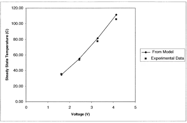
From these results, we were able to take the steady state temperature of the heater at each voltage level and compare it to the results from the model using Equation 2-16. This comparison is shown in Figure 2-7.

120.00- 100.00- 80.00-CU E .-- From Model S60.00-n Experimental Data > 40.00- 2 0.00-0 1 2 3 4 5 Voltage (V)

Figure 2-7 Comparison of steady state temperature of heater obtained from data and from the lumped thermal model. This data is taken from the results of heater testing in Figure 2-6.

From this comparison of the model to the experimental data, we can conclude that the lumped thermal model is adequate to predict the steady state temperature of the heater. Using equation 2-15, we can calculate the time constant of the system for V=3.28 Volts as t=13.3 milliseconds. From Figure 2-7, we can see that this approximates the experimental data, but is a bit slower.

2.2.3 Finite Difference Models

Steady state two-dimensional thermal finite difference models were created in MATLAB in order to predict the temperature distribution along the heater for the two

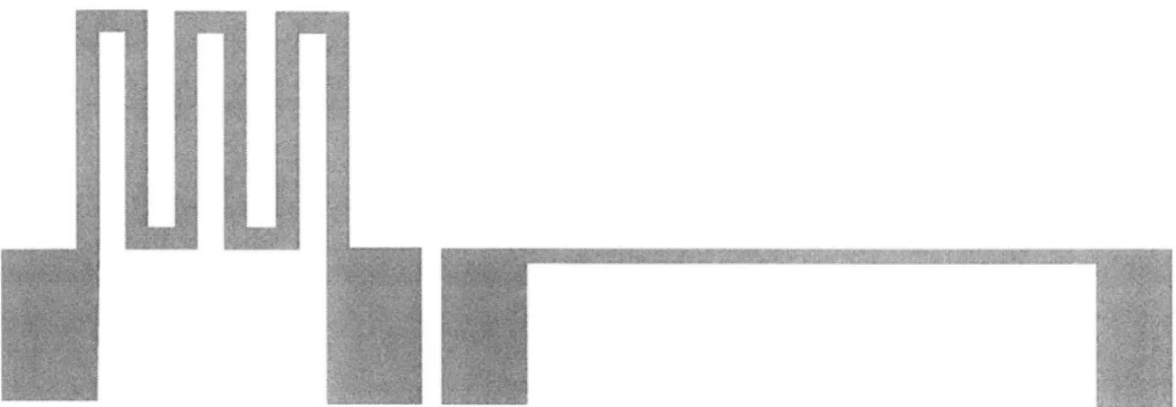
resistor geometries tested. The first generation heater geometry was a straight line heater, while the second generation heater was a folded line resistor (Figure 2-8). By knowing

the temperature distribution along each heater, we can estimate the bubble formation temperature for a particular location on the heater, since only the average heater temperature can be experimentally measured.

Figure 2-8 Two resistor geometries modeled. On the left is the folded resistor, and on the right is the line resistor.

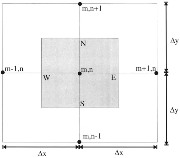
The finite difference model was constructed by breaking each geometry into many smaller control volumes, and then using conservation of energy on each piece. A sample control volume is shown in Figure 2-9.

m,n+1

m+l,n

m-1,n

mn-I

Ax

Ax

Figure 2-9 Sample control volume for finite difference model.

The energy balance on this volume can be written as:

Q=4x

QxI =-k Ay-1=-k mn Ay -k a Ay -I= -k Tmln-Tm,n AY S Ex Ax BT Tmi, -T xS =-k T m-=-k " "Tm'nI Ax ay s _Ay A

Ay

Ay

f

I

aT1 T .,-T

N =-k- _{Ax 1= -k} "'' "' Ax (2-21)

N NAy

AOV = 0' AxAy -1 (2-22)

For the line resistor, the meshed schematic with boundary conditions is shown in Figure 2-10. Each square is 5pmx5gm, and an adiabatic line of symmetry is used in the center of the heater. The resistor is 200ptm long and 10pm wide. The distance from the heater to the ambient temperature boundary condition is 20plm and was determined by estimating the penetration depth of the heat into the quartz for a 50 millisecond time as shown below (the relevant experimental data uses time less than or equal to 50ms):

L ~ ra = 16pm (2-23)

Where L is the penetration depth, r is the time of 5Omsec, and o is the thermal diffusivity of the quartz of 5.27x10-6 m2/sec. For the purpose of the model, L=20pim was chosen as a conservative estimate.

T=300K

-T=300K

T=300K

Figure 2-10 Meshed finite difference model of line heater.

The results of this simulation are shown in Figure 2-11. It is important to note that while the model is able to predict the temperature distribution along the heater, it

neglects conduction in the third dimension and thus cannot accurately predict the actual magnitude of the temperature. The MATLAB code for this model is in Appendix D.

15000---10000 N E 5000--0 6 4 1.5 2 ~ 0.5 X 10-y (M) 0 0(M)

Figure 2-11 Finite difference model temperature distribution results.

The schematic of the folded resistor model with boundary conditions is shown in Figure 2-12. Once again, we use an adiabatic line of symmetry through the center of the heater. As with the model above, the squares are 5gmx5pm, and the penetration depth is L=20pm. The resistor, when unfolded, is 650ptm long and 10ptm wide. The MATLAB code for this model is in Appendix E.

T=300K

T=300K

T=300K

Figure 2-12 Schematic and boundary conditions for folded resistor model.

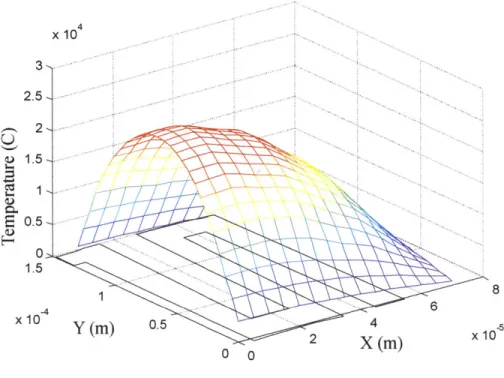
The results of the finite difference simulation are shown in Figure 2-13. It is important to note that there is significantly more temperature variation along the length of the folded heater than along the straight heater.

7 11

I

111]

I III

I

x 104 3 2-1 0.5--1.5 8 -4 . ... 6 x10 Y(m) _{0.5 4-5} 2 X (m) xl

Figure 2-13 Results of finite difference simulation for the folded resistor.

In order to make the simulation results more applicable to the experimental data, the simulations were used to calculate the temperature at various points on the heaters as functions of the average heater temperature. This was chosen because the average heater temperature is the only quantity that may be experimentally measured. These results are shown in Table 2-2.

Heater Geometry Position Percentage Difference from Average Temperature

Straight Center +7.9%

Straight 50pm from Edge +7.7%

Straight Right Edge -47.6%

Folded Center +44%

Folded Top Edge -12%

Folded Bottom Edge -17%

Folded Right Edge -15%

For the straight heaters, because bubbles usually form in the center 100pm of the heater, we can see that the temperature distribution is quite uniform, and near the average heater temperature. Conversely, for the folded heater, we can see that it is important to know where the bubble forms since the temperature distribution is much less uniform. Thus, inferring the temperature of bubble formation will require consideration of the position of bubble formation.

2.3 Bubble Collapse

In the previous chapter, we saw that complete bubble collapse is crucial to the operation of a bubble-powered device, however, many groups have had difficulty accomplishing this. At equilibrium, a small amount of air is dissolved in water, and the solubility of air in water decreases as the temperature of the liquid increases.

Accordingly, when water is boiled, some of the dissolved air comes out of solution and diffuses into the vapor bubble. Because the bubble is no longer filled completely with vapor, the bubble collapse could be limited by both heat transfer/phase change and gas diffusion. In the following sections we will explore both of these bubble collapse mechanisms, and perform order of magnitude estimations of bubble collapse time in the limiting cases of a vapor bubble or an air bubble.

2.3.1 Phase Change Collapse

In this section, we will calculate the time it will take for a 40 tm diameter bubble, filed entirely with water vapor, to condense completely into the surrounding water. In order to solve for this time, we will use the relations derived by Mikic and

Rohsenow[61].

The parameters are defined as follows:

Tb = bulk fluid temperature = 300K Tsat = saturation temperature = 373K

T= wall temperature = 411K

IXwater = thermal diffusivity of water (evaluated at 373K) = 1.69x10-7m2/s rmax = maximum bubble radius = 20ptm

tw = waiting time (time before bubble forms)

c = specific heat of water (evaluated at T=373K) = 4212J/kgK Ja = Jakob Number

pi = density of liquid water (evaluated at T=373K) = 958kg/m3 PV = density of vapor (evaluated at T=373K) = 0.5977kg/m3

tmax = time at which bubble has reached maximum size

tfull = total bubble growth and collapse time

The expression for the bubble radius as a function of time that was derived in the paper can be used to calculate bubble growth time and collapse time. The differential equation for the bubble radius as a function of time is given as:

dr k3 T, -Tat T, -Tb (2-24)

dt ph Sat if rla(t +tj

We can now set dr/dt=0 to solve for tmax, the time it takes for the bubble to reach its maximum size.

t max = Tat )2 2 _(2-25)

_ (T-T't )

K- Tb )2 T vt) The expression for the bubble radius as a function of time is:

2 -j T -T) b t

r I 1 - 1 t (2-26)

)T TW - TCt t t

The Jakob number may be computed as follows:

Ja= , - Ta )C" - 113.48 (2-27)

hfg A

We can use iteration in order to find the proper combination of tw and tmax to achieve rmax=20ptm, using Equations (2-25) and (2-26). In this way we find that tw=1.54x106 s and tmax= 2x 10-7. Now we can solve for the total bubble growth and collapse time, tfulI, by setting r=0 in Equation (2-26), and use this to find the bubble collapse time, tcollapse.

tf,11 = 9.1x10-7 s - t col,,s = t fl -t =7.1x10-7 s (2-28)

In summary, we have been able to estimate the collapse time of a 40gm diameter bubble filled entirely with vapor as being 0.7pts, which can serve as the lower limit for bubble

milliseconds in practice, that the collapse time must begin after the heater is turned off. Hence, from the point of bubble formation, the time it takes for the bubble to collapse is on the order of 50 milliseconds, since the cooling time is similar to the heating time.

2.3.2 Diffusion Collapse

For the case when the bubble is filled completely with air, we will calculate the amount of time it would take for a 40pm diameter bubble to diffuse completely into the surrounding water. For this calculation, we will assume an infinite amount of water surrounding the bubble with no air far from the bubble.

The parameters are defined as follows:

rm = mass transfer rate of air from bubble to water hm= mass transfer coefficient

A = surface area of spherical bubble = nD2

Ac = concentration difference of air between right outside the bubble and at infinity pg= density of air at I atm of pressure and T=300K = 1.177kg/m3

CHe = Henry constant for air in water = 74000 Heair= Henry number for air in water

xair,u = mole fraction of air in water just outside bubble

Xair,s = mole fraction of air just inside bubble = I (assume pure air in bubble) r,= initial bubble radius = 20pm = D/2

D12= diffusion coefficient of air into water

Sc = Schmidt number for air in water at T=300K = 323

g = dynamic viscosity of water at T=300K = 8.67x10-4kg/ms pw = density of water at T=300K = 996kg/m3

The mass transfer relation can be written as:

rh = h1 AAc = hm fD2 Ac (2-29)

The mass transfer may be modeled as quasistatic, which is analogous to heat conduction. Using this analogy between heat transfer and mass transfer, the Nusselt Number for conduction from a sphere may be written as follows for this mass transfer case[62]:

hD= 2 (2-30)

Dn