HAL Id: hal-01443392
https://hal.archives-ouvertes.fr/hal-01443392
Submitted on 23 Jan 2017
HAL is a multi-disciplinary open access
archive for the deposit and dissemination of
sci-entific research documents, whether they are
pub-lished or not. The documents may come from
teaching and research institutions in France or
L’archive ouverte pluridisciplinaire HAL, est
destinée au dépôt et à la diffusion de documents
scientifiques de niveau recherche, publiés ou non,
émanant des établissements d’enseignement et de
recherche français ou étrangers, des laboratoires
FEM-BEM coupling methods for tokamak plasma
axisymmetric free-boundary equilibrium computations
in unbounded domains
Blaise Faugeras, Holger Heumann
To cite this version:
Blaise Faugeras, Holger Heumann. FEM-BEM coupling methods for tokamak plasma axisymmetric
free-boundary equilibrium computations in unbounded domains. [Research Report] RR-9016, INRIA
Sophia Antipolis - Méditerranée; CASTOR. 2017. �hal-01443392�
0249-6399 ISRN INRIA/RR--9016--FR+ENG
RESEARCH
REPORT
N° 9016
Janvier 2017FEM-BEM coupling
methods for tokamak
plasma axisymmetric
free-boundary
equilibrium computations
in unbounded domains
RESEARCH CENTRE
SOPHIA ANTIPOLIS – MÉDITERRANÉE
2004 route des Lucioles - BP 93
FEM-BEM coupling methods for tokamak
plasma axisymmetric free-boundary
equilibrium computations in unbounded
domains
Blaise Faugeras, Holger Heumann
Project-Teams CASTOR
Research Report n° 9016 — Janvier 2017 — 2 pages
Abstract: Incorporating boundary conditions at infinity into simulations on bounded com-putational domains is a repeatedly occurring problem in scientific computing. The combination of finite element methods (FEM) and boundary element methods (BEM) is the obvious instru-ment, and we adapt here for the first time the two standard FEM-BEM coupling approaches to the free-boundary equilibrium problem: the Johnson-N´ed´elec coupling and the Bielak-MacCamy coupling. We recall also the classical approach for fusion applications, dubbed according to its first appearance von-Hagenow-Lackner coupling and present the less used alternative introduced in [AlbaneseEtAL1986]. These methods are compared through numerical experiments. We show that the von-Hagenow-Lackner coupling su↵ers from non-optimal approximations properties, and, moreover, that such coupling methods require Newton-like iteration schemes, for solving the cor-responding non-linear discrete algebraic systems.
R´esum´e : La prise en compte des conditions aux limites `a l’infini dans les sim-ulations sur des domaines de calcul born´es est un probl`eme r´ecurrent en calcul scientifique. Pour ce faire le couplage de la m´ethode des ´el´ements finis (FEM) avec celle des ´el´ements de fronti`ere (BEM) est l’outil naturel. Nous adaptons ici pour la premi`ere fois les deux approches standards de couplage FEM-BEM pour le probl`eme de l’´equilibre du plasma: le couplage de Johnson-N´ed´elec et celui de Bielak-MacCamy. Nous rappelons ´egalement l’approche classique dans les codes de fusion, baptis´ee selon sa premi`ere apparition couplage de von-Hagenow-Lackner et pr´esentons l’alternative moins utilis´ee introduite dans [AlbaneseE-tAL1986]. Ces m´ethodes sont compar´ees au travers d’exp´eriences num´eriques. Nous montrons que le couplage von-Hagenow-Lackner sou↵re d’une conver-gence non-optimale et, en outre, que de telles m´ethodes de couplage n´ecessitent l’utilisation de sch´emas it´eratifs de type Newton, pour r´esoudre les syst`emes alg´ebriques discrets non lin´eaires correspondants.
Mots-cl´es : couplage FEM-BEM; d’´equilibres axisym´etriques `a fronti`ere libre d’un plasma de tokamak
FEM-BEM coupling methods for tokamak plasma
axisymmetric free-boundary equilibrium computations
in unbounded domains
Blaise Faugeras, Holger Heumann1
CASTOR Team, INRIA Sophia-Antipolis and Universit´e de Nice Parc Valrose, 06108 Nice cedex 02, FR
Abstract
Incorporating boundary conditions at infinity into simulations on bounded com-putational domains is a repeatedly occurring problem in scientific computing. The combination of finite element methods (FEM) and boundary element meth-ods (BEM) is the obvious instrument, and we adapt here for the first time the two standard FEM-BEM coupling approaches to the free-boundary equilibrium problem: the Johnson-N´ed´elec coupling and the Bielak-MacCamy coupling. We recall also the classical approach for fusion applications, dubbed according to its first appearance von-Hagenow-Lackner coupling and present the less used al-ternative introduced in [2]. These methods are compared through numerical ex-periments. We show that the von-Hagenow-Lackner coupling su↵ers from non-optimal approximations properties, and, moreover, that such coupling methods require Newton-like iteration schemes, for solving the corresponding non-linear discrete algebraic systems.
Keywords:
Note: Some figures in this paper are in color only in the electronic version.
1. Introduction
Numerical equilibrium computation is undoubtedly of first importance in Tokamak fusion science [38] and has been studied for a long time with already a review article in 1991 [37]. From a Tokamak operation point of view equilibrium codes are essential to design the geometry of new machines, to set up discharge scenarios and to check their feasibility, or to design and validate plasma feed-back controllers. To this end these 2D equilibrium codes can also be coupled to 1D transport codes in order to simulate the evolution of the plasma equilibrium
Email addresses: [email protected] (Blaise Faugeras), [email protected](Holger Heumann)
at the di↵usion timescale through out the discharge [20]. More detailed mag-netohydrodynamic simulations modeling the plasma on very short timescales also rely on a given initial equilibrium which is the output of these equilibrium codes. As a last example let us mention that equilibrium computation methods are also used in equilibrium reconstruction codes which aim at identifying the toroidal current density in the plasma from experimental measurements (e.g. [30, 31, 7, 8, 32]).
A code which treats the quasi-static free-boundary equilibrium problem needs to solve nonlinear elliptic or parabolic problems with nonlinear source terms representing the current density profile vanishing outside the unknown free boundary of the plasma. The computational challenges in the design of such a code are: a problem setting in an unbounded domain with a nonlinear-ity due to the current densnonlinear-ity profile in the unknown plasma domain and the nonlinear magnetic permeability if the machine has ferromagnetic structures.
In this paper we focus on how the simulation on the unbounded domain can be reduced to computations on an interior bounded domain thanks to analytical Green’s functions [29]. The numerical solution on the interior domain is coupled through boundary conditions to the Green’s function representation of the solu-tion in the unbounded exterior domain. This approach is today fairly standard in many other application areas such as electromagnetics [21, 39, 4] or elastic-ity [12, 5, 36] and falls in the framework of boundary integral equations. The boundary integrals equations enable to reduce problems on unbounded domains to problems on boundaries which can then be coupled to any numerical method for the interior bounded domain. Most authors in the fusion literature deal with this question using a method introduced by von Hagenow and Lackner [18, 29], whereas the coupling could be also conceived in other ways. In this paper our goal is to compare four di↵erent schemes in order to assess their performance.
As aforementioned, certainly the most famous coupling in the fusion commu-nity is called in this paper the von Hagenow-Lackner coupling HLC [18, 29]. A method implementing this coupling is present in many equilibrium codes which usually make use of a finite di↵erence discretization method and of fixed-point iterations to solve the nonlinearities. Here we propose a variational framework for this coupling which enables the use of a finite element method (FEM) com-bined with a boundary element method (BEM) and Newton method for the nonlinearities. Surprisingly this method does not seem to be known in the applied mathematics or scientific computing literature.
Much less known and used but nevertheless existing in the fusion literature is the analytic uncoupling on a semi-circular domain AUC introduced in Albanese, Blum and Barbieri [2]. It is the method implemented in the codes Proteus [3], and the more recent CREATE-NL+ [1] or CEDRES++ and FEEQS.M [17, 19]. Such an uncoupling method was also analysed for the case of the Laplacian operator in [22] and [15].
The two other methods we will discuss in this work are very well known in the applied mathematics literature and often referred to as the Johnson-N´ed´elec coupling JNC [40, 27, 34] and the Bielak-MacCamy coupling BMC [5]. From our point of view JNC might be the most natural way to deal with the unbounded
domain problem in the framework of a finite element method. However, neither JNC nor BMC have never been tested before in a fusion equilibrium code.
The outline of the paper is the following. In Section 2 we recall the plasma equilibrium equations in a Tokamak and present afterwards in Section 3 the boundary integral equations and the di↵erent coupling methods. Section 4 deals with the Galerkin formulations leading to the FEM-BEM discretizations of the four di↵erent coupling methods. Numerical experiments are conducted in Sec-tion 5 and we conclude with a short summary and outlook in SecSec-tion 6. 2. Equilibrium equation
We consider the magnetostatic problem curl ✓ 1 µcurl A ◆ = J
of the electromagnetic vector potential A for some given current density J with µ the permeability. Under the axisymmetry assumption it is rewritten in cylin-drical coordinates x = (xr, xz) r · ✓ 1 µ0xrr (x) ◆ = J(x)· e'; (0, xz) = 0 ; lim kxk!+1 (x) = 0 ; (1)
wherer is the gradient in the two dimensions (xr, xz). The primal unknown
is the poloidal magnetic flux (x) := xrA(x)·e', the scaled toroidal component
of the vector potential A, i.e. B = curl A and e' the unit vector in toroidal
direction. We consider air transformer tokamaks only, that is to say that the permeability is the constant µ0everywhere and the non-linearities are only due
to the plasma domain and current density. In the here considered free boundary equilibrium problem the toroidal component of the current density is given by
J(x)· e'= 8 > < > : j(xr, (x)) in P ( ) ; jci in Ci; 0 elsewhere , (2)
with jci = Ii/|Ci| is the given constant current density in the i-th poloidal field coil Ci ⇢ ⌦1= [0,1] ⇥ [ 1, 1] and j(xr, (x)) the prescribed toroidal
component of the plasma current density, generally a non-linear function of , in the plasma domain P ( )⇢ ⌦L⇢ ⌦1 with ⌦L the limiter domain accessible
to the plasma. The plasma domain P ( ) is the domain bounded by the last closed poloidal flux line inside the limiter domain. Hence the axisymmetric magnetostatic problem is a non-linear problem, which, due to the unknown plasma domain P ( ) is called the free-boundary equilibrium problem. We refer to standard text books (e.g. [14, 6, 38, 16, 26]) for further details on the derivation of this modelization.
3. Boundary integral coupling methods
To solve problem (1) numerically we need to find a reformulation on a bounded domain ⌦b, the computational domain, containing the plasma domain
P ( ), where the coupling with the solution on the complement ⌦e = ⌦1\ ⌦b
is ensured by appropriate boundary conditions. The boundary conditions are given by boundary integral equations that follow from Green’s identities.
If not stated di↵erently, we are not assuming that the computational domain ⌦b contains all the coils and hence we introduce the two index subsets Ib =
{i / Ci⇢ ⌦b} and Ie={i / Ci⇢ ⌦e} to distinguish coils in ⌦band coils in ⌦e.
Boundary integral equations. The methods investigated in this work rely on Green’s theorem for the di↵erential operatorr·⇣ 1
µ0xrr· ⌘
noted ⇤. Namely
for any domain D⇢ ⌦1 and all regular enough and ⇠ it holds that (see e.g.
[35, page 1-3, eq. 1.8] or [24, page 428]) Z
D
( (y) ⇤⇠(y) ⇠(y) ⇤ (y))dy+ Z
@D
(@⇤n(y) (y)⇠(y) @n(y)⇤ ⇠(y) (y))ds(y) = 0 , (3)
where y = (yr, yz), n is the outward normal vector on @D and @n⇤⇠(x) = 1
µ0xrr⇠(x) · n.
Let us also introduce the fundamental solution of ⇤ [25] which writes
explicitly as
G(x, y) = µ0 px
ryr
2⇡k(x, y) (2 k
2(x, y))K(k(x, y)) 2E(k(x, y)) ,
with
k2(x, y) = 4xryr
(xr+ yr)2+ (xz yz)2,
and K(k) and E(k) are the complete elliptic integrals of the first and second kind respectively. Hence, taking in (3) (y) = G(x, y) we have the integral identity (see e.g. [35, page 89, eq. 5.2] or [24, eq. 9]) in D:
⇠(x) + Z @D @n(y)⇤ G(x, y)⇠(y)ds(y) Z @D
@n(y)⇤ ⇠(y)G(x, y)ds(y)
= Z
D
G(x, y) ⇤⇠(y)dy 8x 2 D (4) for all regular enough ⇠. Further, it can be shown (see e.g. [35, page 137, eq. 6.20,] or [24, eq. 11]) that in the limit x2 @D the following integral identity holds: 1 2⇠(x) + Z @D @n(y)⇤ G(x, y)⇠(y)ds(y) Z @D
@n(y)⇤ ⇠(y)G(x, y)ds(y)
= Z
D
von Hagenow-Lackner coupling HLC [18, 29]. No specific shape is as-sumed for ⌦b which is not necessarily connected. Green’s second identity (3)
for D = ⌦1 with = G and ⇠ = the solution of (1) leads to a non-linear
integral equation for : (x) =
Z
P ( )
j(yr, (y))G(x, y)dy +
X
i2Ib[Ie Z
Ci
jciG(x, y)dy 8x 2 ⌦1. (6)
In particular this provides a formula for the Dirichlet conditions of on the boundary @⌦b of the computational domain. Hence it is possible to
reformu-late the free-boundary equilibrium problem in the unbounded domain (1) as a Dirichlet boundary value problem in the bounded domain ⌦b using expression
(6) as the Dirichlet boundary condition.
In order to avoid the computation of the integral over the possible large domain P ( ) when evaluating (6), one then introduces a new auxiliary unknown u satisfying the homogeneous Dirichlet boundary value problem
⇤u(x) = j(x
r, ) P ( )(x) +
X
i2Ib
jci Ci(x) in ⌦b, u = 0 on @⌦b, (7) where is the domain indicator function. Green’s third identity (5) for D = ⌦b
with ⇠ = u leads to Z
P ( )
j(yr, (y))G(x, y)dy +
X i2I Z Ci jciG(x, y)dy = Z @⌦b
@⇤n(y)u(y)G(x, y)ds(y) 8x 2 @⌦b, (8)
with n(y) the inward pointing normal of ⌦b, showing that the integral over
plasma domain and coils in ⌦ in equation (6) can be replaced by an integral over the boundary @⌦b using the Neumann data of u, the solution to problem
(7). Hence the Dirichlet boundary condition on @⌦b is expressed as the sum
of the boundary integral in (8) involving the new unknown u and the Green function convolutions term of the currents flowing in ⌦e.
Johnson-N´ed´el´ec coupling JNC, direct method [40, 27]. As for HLC here no specific shape is assumed for ⌦b which is not necessarily connected.
One introduces a supplementary unknown q⇡ @⇤
n for the Neumann boundary
condition on @⌦b, where n is the inward pointing normal of ⌦b. Green’s third
identity (5) for in ⌦e gives a supplementary boundary integral equation:
1 2 (x) +
Z
@⌦b
(@⇤n(y)G(x, y) (y) q(y)G(x, y))ds(y)
=X
i2Ie Z
Ci
jciG(x, y)dy 8x 2 @⌦b. (9)
So, JNC amounts to couple the Neumann problem for in ⌦bwith the integral
Bielak-MacCamy coupling BMC, indirect method [5]. As for HLC and JNC here no specific shape is assumed for ⌦bwhich is not necessarily connected.
One introduces a supplementary unknown potential q on @⌦b, and defines an
auxiliary unknown ⇠(x) for x 2 ⌦e, based on a boundary integral over the
potential q ⇠(x) := Z @⌦b G(x, y)q(y)ds(y) +X i2Ie Z Ci jciG(x, y)dy , (10)
and finds, again by Green’s theorem, that
⇤⇠(x) =X i2Ie Z
Ci
jciG(x, y)dy in ⌦e,
meaning that ⇠(x) is a representation of the solution (x) of (1) when x2 ⌦e.
In the limit cases x 2 @⌦b we get integral representation formulas for the
Dirichlet trace of ⇠ ⇠(x) = Z @⌦b G(x, y)q(y)ds(y) +X i2Ie Z Ci jciG(x, y)dy , (11)
and the Neumann trace of ⇠ @⇤n⇠(x) = 1 2q(x) + Z @⌦b @n(x)⇤ G(x, y)q(y)ds(y) +X i2Ie Z Ci jci@ ⇤ n(x)G(x, y)dy x2 @⌦b, (12)
which are forced to be equal to the Dirichlet and Neumann trace of . Here again n is the inward pointing normal of ⌦b. Hence, BMC amounts to combine the
Neumann problem for in ⌦b, based on q-parametrized Neumann data given
by the right hand side of (12), with the integral equation (11) that involves as well (through its Dirichlet trace) and the potential q.
Analytic uncoupling on a semi-circular domain AUC [2] [15]. Let us choose ⌦b to be a semi-circular domain containing ⌦L and all the coils Ci.
Its boundary is @⌦b = [ 0 where is the semi-circle of radius ⇢ and 0={(0, z) / ⇢ z ⇢ }. This particular choice enables to find
analyti-cally, thanks to the method of images, a special Green function G⇤(x, y) which vanishes on the semi-circle . Then using Green’s theorem (3) with D = ⌦e
and = G⇤ one obtains
(x) = Z
(y)@n(y)⇤ G⇤(x, y)ds(y) 8x 2 . (13)
The normal derivative @⇤
n (x) can then also be analytically computed as a
boundary integral depending on and reinjected in the boundary condition term of the variational formulation for the inner problem on ⌦b. We refer to
4. Galerkin formulation
In most of the computational tools for computing axisymmetric plasma equi-libria the finite di↵erence method for the strong formulation (1) of the equilib-rium problem is combined with the HLC. We follow here the more general Galerkin method, and recall that for appropriately chosen triangulations the Galerkin method leads to the same stencils as the finite di↵erence approach. Moreover the Galerkin method allows more flexibility for approximating the realistic geometry of a tokamak.
We consider problem (1) restricted to the bounded computational domain ⌦b, multiply by a test function ⇠ and do integration by parts:
Z ⌦b 1 µ0xrr (x) · r⇠(x) dx + Z @⌦b @n⇤ (x) ⇠(x) ds(x) = Z ⌦b J(x)· e'⇠(x) dx , (14) where n is the inward pointing normal.
We use a triangular mesh to cover the computational domain ⌦band
intro-duce a basis of piecewise linear functions{ i}, where each ivanish at all mesh
vertices except one. Basis functions associated to vertices at xr= 0 are excluded
from this finite element space X(⌦b), as, due to axisymmetry (0, xz) = 0. The
finite element space X(⌦b), is the linear Lagrangian finite element space and
has the direct decomposition X(⌦b) = X (⌦b) X@(⌦b), where X (⌦b) is the
space of all finite element functions in X(⌦b) that have zero Dirichlet trace. The
degrees of freedom of elements of X (⌦b) are the values at the vertices of the
mesh, that are not on the boundary @⌦band the degrees of freedom of elements
of X@(⌦b) are the values at the vertices on the boundary @⌦b . Additionally
we will make use of the finite element space Q(⌦b) being the span of piecewise
constant functions{ i}, where each i vanishes everywhere except for one edge
of the boundary @⌦b.
To define the di↵erent Galerkin formulations of HLC, JNC, BMC and AUC let us introduce the following notations for operators related to the Galerkin method on ⌦b: a( , ⇠) := Z ⌦b 1 µ0xrr (x) · r⇠(x)dx , jp ( , ⇠) := Z P ( ) j(xr, (x))⇠(x)dx (15) and `(⇠) :=X i2Ib jci Z Ci ⇠(x)dx . (16)
The implementation of these operators relies on quadrature rules for integrals over the triangular elements of the mesh. The approximation of the non-linear jp( , ⇠) is non-standard due to the integration domain depending on and
Moreover we will make also use of boundary integral operators and introduce V (q)(x) := Z @⌦b G(x, y)q(y)ds(y) , x2 @⌦b, K( )(x) := Z @⌦b @n(y)⇤ G(x, y) (y)ds(y) , x2 @⌦b, K0( )(x) := Z @⌦b @n(x)⇤ G(x, y) (y)ds(y) , x2 @⌦b, (17)
and domain integral operators L(x) :=X i2Ie jci Z Ci G(x, y)dy , x2 ⌦b, L0(x) =X i2Ie jci Z Ci @n(x)⇤ G(x, y)dy , x2 ⌦b. (18)
In the subsequent Galerkin formulations we will frequently integrate products of integral operators and test functions over the boundary, hence it is convenient to introduce also
h , ⇠i@⌦b:= Z
@⌦b
(x) ⇠(x)ds(x) . (19)
In the case where is one of the boundary integral operator in (17) the ap-proximation of such inner products is non-trivial and goes beyond the standard quadrature formulas. Nevertheless, this task is well understood, and we refer to [11] for the technical details recalling also the asymptotic formulas for the fundamental solution G(x, y) whenkx yk ! 0 derived in [23].
In the subsequent text we will distinguish between the computational domain ⌦b = ⌦ that verifies the assumptions for HLC, JNC, BMC and the
computa-tional domain ⌦b= ⌦H# that verifies the assumptions for AUC. While ⌦H# is a
semi-circular domain containing ⌦L and all the coils Ci, the domain ⌦ only
re-quires to contain ⌦L, the domain that is accessible by the plasma. In particular
it is not required that ⌦ is a connected domain.
HLC, ⌦b= ⌦. Dirichlet boundary conditions g are imposed in (14) and
com-puted using equations (6), (7) and (8). This leads to the introduction of the following Galerkin formulation: find ( , g, u)2 X (⌦) ⇥ X@(⌦)⇥ X (⌦), such
that
a( , ⇠) + a(g, ⇠) jp( , ⇠) = `(⇠) , 8⇠ 2 X (⌦) ,
hg, fi@⌦ hV (@n⇤u), fi@⌦=hL, fi@⌦, 8f 2 X@(⌦) ,
a(u, v) jp( , v) = `(v) , 8v 2 X (⌦) .
(20)
JNC, ⌦b= ⌦. We supplement equation (14) for on ⌦ with boundary integral
equation (9) for q, the auxiliary variable for the Neumann data, and obtain the following variational formulation: find ( , q)2 X(⌦) ⇥ Q(⌦), such that
a( , ⇠) jp( , ⇠) +hq, ⇠i@⌦= `(⇠) , 8⇠ 2 X(⌦) ,
h12 + K( ), pi@⌦ hV (q), pi@⌦=hL, pi@⌦, 8p 2 Q(⌦) .
BMC, ⌦b = ⌦. We supplement equation (14) for on ⌦ with boundary
integral equation (11), use (12) for the Neumann data and obtain the following variational formulation: find ( , q)2 X(⌦) ⇥ Q(⌦), such that
a( , ⇠) jp( , ⇠) +h 1 2q + K 0(q), ⇠i @⌦= `(⇠) hL0, ⇠i@⌦, 8⇠ 2 X(⌦) , h , pi@⌦ hV (q), pi@⌦=hL, pi@⌦, 8p 2 Q(⌦) . (22)
AUC, ⌦b= ⌦H# . The variational formulation for this method is given in [19].
We briefly recall it here for completeness: Find 2 X(⌦H#) such that
a( , ⇠) jp( , ⇠) + c( , ⇠) = `(⇠) 8⇠ 2 X(⌦H#) . (23)
The bilinear form c(·, ·) derives from (13) as detailed in [17]. It is defined as follows c( , ⇠) := 1 µ0 Z (x)N (x)⇠(x)ds(x) + 1 2µ0 Z Z
( (x) (y))M (x, y)(⇠(x) ⇠(y))ds(x)ds(y) , (24) with M (x, y) = k(x, y) 2⇡(xryr) 3 2 ✓ 2 k(x, y)2
2 2k(x, y)2E(k(x, y)) K(k(x, y))
◆ , N (x) = 1 xr ✓ 1 + + 1 1 ⇢ ◆ and ± = p x2 r+ (⇢ ± xz)2,
where ⇢ is the radius of the circle defining ⌦H#.
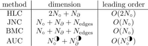
Each of the four Galerkin formulations corresponds to a finite dimensional non-linear system F(U) = 0, where we provide the di↵erent dimensions in Table 1. In general we can say that N = dim(X (⌦)), the number of vertices not on the boundary, is orders of magnitude larger than N@ = dim(X@(⌦)) the number
of vertices on the boundary and Nedges = dim(Q(⌦)) the number of edges on
the boundary. Hence, in summary the non-linear algebraic system for HLC will be roughly twice as large as the non-linear algebraic system for JNC and BMC. Moreover, comparing HLC, JNC and BMC with AUC, the requirement of AUC of ⌦H# to be a half circle seems to lead to an undesirable increase of unknowns for AUC.
On the other hand, the ultimate performance of all the four methods is only indirectly linked to the dimension. Due to the non-linearity, we need to employ iteration schemes, and so the performance is more linked to the number of iterations needed to achieve convergence and also to the computational time that is required to update from iteration n to iteration n + 1.
To keep the number of iterations small Newton type methods with their fast superlinear or even quadratic convergence are highly recommended. Newton type methods for AUC are advocated in the numerous contributions, starting
with [9], since the early eighties. Without any additional technicality it is also possible to use Newton’s method for the other three di↵erent formulations. The only non-trivial term in the derivative of each F, corresponds to the derivative of jp( , ⇠), that can be found in [19] where it was introduced for the coupling
approach AUC. All the codes that implement HLC so far are using Picard type iterations that avoid the derivative of jp( , ⇠). The original approach [29] reads
as: Given ( n, gn)2 X (⌦)⇥X@(⌦) find ( n+1, gn+1, un+1)2 X (⌦)⇥X@(⌦)⇥
X (⌦) such that a( n+1, ⇠) + a(gn, ⇠) jp( n, ⇠) = `(⇠) , 8⇠ 2 X (⌦) , hgn+1, fi@⌦ hV (@n⇤un+1), fi@⌦=hL, fi@⌦, 8f 2 X@(⌦) , a(un+1, v) j p( n+1, v) = `(v) , 8v 2 X (⌦) , (25)
which has the advantage that one needs to solve in each iteration only two Dirichlet problems for the linear operator ⇤. It is possible to derive highly efficent algorithms for this task combining finite di↵erences and fast Fourier transform. Nevertheless, it is reported that such iteration schemes su↵er from serious convergence problems [29, 26] and in [6] it was shown that Picard type iterations for AUC can lead to non-converging schemes.
In efficient implementations of either Newton or Picard type schemes for HLC, JNC, BMC or AUC the most time consuming part of each update will be the inversion of large linear systems. Here it is a priori not clear whether a Newton type scheme for JNC and BMC is superior to a Newton type scheme for AUC: the linear systems of JNC and BMC are considerable smaller than the linear systems for AUC, but the integral equations in JNC and BMC lead to dense entries in the linear system, which can demand large resources for the inversion.
Newton-type iterations are known to converge super-linearly, once the iterate is sufficiently close to the solution. But as it is not easy to quantify ”sufficiently close”, one generally needs to invokes so called globalization strategies. For the moment, we exclude such globalization strategies from our discussions, but assume that we have a sufficiently good initial guess. This is indeed the case in many applications, e.g. equilibrium reconstructions, where the equilibrium at the previous timestep is a good initial guess, or scenario development, where the formulation of inverse problems allows to find coil current that correspond to a prescribed equilibrium.
5. Numerical experiments
All the subsequent simulations and numerical experiments were performed on a MacBook Pro with the 2,8 GHz Intel Core i7 processor and 16 GB 1600 MHz DDR3 memory. The implementation is basically an extension of FEEQS.M2,
which is a MATLAB implementation of the methods for axisymmetric free
method dimension leading order
HLC 2N + N@ O(2N )
JNC N + N@+ Nedges O(N )
BMC N + N@+ Nedges O(N )
AUC N H# + NH@# O(N H#)
Table 1: The dimensions of the finite dimensional non-linear system F(U) = 0 for the four di↵erent methods. N = dim(X (⌦)) and N H# = dim(X (⌦H#)) is the number of vertices not on the boundary, N@= dim(X@(⌦)) and N H@#= dim(X@(⌦H#)) is the number of vertices on
the boundary and Nedges = dim(Q) is the number of edges on the boundary. We use the
superscript H# to recall that AUC requires the computational domain to be a half circle ⌦H#. In general N ⌧ N@.
boundary plasma equilibria that are described in [19]. Concerning, the details of the implementation, e.g. quadrature rules and the accurate linearizations of various terms in the Galerkin formulations (20), (21), (22) and (23), we refer to [19] and [11]. The code utilizes in large parts vectorization, and therefore, the running time is comparable to C/C++ implementations (see [28, 10] and [13] for a review and earlier references). FEEQS.M is publicly available and a forth-coming release will contain the here introduced coupling methods for plasma equilibrium calculations.
5.1. Convergence
We solve a simple magnetostatic problem in axial symmetry, which corre-sponds to a constant current carrying coil with poloidal section C = [0.5, 1.5]⇥ [ 1.5, 0.5]: r · ✓ 1 µ0rr ◆ = ( 1 in C ; 0 elsewhere , (0, z) = 0 ; lim k(r,z)k!+1 (r, z) = 0 . (26)
With this simple linear test problem we can easily assess numerically the ap-proximation quality of the four di↵erent approaches. The solution of (26) and its gradientr in ⌦1\ C are
(x) = Z C G(x, y)dy , r (x) = Z Cr xG(x, y)dy . (27)
To study the convergence behavior of the di↵erent coupling approaches we in-troduce a second square D = [1, 2]⇥ [0.5, 1.5]. The approaches HLC, JNC and BMC for solving (26) are based on either the domain ⌦b = ⌦ = D or the
do-main ⌦b = ⌦ = C [ D for the finite element discretization. The first choice
corresponds to the case when no source term are in the computational domain ⌦, while the second choice is more relevant for the equilibrium problem, as it
0 1 2 3 -3 -2 -1 0 1 2 3 0 1 2 3 -3 -2 -1 0 1 2 3 0 1 2 3 -3 -2 -1 0 1 2 3
Figure 1: Center: The domain C (green) and the domain D (yellow). Left: Example of the meshes used in the coupling methods HLC, JNC and BMC. Right: Example of the meshes used for the coupling method AUC.
corresponds to the case when source terms, such as the plasma are in the com-putational domain ⌦. For AUC we always choose ⌦b= ⌦H# to be the half circle
of radius 3 centered at (0, 0) that contains both D and C (see Figure 1 of an illustration). As we consider here the linear problem the term jp( ,·) vanishes
in all four Galerkin formulations (20), (21), (22) and (23). Moreover, in the case of no sources in the computational domain, ⌦ = D, we have that `(·) vanishes while in the case of ⌦ = D\ C both L(x) and L0(x) vanish.
Then we compute the numerical solutions HLC
h , JNCh , hBMC and hAUC
with either of the four methods on a sequence of refined meshes and monitor the error in the domain D measured in the L2-norm and the H1-semi-norm:
errM0 = sZ D ( M h(x) (x))2dx , err M 1 = sZ D|r M h(x) r (x)|2dx ,
where M runs through JNC, HLC, BMC and AUC and we use high precision quadrature for the convolution formulas in (27) to approximate (x) andr (x). The results are shown in Figures 2 and 3.
First (see Figure 2, left), we look at the case when there are no sources in the computational domain. The numerical experiments confirm theoretical convergence assertions [27, 11] for the coupling methods JNC and BMC: as we are using piecewise affine finite elements we observe second and first order convergence in the L2-norm and the H1semi-norm respectively. We are loosing
one order of convergence for BMC in L2, which is due to a loss of regularity
10 2 10 1 100 105 104 103 102 101 100 101 i = 0: HLC JNC BMC O(h2) i = 1: HLC JNC BMC O(h1) h d is cr et e er ror , er r M i 10 2 10 1 100 10 5 10 4 10 3 10 2 10 1 100 101 i = 0: HLC JNC AUC O(h2) i = 1: HLC JNC AUC O(h1) h d is cr et e er ror , er r M i
Figure 2: Left: Without sources in the computational domain, ⌦b= ⌦ = D (not possible for
(AUC)). Right: With sources in the computational domain, ⌦b= ⌦ = D[ C for (HLC) and
(JNC) and ⌦b= ⌦⇤a half circle for (AUC).
10 2 10 1 100 105 104 103 102 101 100 i = 0: LFE-LFE LFE-QFE O(h2) i = 1: LFE-LFE LFE-QFE O(h1) h d is cr et e er ror , er r HLC i 0.5 1 1.5 2 2.5 3 -2 -1.5 -1 -0.5 0 0.5 1 1.5 2 0.5 1 1.5 2 2.5 3 -2 -1.5 -1 -0.5 0 0.5 1 1.5 2
Figure 3: Left: The suboptimal convergence rate for HLCin L2can be improved if we use
quadratic finite elements (LFE-QFE) instead the linear finite elements (LFE-LFE) in (20) for the auxiliary variable u. Right: The computational domain ⌦ and the coarsest mesh, with the subdomains D (yellow), the domain where we evaluate the error and the domain C (green) the support of the source term.
0 5 10 -10 -5 0 5 10 0 5 10 -10 -5 0 5 10 1 2 3 4 5 6 7 8 9 10 11 12 0 5 10 -10 -5 0 5 10
Figure 4: The ITER geometry (center) and the mesh for the domain ⌦H# and the domain ⌦. The coils are not included in ⌦.
149] disadvantage of indirect boundary integral methods such as BMC and we therefore exclude BMC from the subsequent discussion.
To our knowledge there is no theoretical convergence analysis available for HLC. While we see (see Figure 2, left) with ⌦b = ⌦ = D as well first order
convergence in the H1-semi-norm, and second order convergence in the L2
-norm, we observe a loss of convergence for the case that sources are in the FEM domain (see Figure 2, right). This is inherent in the method and a sever disadvantage of HLC. A closer inspection of the last line of (20) shows, that we basically approximate the missing Dirichlet data for by a convolution with the Neumann data of the auxiliary variable u. Since the Neumann data involves the gradient of u, this approximation is of lower order than required in the standard numerical analysis of Dirichlet problems with approximated Dirichlet data. To cure this defect we would have to discretize the auxiliary variable u with at least quadratic finite elements (see Figure 3), which then leads to an increase in the number of unknowns.
In the relevant case of sources in the computational domain, we observe a very similar convergence behavior of AUC and JNC (see Figure 2, left).
In the following subsection we monitor the characteristic running times for each of the three approaches for a realistic equilibrium problem.
5.2. Running time
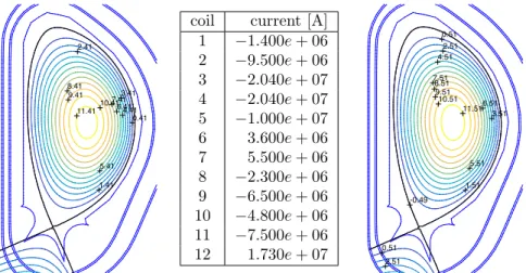
In the following we consider an example for ITER geometry (see Figure 4, center) with the coil currents indicated in the table in Figure 5. The current
11.4110.41 9.41 8.41 7.41 6.41 5.41 4.41 3.41 2.41 1.41 0.41
coil current [A] 1 1.400e + 06 2 9.500e + 06 3 2.040e + 07 4 2.040e + 07 5 1.000e + 07 6 3.600e + 06 7 5.500e + 06 8 2.300e + 06 9 6.500e + 06 10 4.800e + 06 11 7.500e + 06 12 1.730e + 07 11.51 10.51 9.51 8.51 7.51 6.51 5.51 4.51 3.51 2.51 2.51 1.51 0.51 0.51 -0.49
Figure 5: Case A: The currents in the coils (center) and contour plots of numerical solutions using AUC (left) and HLC (right).
profile is the parametric profile j(xr, (x)) = ( xr
r0
+ (1 )r0 xr
)(1 N(x)↵)
with r0 = 6.2m the major radius of the vacuum chamber and ↵ = 2.0, =
0.5978, = 1.395 and = 1.365461e + 6. N the normalized poloidal flux N(x) = (x) ax( )
bd( ) ax( )
,
where ax and bd are the flux values at the magnetic axis and the boundary.
Exemplary meshes for AUC and HLC/JNC are shown in Figure 4. HLC and JNC are based on a mesh that covers the domain bounded by the outer vac-uum vessel wall. The initial guesses are solutions to equilibrium problems with fixed, prescribed plasma current, and then the Newton iterations converge to a residual smaller then 10 12 in less then 10 iterations. The di↵erence between
the numerical solutions of AUC, HLC and JNC is negligible (see Figure 5 left and right), so we can focus on the runtime. As all the three methods are im-plemented in the same environment, this is a fair test to assess the performance of each approach. A more sophisticated implementation that allows to improve the performance of one method, will also improve the performance of the two other methods.
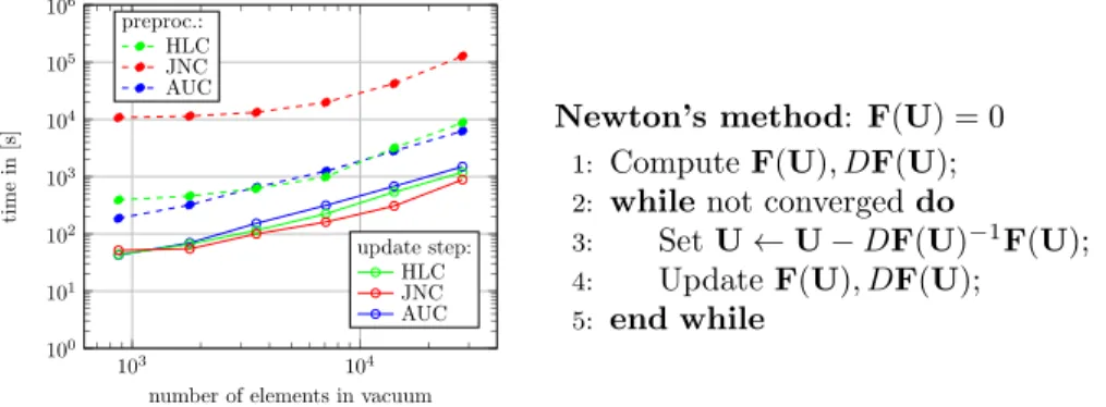
The pseudo-code for Newton-type schemes can be found in Figure 6. In our first test, we look at the timing of the pre-processing, the line 1 in the pseudo-code, and time per Newton iteration, the update step in the lines 3 and 4 in the pseudo-code (see Figure 6). The pre-processing steps consists mainly of the assembling of all sti↵ness matrices that do not change during the Newton iterations. This involves in particular the assembling of all boundary integral terms, that has in general quadratic complexity due to the convolution terms.
103 104 100 101 102 103 104 105 106 preproc.: HLC JNC AUC update step: HLC JNC AUC
number of elements in vacuum
tim
e
in
[s
] Newton’s method: F(U) = 0
1: Compute F(U), DF(U);
2: while not converged do
3: Set U U DF(U) 1F(U);
4: Update F(U), DF(U);
5: end while
Figure 6: Timing of the pre-processing (preproc.), the line 1 in Newton’s method, and time per Newton Iteration (update step), the lines 3 and 4 in Newton’s method, for the di↵erent coupling methods.
The main e↵ort in the update step is due to the inversion of the Newton matrix and due to the update of the plasma domain and its corresponding terms, e.g jp( , ⇠) in the Galerkin formulations. We show in Figure 6 characteristic
tim-ings of the pre-processing step and the update step as functions of the number triangles that cover the domain accessible by the plasma (orange in Figure 4), as this number is identical for both type of meshes. Saying this, it is obvious that the pre-processing time for JNC is the largest, as it contains more bound-ary integral terms with convolutions than AUC and HLC. It is a bit surprising that there is not a huge di↵erence in the timing of the update step itself, even though the total number of unknowns for JNC, AUC and HLC are quite di↵er-ent (see Table 2). The total number of unknowns of HLC is roughly twice as large as the total number of unknowns of JNC, which is also obvious from the Galerkin formulations (20) and (21). And the number of unknowns of AUC is considerably larger than the number of unknowns of HLC. Updating the plasma domain and the corresponding terms (line 4 in the pseudo-algorithm) is very similar in all three methods. A closer inspection of the timings of lines 3 and 4 in the pseudo-code (see column 4-9 in Table 2) uncovers that the inversion of the Newton matrix DF(U) is the most time consuming part of the update steps. Moreover the timing of the solution step for HLC and AUC is comparable to the timing for JNC even though the number of unknowns are much larger. After all this is not very surprising, if one looks at the structure, e.g. the sparsity pattern (see Figure 7), of the di↵erent Newton matrices. Due to the integral equations the matrices for HLC and JNC contain relatively large dense blocks, while AUC overall remains a sparse matrix. This di↵erence explains the observed timings. It might be possible to design problem adapted linear solvers that speed up the inversion of the Newton matrix for HLC or JNC, but as we are relying here on high-performance software (MATLAB’s proprietary interface to UMFPACK ), it will be difficult to do better.
number of unknowns time per iteration [s] time per solve [s]
HLC JNC AUC HLC JNC AUC HLC JNC AUC
3.1e+3 1.9e+3 5.0e+3 4.4e+1 5.2e+1 4.3e+1 3.4e+1 4.2e+1 2.8e+1 4.5e+3 2.6e+3 8.8e+3 6.6e+1 5.5e+1 7.0e+1 5.1e+1 4.4e+1 4.6e+1 7.7e+3 4.2e+3 1.7e+4 1.2e+2 1.0e+2 1.5e+2 8.8e+1 7.5e+1 1.1e+2 1.5e+4 7.7e+3 3.3e+4 2.2e+2 1.6e+2 3.1e+2 1.8e+2 1.2e+2 2.3e+2 2.9e+4 1.5e+4 6.6e+4 5.4e+2 3.1e+2 6.8e+2 4.4e+2 2.4e+2 5.0e+2 5.7e+4 2.9e+4 1.3e+5 1.2e+3 8.9e+2 1.5e+3 1.0e+3 7.6e+2 1.1e+3
Table 2: Timing results for the coupling methods HLC, JNC and AUC. One ”iteration” corresponds to line 3 and 4 from Newton’s method in Fig. 6, whereas ”solve” corresponds to line 3 alone. nz = 66219 0 500 1000 150020002500 3000350040004500 0 500 1000 1500 2000 2500 3000 3500 4000 4500 nz = 135294 0 500 1000 150020002500 3000350040004500 0 500 1000 1500 2000 2500 3000 3500 4000 4500 nz = 51078 0 500 1000 150020002500 3000350040004500 0 500 1000 1500 2000 2500 3000 3500 4000 4500
Figure 7: The sparsity pattern for DF for HLC, JNC and AUC (from left to right). The matrix DF for AUC is the largest but has the least number of nonzero entries.
5.3. Fixed point vs Newton Iteration
It is well known [29, 26] that plain fixed point iterations for solving the non-linear Galerkin formulatons (20), (21), (22) and (23) su↵er from sever con-vergence problems. It is also known, but far less widespread, that Newton-type methods avoid such convergence problems. In [? , Section IV 1.5.1] for example it was shown, in the simplified setting of the TFR tokamak, that one can find solutions of the equilibrium problem using Newton type methods, that can not be found with fixed point iterations. The subsequent numerical experiments underpin this observation.
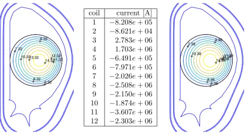
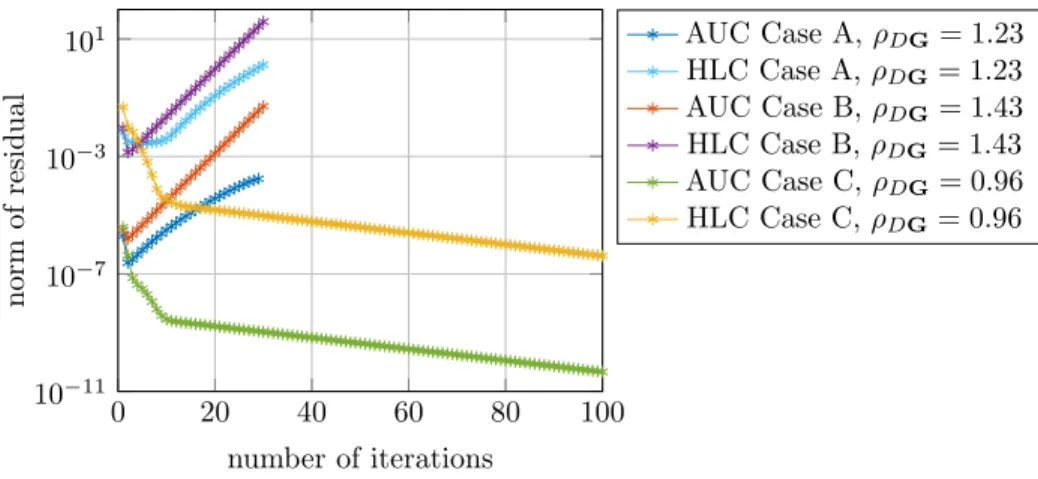
Additionally to the equilibrium from the previous section (see Figure 5) we consider two equilibria with circular boundary that have a contact point with the left, respectively the right side of the limiter (see Figures 8 and 9). We used an inverse problem formulation with prescribed desired boundary [19, Section 2.2] to identify currents (see the tables in Figures 8 and 9). Again as in the case A, the Newton methods for AUC and HLC converge also for the case B and C in less than 10 iterations, where here we took for simplicity random perturbations of the numerical solution as initial guess. As we do not focus on global convergence this is reasonable. But it is important to understand the behavior of fixed point iterations for such random perturbation. In figure 10 we present the convergence history of fixed-point iterations for AUC and HLC for the three di↵erent test cases. We observe that the fixed point iterations for AUC and HLC do not converge for the test cases A and B and that the convergence for the test case C is extremely slow. Fixed point iterations can fail both for elongated as well as circular equilibria. To show that this observation it not related to our choice of perturbation, we recall that the convergence of fixed point iterations is determined by the spectral radius ⇢DG(U) (maximum
among the absolute values of the eigenvalues of DG(U)), where DG(U) is the Jacobian of the function G(U) that defines the fixed point iteration:
Uk+1= G(Uk) .
We have convergence of the sequence (Uk) to the fixed point U⇤, with U⇤ =
G(U⇤) if the spectral radius ⇢
DG is smaller than one. Since we are able to
compute the derivatives required for Newton-type iterations, we are also able to compute the derivatives of the functions G that define the fixed point iterations for AUC and HLC. The power iteration method in turn allows to compute the spectral radius. Computing the spectral radius, the convergence indicator, for the example from Figure 10, we find that indeed its value is larger than one in the cases where we observe no convergence (see legend of Figure 10 for the numbers). Moreover, in case C where we see convergence, the spectral radius is smaller than one. Nevertheless, its values are still fairly large, which explains the extremely slow speed of convergence.
Ultimately, we would like to stress that the size of the spectral radius, hence the success of fixed point iterations is not related to the discretization parameter. In table 3 we show the values of the spectral radius for AUC and HLC for the three di↵erent test cases for sequence of finer and finer meshes. Newton method
14.32 13.32 12.3211.32 10.32 9.32 8.32 7.32 6.32
coil current [A] 1 8.208e + 05 2 8.621e + 04 3 2.783e + 06 4 1.703e + 06 5 6.491e + 05 6 7.971e + 05 7 2.026e + 06 8 2.508e + 06 9 2.150e + 06 10 1.874e + 06 11 3.607e + 06 12 2.303e + 06 14.3813.38 12.3811.38 10.38 9.38 8.38 7.38 6.38
Figure 8: Case B: The currents in the coils (center) and contour plots of numerical solutions using AUC (left) and HLC (right).
Case A Case B Case C
h vol. [m3] ⇢
DG vol. [m3] ⇢DG vol. [m3] ⇢DG
AUC HLC AUC HLC AUC HLC
0.22 845.13 1.29 1.25 490.88 1.47 1.47 489.84 0.95 0.95 0.16 834.72 1.24 1.24 486.81 1.46 1.45 486.34 0.96 0.96 0.11 832.26 1.23 1.23 484.56 1.43 1.43 486.22 0.96 0.96 0.08 831.04 1.25 1.24 484.88 1.45 1.45 485.75 0.96 0.96 0.06 830.24 1.25 1.24 484.62 1.45 1.46 485.41 0.96 0.96 0.04 830.52 1.24 1.24 484.38 1.45 1.46 485.07 0.96 0.96
Table 3: The spectral radius on a sequence of refined meshes,
converges to the same equilibrium as indicated by the numbers in the columns with header vol. giving the total plasma volume, but the values of the spectral radius remain almost constant.
6. Conclusion
We presented a systematic discussion of four di↵erent approaches to the ap-proximation of free-boundary equilibrium problems which are consistent with the boundary condition at infinity. All four methods utilize boundary inte-gral equations. HLC, the most common method for such kind of applications, basically uses a boundary integral equation to derive non-local Dirichlet con-ditions on the boundary of the computational domain, while the other three approaches are rather based on non-local Neumann conditions. AUC, intro-duced in [2], requires the computational domain to be a semi-circle, which can
14.8 13.8 12.8 11.8 10.8 9.7 8.7 7.7 6.7
coil current [A] 1 6.705e + 05 2 1.373e + 04 3 2.133e + 06 4 1.432e + 06 5 3.774e + 05 6 6.172e + 05 7 1.885e + 06 8 2.359e + 06 9 2.124e + 06 10 1.836e + 06 11 3.491e + 06 12 2.040e + 06 14.82 13.8 12.82 11.82 10.82 9.82 8.82 7.82 6.82
Figure 9: Case C: The currents in the coils (center) and contour plots of numerical solutions using AUC (left) and HLC (right).
0 20 40 60 80 100 10 11 10 7 10 3 101 number of iterations n or m of re si d u al AUC Case A, ⇢DG= 1.23 HLC Case A, ⇢DG= 1.23 AUC Case B, ⇢DG= 1.43 HLC Case B, ⇢DG= 1.43 AUC Case C, ⇢DG= 0.96 HLC Case C, ⇢DG= 0.96
Figure 10: Convergence history of fixed point iterations for AUC and HLC for the three di↵erent test cases A, B and C.
lead to a relatively large number of unknowns. The two standard methods JNC and BMC were never used before in free-boundary equilibrium problems.
We showed that HLC su↵ers from non-optimal convergence, compared to AUC and JNC. This problem can be cured, which in turn increases further the computational time. Moreover, our experiments show that it is inevitable to use Newton-type iterations in order to solve the non-linear discrete problems. This second observation that Newton-type method perform better than fixed point iterations is not new. However, knowing that most of today’s equilibrium codes follow the spirit and ideas of von Hagenow and Lackner [18, 29], and employ some sort of HLC combined with fixed point iterations, we want to stress the limits of this method. Augmenting an existing code based on a fixed-point solver with a Newton-type solver is, at first glance, fairly technical. But then a closer look shows that this is only slightly more complicated than the computation of the plasma domain itself and details can be found in the existing literature [19]. The last important result of the present work is the fact that the computation time of AUC is comparable to HLC or JNC even though the number of degrees of freedom is much larger. This observation makes perfectly sense, once you highlight that the boundary integral equations in HLC and JNC lead to dense blocks in the otherwise sparse matrix that needs to be inverted at each Newton iteration.
References
[1] R. Albanese, R. Ambrosino, and M. Mattei. CREATE-NL+: A robust control-oriented free boundary dynamic plasma equilibrium solver. Fusion Engineering and Design, 9697:664 – 667, 2015. Proceedings of the 28th Symposium On Fusion Technology (SOFT-28).
[2] R. Albanese, J. Blum, and O. Barbieri. On the solution of the magnetic flux equation in an infinite domain. In EPS. 8th Europhysics Conference on Computing in Plasma Physics (1986), pages 41–44, 1986.
[3] R. Albanese, J. Blum, and O. De Barbieri. Numerical studies of the Next European Torus via the PROTEUS code. In 12th Conf. on Numerical Simulation of Plasmas, San Francisco, 1987.
[4] A. Bermudez, D. Gomez, M. C. Muniz, and P. Salgado. A FEM/BEM for axisymmetric electromagnetic and thermal modelling of induction furnaces. International Journal for Numerical Methods in Engineering, 71(7):856– 878, 2007.
[5] J. Bielak and R. C. MacCamy. An exterior interface problem in two-dimensional elastodynamics. Quart. Appl. Math., 41(1):143–159, 1983/84. [6] J. Blum. Numerical simulation and optimal control in plasma physics.
[7] J. Blum, C. Boulbe, and B. Faugeras. Real-time plasma equilibrium re-construction in a tokamak. In Journal of Physics: Conference Series. Pro-ceedings of the 6th International Conference on Inverse Problems in Engi-neering: Theory and Practice, volume 135, page 012019. IOP Publishing, 2008.
[8] J. Blum, C. Boulbe, and B. Faugeras. Reconstruction of the equilibrium of the plasma in a tokamak and identification of the current density profile in real time. Journal of Computational Physics, 231(3):960 – 980, 2012. [9] J. Blum, J. Le Foll, and B. Thooris. The self-consistent equilibrium and
di↵usion code SCED. Computer Physics Communications, 24:235 – 254, 1981.
[10] L. Chen. Programming of finite element methods in Matlab, 2011. [11] M. Costabel, V.J. Ervin, and E.P. Stephan. Experimental convergence
rates for various couplings of boundary and finite elements. Mathematical and Computer Modelling, 15(3):93 – 102, 1991.
[12] M. Costabel and E.P. Stephan. Coupling of finite and boundary element methods for an elastoplastic interface problem. SIAM J. Numer. Anal., 27(5):1212–1226, 1990.
[13] F. Cuvelier, C. Japhet, and G. Scarella. An efficient way to assemble finite element matrices in vector languages. BIT, 56(3):833–864, 2016.
[14] J. P. Freidberg. Ideal Magnetohydrodynamics. Plenum US, 1987.
[15] G.N. Gatica and G.C. Hsiao. The uncoupling of boundary integral and finite element methods for nonlinear boundary value problems. J. Math. Anal. Appl., 189(2):442–461, 1995.
[16] J. P. Goedbloed and S. Poedts. Principles of magnetohydrodynamics: with applications to laboratory and astrophysical plasmas. Cambridge university press, 2004.
[17] V. Grandgirard. Mod´elisation de l’´equilibre d’un plasma de tokamak. PhD thesis, Universit´e de Franche-Comt´e, 1999.
[18] K.v. Hagenow and K. Lackner. Computation of axisymmetric MHD equi-libria. In 7th Conf. on Numerical Simulation of Plasmas, New York, page 140, 1975.
[19] H. Heumann, J. Blum, C. Boulbe, B. Faugeras, G. Selig, J.-M. An´e, S. Br´emond, V. Grangirard, P. Hertout, and E. Nardon. Quasi-static free-boundary equilibrium of toroidal plasma with CEDRES++: computational methods and applications. J. Plasma Physics, 2015.
[20] F.L. Hinton and R.D. Hazeltine. Theory of plasma transport in toroidal confinement systems. Rev. Mod. Phys., 48:239–308, Apr 1976.
[21] R. Hiptmair. Coupling of finite elements and boundary elements in elec-tromagnetic scattering. SIAM J. Numer. Anal., 41(3):919–944, 2003. [22] George C. Hsiao and Shangyou Zhang. Optimal order multigrid methods
for solving exterior boundary value problems. SIAM J. Numer. Anal., 31(3):680–694, 1994.
[23] M. Itagaki and T. Fukunaga. Boundary element modelling to solve the Grad-Shafranov equation as an axisymmetric problem. Engineering Anal-ysis with Boundary Elements, 30(9):746 – 757, 2006.
[24] M. Itagaki, J. Kamisawada, and S. Oikawa. Boundary-only integral equa-tion approach based on polynomial expansion of plasma current profile to solve the Grad-Shafranov equation. Nuclear Fusion, 44(3):427, 2004. [25] J.D. Jackson. Classical electrodynamics. Wiley, 1975.
[26] S.C. Jardin. Computational methods in plasma physics. Boca Raton, FL : CRC Press/Taylor & Francis, 2010.
[27] C. Johnson and J. C. Nedelec. On the coupling of boundary integral and finite element methods. Mathematics of Computation, 35(152):pp. 1063– 1079, 1980.
[28] J. Koko. Vectorized Matlab codes for linear two-dimensional elasticity. Sci. Program., 15(3):157–172, August 2007.
[29] K. Lackner. Computation of ideal MHD equilibria. Computer Physics Communications, 12(1):33 – 44, 1976.
[30] L.L. Lao, J.R. Ferron, R.J. Geoebner, W. Howl, H.E. St. John, E.J. Strait, and T.S. Taylor. Equilibrium analysis of current profiles in Tokamaks. Nuclear Fusion, 30(6):1035, 1990.
[31] P.J. Mc Carthy, P. Martin, and W. Schneider. The CLISTE Interpretive Equilibrium Code. Technical Report IPP Report 5/85, Max-Planck-Institut fur Plasmaphysik, 1999.
[32] J.-M. Moret, B.P. Duval, H.B. Le, S. Coda, F. Felici, and H. Reimerdes. Tokamak equilibrium reconstruction code LIUQE and its real time imple-mentation. Fusion Engineering and Design, 91(0):1–15, 2015.
[33] Stefan A. Sauter and Christoph Schwab. Boundary element methods, vol-ume 39 of Springer Series in Computational Mathematics. Springer-Verlag, Berlin, 2011. Translated and expanded from the 2004 German original. [34] F.-J. Sayas. The validity of Johnson-Nedelec BEM-FEM coupling on
[35] O. Steinbach. Numerical approximation methods for elliptic boundary value problems. Springer, New York, 2008. Finite and boundary elements, Trans-lated from the 2003 German original.
[36] E.P. Stephan. Coupling of finite elements and boundary elements for some nonlinear interface problems. Comput. Methods Appl. Mech. Engrg., 101(1-3):61–72, 1992.
[37] T. Takeda and S. Tokuda. Computation of MHD equilibrium of tokamak plasma. J. Comput. Phys., 93(1):1–107, 1991.
[38] J. Wesson. Tokamaks. The International Series of Monographs in Physics. Oxford University Press, 2004.
[39] K. Zhao, M.N. Vouvakis, and J.-F. Lee. Solving electromagnetic problems using a novel symmetric fem-bem approach. Magnetics, IEEE Transactions on, 42(4):583–586, April 2006.
[40] O.C Zienkiewicz, D.W. Kelly, and P. Bettess. Marriage `a la mode - the best of both worlds (finite elements and boundary integrals). In R. Glowin-ski, E.Y. Rodin, and O.C. Zienkiewicz, editors, Energy Methods in Finite Element Analysis, pages 81–107. Wiley, Chichester, UK, 1979.
RESEARCH CENTRE
SOPHIA ANTIPOLIS – MÉDITERRANÉE
2004 route des Lucioles - BP 93 06902 Sophia Antipolis Cedex
Publisher Inria
Domaine de Voluceau - Rocquencourt BP 105 - 78153 Le Chesnay Cedex inria.fr