HAL Id: hal-00945970
https://hal.archives-ouvertes.fr/hal-00945970
Submitted on 31 Mar 2020HAL is a multi-disciplinary open access archive for the deposit and dissemination of sci-entific research documents, whether they are pub-lished or not. The documents may come from teaching and research institutions in France or abroad, or from public or private research centers.
L’archive ouverte pluridisciplinaire HAL, est destinée au dépôt et à la diffusion de documents scientifiques de niveau recherche, publiés ou non, émanant des établissements d’enseignement et de recherche français ou étrangers, des laboratoires publics ou privés.
A beam to 3D model switch in transient dynamic
analysis
Mikhael Tannous, David Dureisseix, Patrice Cartraud, Mohamed Torkhani
To cite this version:
Mikhael Tannous, David Dureisseix, Patrice Cartraud, Mohamed Torkhani. A beam to 3D model switch in transient dynamic analysis. European Congress on Computational Methods in Applied Sciences and Engineering, 2012, Vienna, Austria. �hal-00945970�
A beam to 3D model switch for transient dynamic analysis
Conference Paper · January 2012
CITATIONS 6
READS 126
4 authors, including:
Some of the authors of this publication are also working on these related projects:
wood science for conservation of cultural heritageView project
Ship Ultimate Strength under WhippingView project Mikhael Tannous
12 PUBLICATIONS 85 CITATIONS SEE PROFILE
Patrice Cartraud
Ecole Centrale de Nantes
110 PUBLICATIONS 1,837 CITATIONS SEE PROFILE
David Dureisseix
Institut National des Sciences Appliquées de Lyon
193 PUBLICATIONS 1,278 CITATIONS SEE PROFILE
European Congress on Computational Methods in Applied Sciences and Engineering (ECCOMAS 2012) J. Eberhardsteiner et.al. (eds.) Vienna, Austria, September 10-14, 2012
A BEAM TO 3D MODEL SWITCH IN TRANSIENT DYNAMIC
ANALYSIS
Mikhael Tannous1, Patrice Cartraud1, David Dureisseix2, and Mohamed Torkhani3
1G´eM, Ecole Centrale de Nantes
address
e-mail:{mikhael.tannous,patrice.cartraud}@ec-nantes.fr
2Lamcos, INSA de Lyon
address
e-mail: [email protected] 3EDF, R&D, Clamart
address
e-mail: [email protected]
Keywords: dynamics, finite element, switch
Abstract. Many industrial problems involving slender structures in transient dynamics require a3D model for a better understanding of local or non linear effects that occur along a small
period of time, whereas a simplified beam model can be sufficient for simulating the linear phenomena occurring for a long period of time.
This paper proposes a method which enables to switch from a beam to a 3D model during a
transient dynamic analysis solved with a time integration technique. Thus, this method allows to reduce the computational cost while preserving a good accuracy.
Starting with the beam model, at switch momentts, a3D solution is constructed as the sum of
a cross-section rigid body displacement corresponding to the classical Timoshenko kinematical
assumption and a3D correction which accounts for cross-section deformation. This correction
is obtained from the solution of a static problem and may be computed on three consecutive time steps (the switch instant, the previous and the following steps) thus allowing to make a velocity and acceleration corrections based on the three static computations. The dynamic simulation
is initialized atts by the displacements, velocities and accelerations being computed.
The method is validated through comparisons with a reference solution corresponding to the
1 INTRODUCTION
Many industrial problems in transient dynamics, such as the simulation of turbine accidents, require a3D model for a better understanding of non linear local effects such as rubbing, that occur along a small period of time. However, a 3D model for the entire rotor and the entire stator used during the whole simulation will result in an unaffordable computational time. We therefore, present a method that can dramatically reduce the computational time, for problems where the3D non linearities are restricted in space and time.
For non linear phenomena that are restricted in time, one can use a time integration scheme switching technique. An implicit/explicit or explicit/implicit switching algorithm may reduce the computational costs such as described in [14, 15, 13, 16]. However, since in turbine ac-cidents simulations, the non linearities are also restricted in space, time integration scheme switching will not lead to optimal computational cost.
Other approaches in the literature deal with reducing the computational cost of 2D or 3D models by using different mesh densities or models. Adaptive meshing techniques can take the form of a local refinement of a3D model, such as in [10, 11, 17] or a beam to 3D refinement as done in [9] for the simulation of a bridge deformation. The beam and the local3D refinement are connected by mathematical constraints. Domain decomposition techniques are also well known in this field to reduce computational cost while being accurate and examples can be found in [8], [7], [3, 12] and others. For this same purpose FETI domain decomposition methods were developed and used in [5, 2, 1, 6, 4].
These CPU time reducing techniques are very interesting. However, since non linearities are restricted in space and time, the optimal computational cost can not be achieved unless no 3D model at all is present during the linear stage, which means the use of a beam model. The turbine rotor with rubbing was modelled by a beam in [19] and [20]. However, the beam model is not adapted to treat accurately local rotor stator interactions and a3D model is needed for a better understanding of local non linear effects. Therefore, a numerical strategy which enables to use a 3D or beam model at different stages of the transient analysis allows to reduce the computational cost while preserving a good accuracy is proposed here, as illustrated in Fig. 1. In fact, the simulation starts att = t0 with a beam model for a linear simulation, and switches
att = ts1 to a3D model when a non linear phenomenon is to take place. The simulation is to
be switched back att = ts2to the beam model for of the rest of the simulation that ends attf, if
no more non linear phenomena are present.
Beam model Beam model
Beam to 3D switch 3D to beam switch
ts1 ts2 tf
t0
3D model
linear simulation linear simulation
non linear simulation Figure 1: Beam to3D switch
Mikhael Tannous, Patrice Cartraud, David Dureisseix and Mohamed Torkhani
beam to3D model switch, the 3D to beam model switch is not addressed here.
2 MATHEMATICAL BASICS OF THE SWITCH
A beam model simulation that started att = 0 is to be switched for a 3D model simulation at t = ts. Starting with the 3D model at t = ts requires the collection of the beam model
solution at ts and transforming this solution to have a suitable3D model initialization at the
same moment.
The fundamental dynamic equation of a beam att = tscan be written:
MbU¨b+ CbU˙b+ KbUb = fb (1) where, Mb , Cb, and Kb are respectively the mass, damping and stiffness matrices of the beam
model.
The3D model at t = tscan be described by:
M3DU¨3D+ C3DU˙3D+ K3DU3D = f3D (2) where, M3D , C3D, and K3D are respectively the mass, damping and stiffness matrices of
the3D model.
Suppose that we start with the beam model, at switch moment (t = ts), we have to construct
the 3D solution U3D from the beam solution. This is performed first by decomposing the
3D displacement into a cross-section rigid body displacement corresponding to the classical Timoshenko kinematical assumption PUb, and a3D correction U3Dcwhich accounts for
cross-section deformation:
U3D = U3Dc+ PUb (3)
We therefore need to generate PUb and to compute U3Dcin order to construct the3D model
displacement atts.
2.1 Generating PUb
PUb is obtained through a projector matrix P which transforms the beam displacement vector into a3D rigid body displacement. However, it is not easy to build P because it depends on the relationship between the beam mesh and the 3D mesh, which may change from one cross-section to another. Instead, we will generate PUb as a whole.
LetNij a node that belongs to the ithcross-section of the3D model, PUijb is the
displace-ment ofNij computed for a cross-section rigid body displacement. The cross-section to which
belongsNij hasGi for its gravity center. Theith beam node has a displacement Uib and a
rota-tional displacementθi
b. With the finite element software used, such as Code Aster or Abaqus,
we write a python loop that manages to compute PUijb = [PUijbx, PUijby, PUijbz] for each node Nij as follows: PUij b = U i b+ NiGi∧ θib (4) 2.2 Computing U3Dc
Due to the decomposition of the 3D displacement according to Eq. (3), the3D model initial-isation will be performed through the3D correction U3Dc. Thus, inserting Eq. (3) in Eq. (2) at
(t = ts) gives:
M3D(U¨
3Dc+ ¨PUb) + C3D( ˙U3Dc+ ˙PUb) + K3D(U3Dc+ PUb) = f3D (5)
Since we have one equation with three unknowns, then making the following assumptions:
˙
U3Dc = 0 ¨
U3Dc = 0 (6)
will result in a displacement correction U3Dcthat corresponds to a static computation for the
3D model, at t = ts, and that is the solution of the following equation:
K3DU3Dc= f3D− M3DPU¨ b− C3DPU˙ b− K3DPUb (7) The computations of P ˙Uband P ¨Ub can be done in the same way as PUb by substituting in Eq. (4) Ubby ˙Ub or ¨Ub.
Then one can switch to the3D model which is initialized at t = tsby:
U3D = U3Dc+ PUb ˙
U3D = P ˙Ub ¨
U3D = P ¨Ub (8)
With this choice, only the displacements are different from the cross-section rigid-body dis-placement assumption at the switch instant. However, the initialization of the accelerations and velocities are a critical issue in many integration schemes such as several integration schemes of the Newmark integration scheme family, or the central difference scheme. Since no correc-tion has been developed for the velocities or acceleracorrec-tions, it means that they will be different with the3D reference ones. In most cases of study shown later in this paper, this difference is around 5% on velocities and accelerations, which seems to be quite small. However, this in-duces a transient phenomenon in which high frequency oscillations occur, which are an artefact of this initialization. These high frequency oscillations may lead the solution to diverge. In order to vanish these oscillations, one can insert a numerical damping or make velocities and accelerations correction as detailed in Section 3.
3 INITIALIZING THE 3D SOLUTION
3.1 Numerical damping (HHT integration technique)
A numerical damping in the integration scheme can filter these high frequency oscillations without any other influence on the solution. The HHT integration scheme has been used to filter the numerical oscillations. This numerical damping needs to be maintained on the several time steps following the switch in order the high frequency oscillations vanish, as shown in the following results. However, a more attractive method does exist and can reduce considerably the high frequency oscillations that appear after switching and is detailed in Section 3.2.
3.2 A triple static switch procedure
As Eq. (8) shows, the high frequency oscillations are generated by a poor initialization of the velocities and accelerations, since these later are generated from the beam solution and are
Mikhael Tannous, Patrice Cartraud, David Dureisseix and Mohamed Torkhani
not completely adapted to the 3D model. The hypothesis taken in Eq. (6) is too strong and generates high frequency oscillations. However, assuming that the displacement initialization is adapted to the3D model, then a strategy enabling a better initialization of the velocities and accelerations based on the displacement correction can be built with the integration scheme and thus eliminates the high frequency transient phenomenon that occurs after switching.
We therefore first check the displacement correction on a static problem to prove its efficiency and then, according to the integration scheme being used, construct velocity and acceleration initializations.
3.2.1 The switch for static problems
The switch for a static problem may be seen as a particular case of the dynamic one. It is investigated here to test if the 3D displacements after switching are close to a reference 3D static solution. The beam fundamental equation for a static problem is:
KUb = fb (9)
The3D fundamental equation is:
K3DU3D = f3D (10)
The 3D displacement can be divided as explained earlier in Eq. (3), and that will lead to define U3Dcas the solution of:
K3DU3Dc = f3D− K3DPUp (11) This static correction U3Dc summed with PUb is compared to a reference solution for the
same3D model mesh, computed by solving Eq. (10). This has been performed on several mesh types, cross-sections shapes and boundary conditions, and the difference between the computed displacements and the reference solution has been found to be negligible, indicating that the displacements are well corrected by this switch method.
3.2.2 Basics of the triple static switch procedure
Since a static switch provides an accurate correction of the 3D displacements, a correction of the velocities and accelerations can be built using three static switch procedures at three consecutive time steps. The velocities and accelerations andt = tswill be computed from the
displacement values at this instant and at one step before this instant and one step after. From these values, velocities and accelerations will be obtained through the same expressions as those used in the time integration technique chosen for solving the problem. This procedure is based on the knowledge of the time integration technique used to solve for the dynamic equation of motion.
The integration technique mostly used in Code Aster is implicit, and especially the New-mark integration scheme. In [18], we find a detailed description of the NewNew-mark integration technique. The velocity is computed by:
˙
Un+1 = ˙Un+ (1 − γ)∆T ¨Un+ γ∆T Un+1 (12)
where U, ˙U, and ¨U are respectively the displacements, velocities and accelerations. ∆T denotes the step time. n is the current step and n + 1 is the following one. One has also β and γ being the Newmark parameters. The displacements are computed by:
Un+1 = Un+ ∆T ˙Un+ ∆T2(1
2 − β) ¨Un+ ∆T
2
β ¨Un+1 (13) The Newmark integration scheme is consistent because it can be proved that one has:
lim ∆T →0 ˙ Un+1− ˙Un ∆T = ¨Un (14) and lim ∆T →0 Un+1− Un ∆T = ˙Un (15)
Thus we define the acceleration att = tsby:
¨ U = ˙ Un+1− ˙Un ∆T = Un+1−Un ∆T − Un−Un−1 ∆T ∆T = Un+1− 2Un+ Un−1 ∆T2 (16)
and initialize the3D model by the following velocities and accelerations: ˙
U3D = [PUb+ U3Dc]ts+1 − [PUb+ U3Dc]ts−1
2∆T (17)
¨
U3D = [PUb+ U3Dc]ts+1− 2[PUb+ U3Dc]ts + [PUb+ U3Dc]ts−1
∆T2 . (18)
This method is as accurate as the time step is small, since it is demonstrated that for suffi-ciently small time steps, it is consistent with the Newmark integration scheme in use. Never-theless, the time step in use with the Newmark family is always finite, and thus the transient phenomenon will still be observed on the first4 to 5 time steps that follows the switch. How-ever, the high frequency oscillations present a very low amplitude, and vanish in the scope of the following4 to 5 time steps that follows the switch. We therefore can propose this initialization of the3D model as a proper beam to 3D model switching technique.
4 APPLICATION EXAMPLES
In this section, we present a simple numerical example that illustrates the efficiency of the beam to3D model switch for dynamic cases. In fact, the method has been validated on more complex cases, for different type of cross-section shapes, loadings and boundary conditions. In the case considered here, the beam model is a Timoshenko beam model, with a rectangular cross-section, having the following dimensions: width 0.012 m, height 0.01 m and a clamped a length of 0.1m. The beam is made with a steel material with densityρ = 7800 kg/m, Young modulusE = 2.1 × 10¹¹
N/m2
and Poisson coefficient0.3. One side of the beam is fixed, the other one is subjected to a concentrated dynamic load equal to f(t) = 100 × t × e−1.1t
at its surface center. Fig. 2 illustrates the 3D model. The 3D model is quadratically meshed with approximately one thousands nodes. The switch instant ists = 1.5 s, at which the beam
sim-ulation is switched to the3D model, with the same boundary conditions and loading. The 3D solution after switching is compared to a reference solution, which is a3D solution obtained on
Mikhael Tannous, Patrice Cartraud, David Dureisseix and Mohamed Torkhani
the same3D model for a simulation that starts at t = 0 and lasts three seconds.
This work is done twice. The switch from the beam model to the 3D model is performed
P
P
f(t)
Figure 2: The3D model under study
first using the approach described in Section 3.1 (static correction only) and second with the initialization built from the3D displacements computed at three different time steps (see Sec-tion 3.2.2).
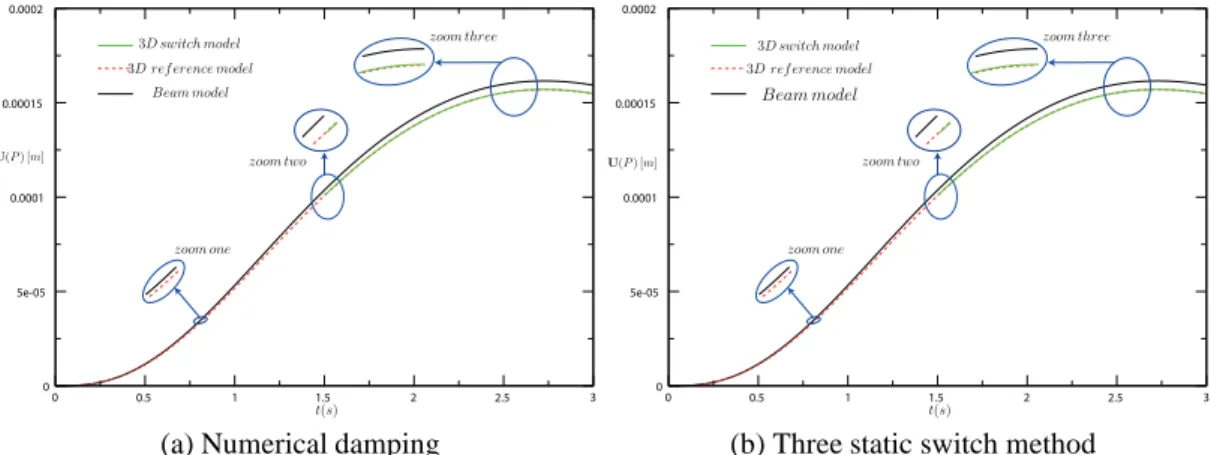
We compare the displacements, velocities and accelerations of nodeP where the load is exerted and that belongs to the3D model as shown on Fig. 2, and the corresponding point that belongs to the beam model.
Fig. 3 shows the displacement results. First we can see a certain difference between the beam solution and the3D reference solution. This difference is very small, but still remarkable if we make a zoom. Immediately after switching, the3D solution turns out to be very accurate and is very close to the reference one. Both methods exhibit practically the same precision regarding the displacements.
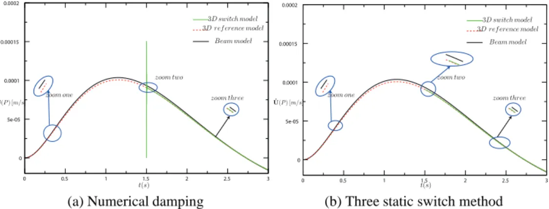
However, as shown on Fig. 4, which represents a velocity comparison, or Fig. 5 which
rep-0 0.5 1 1.5 2 2.5 3 0 5e-05 0.0001 0.00015 0.0002 Beam model 3D switch model 3D ref erence model
zoom one zoom two
zoom three
t(s)
U(P ) [m]
(a) Numerical damping
0 0.5 1 1.5 2 2.5 3 0 5e-05 0.0001 0.00015 0.0002 Beam model 3D switch model 3D ref erence model
zoom one zoom two
zoom three
t(s)
U(P ) [m]
(b) Three static switch method Figure 3: Beam to3D model switch: displacement analysis
resents an acceleration comparison, immediately after switching, high frequency oscillations with large amplitude occur in the case where there is only the static correction. For a HHT integration scheme withα = 0.25, in our case 35 time steps (0.02625 s) were sufficient for the 3D solution to converge to the reference one.
If a tripe static switch procedure is performed, the velocities do not present any oscillations; however, very small oscillations occur on the accelerations and vanish shortly after switching. The results show that both methods work, but the triple static switch procedure appears to be more accurate.
0 0.5 1 1.5 2 2.5 3 0 5e-05 0.0001 0.00015 0.0002 Beam model 3D switch model 3D ref erence model
zoom one zoom two zoom three t(s) ˙ U(P ) [m/s]
(a) Numerical damping
0 0.5 1 1.5 2 2.5 3 0 5e-05 0.0001 0.00015 0.0002 Beam model 3D switch model 3D ref erence model
zoom one zoom two zoom three t(s) ˙ U(P ) [m/s]
(b) Three static switch method Figure 4: Beam to3D model switch: velocity analysis
0.5 1 1.5 2 2.5 3 -5e-05 0 5e-05 0.0001 0.00015 Beam model 3D switch model 3D ref erence model zoom one zoom two zoom three t(s) ¨ U(P ) [m/s2]
(a) Numerical damping
0 0.5 1 1.5 2 2.5 -5e-05 0 5e-05 0.0001 0.00015 Beam model 3D switch model 3D ref erence model
zoom one
zoom two zoom three
t(s)
¨ U(P ) [m/s2
]
(b) Three static switch method Figure 5: Beam to3D model switch: acceleration analysis
5 CONCLUSIONS
We have proposed a numerical method that enables to switch from a beam to a 3D model when a3D description is required only on a small part of space and time domains. This tech-nique enables to save computational time, with a good accuracy. The authors are currently developing this method in the case of rotating machine for application to the slowing down of unbalanced turbine rotors with local interactions and frictions.
ACKNOWLEDGMENTS
The authors thank the French National Research Agency (ANR) in the frame of its Techno-logical Research COSINUS program. (IRINA, project ANR 09 COSI 008 01 IRINA)
REFERENCES
[1] P. Avery and C. Farhat. The feti family of domain decomposition methods for inequality-constrained quadratic programming: Application to contact problems with conforming and nonconforming interfaces. Computer Methods in Applied Mechanics and
Engineer-ing, 198:1673–1683, 2009.
[2] P. Avery, G. Rebel, M. Lesoinne, and C. Farhat. A numerically scalable dual-primal substructuring method for the solution of contact problems part i: the frictionless case.
Mikhael Tannous, Patrice Cartraud, David Dureisseix and Mohamed Torkhani
Computer Methods in Applied Mechanics and Engineering, 193:2403–2426, 2004.
[3] L. Champaney. A domain decomposition method for studying the effects of missing fas-teners on the behavior of structural assemblies with contact and friction. Computer
Meth-ods in Applied Mechanical Engineering, 208:121–129, 2012.
[4] C. Farhat and J. Li. An iterative domain decomposition method for the solution of a class of indefinite problems in computational structural dynamics. Applied Numerical
Mathematics, 54:150–166, 2005.
[5] C. Farhat, J. Mandel, and F.-X. Roux. Optimal convergence properties of the feti do-main decomposition method. Computer method in Applied Mechanics and Engineering, 115:365–385, 1994.
[6] C. Farhat, K. Pierson, and M. Lesoinne. The second generation feti methods and their application to the parallel solution of large-scale linear and geometrically non-linear struc-tural analysis problems. Computer Methods in Applied Mechanics and Engineering,
184:333–374, 2000.
[7] V. Faucher and A. Combescure. A time and space mortar method for coupling linear modal subdomains and non-linear subdomains in explicit structural dynamics. Computer
Methods in Applied Mechanics and Engineering, 192:509–533, 2003.
[8] P. Gosselet and C. Rey. Non-overlapping domain decomposition methods in structural mechanics. Archives of Computational Methods in Engineering, 11:1–50, 2005.
[9] P. Kettil and N.-E. Wiberg. Application of 3d solid modeling and simulation programs to a bridge structure. Engineering with Computers, 18:160–169, 2002.
[10] M. Kimura, H. Momura, M. Mimura, H. Miyoshi, T. Takaishi, and D. Ueyama. Adaptive mesh finite element method for pattern dynamics in reaction-diffusion systems. In
Pro-ceedings of the Czech-Japanese Seminar in Applied Mathematics, Kuju Training Center, Oita, Japan, 2005.
[11] X. Li and N.-E. Wiberg. Implementation and adaptivity of a space-time finite element method for structural dynamics. Computer Methods in Applied Mechanics and
Engineer-ing, 156:211–229, 1998.
[12] O. Lloberas-Valls, D.J. Rixen, A. Simone, and L.J. Sluys. Domain decomposition tech-niques for the efficient modeling of brittle heterogeneous materials. Computer Methods in
Applied Mechanical Engineering, 200:1577–1590, 2011.
[13] N. Mahjoubi, A. Gravouil, and A. Combescure. Coupling subdomains with heterogeneous and incompatible time steps. Computational Mechanics, 44:825–843, 2009.
[14] L. Noels, L. Stainier, and J.-P. Ponthot. Combined implicit/explicit algorithms for crash-worthiness analysis. International Journal of Impact Engineering, 30:1161–1177, 2004. [15] L. Noels, L. Stainier, and J.-P. Ponthot. Combined implicit/explicit time-integration
algo-rithms for the numerical simulation of sheet metal forming. Journal of Computational and
Applied Mathematics, 168:331–339, 2004.
[16] K. C. Park, S. J. Lim, and H. Huh. A method for computation of discontinuous wave propagation in heterogeneous solids: basic algorithm description and application to one-dimensional problems. international Journal for Numerical Methods in Engineering, 4285, 2012.
[17] A. Plaza, M. Padron, and G. Carey. A 3d refinement/derefinement algorithm for solving evolution problems. Applied Numerical Mathematics, 32:401–418, 2000.
[18] D. Rixen. Multi-body dynamics: time integration, 2002.
[19] S. Roques. Modlisation du comportement dynamique couple rotor-stator d’une turbine en
situation accidentelle. PhD thesis, Ecole Centrale de Nantes, 2007.
[20] S. Roques, M. Legrand, P. Cartraud, C. Stoisser, and C. Pierre. Modeling of a rotor speed transient response with a radial rubbing. Journal of Sound and Vibration, 329:527–546, 2009.