Asymptotic Numerical Method applied to stability and bifurcation analysis of a boiling flow at low pressure in a pipe

(1)

HAL Id: cea-02339077

https://hal-cea.archives-ouvertes.fr/cea-02339077

Submitted on 13 Dec 2019

HAL is a multi-disciplinary open access archive for the deposit and dissemination of sci-entific research documents, whether they are pub-lished or not. The documents may come from teaching and research institutions in France or abroad, or from public or private research centers.

L’archive ouverte pluridisciplinaire HAL, est destinée au dépôt et à la diffusion de documents scientifiques de niveau recherche, publiés ou non, émanant des établissements d’enseignement et de recherche français ou étrangers, des laboratoires publics ou privés.

bifurcation analysis of a boiling flow at low pressure in a

pipe

E. Bissen, M. Médale, N. Alpy

To cite this version:

E. Bissen, M. Médale, N. Alpy. Asymptotic Numerical Method applied to stability and bifurcation analysis of a boiling flow at low pressure in a pipe. 12th International Topical Meeting on Reactor Thermal-Hydraulics, Operation, and Safety (NUTHOS-12), Oct 2018, Qingdao, China. �cea-02339077�

(2)

Abstract No: 30 Paper No.:

Asymptotic Numerical Method applied to stability and bifurcation analysis of a boiling

flow at low pressure in a pipe

Edouard Bissen, Marc Medale

Aix-Marseille University, IUSTI, CNRS UMR 7343, F-13453 Marseille, France

edouard.bissen@etu.univ-amu.fr, marc.medale@univ-amu.fr Nicolas Alpy

CEA, DEN, DER, SESI, LEMS, F-13108 Saint Paul Lez Durance,

France

nicolas.alpy@cea.fr

ABSTRACT

In the framework of the R&D on GEN IV Sodium-cooled Fast Reactors (SFRs) at the CEA, a hypothetical Unprotected Loss of Flow (ULOF) is investigated and could lead to sodium boiling if one assumes the non-activation of passive complementary safety devices. As a qualification basis, the CEA is currently developing and coupling reference codes at different scales. Supposing a complete integrity of hydraulic channels geometry, reactor case studies have shown the possibility of a periodic boiling regime: the density wave mechanism, which is believed to be enhanced by low void worth core design distinctive of a GEN IV SFR, is interestingly characterized by pins claddings cooling possibility at sodium saturation temperature (instead of dry-out). In that scientific framework, this paper presents the ongoing development of an innovative semi-analytical methodology to perform stability and bifurcation analyses of boiling flows. While equations for a 1D multiphase model based on a drift model are classically used, the Asymptotic Numerical Method (ANM) is implemented to solve steady-state equations whose non linearities drive the observed dynamic phenomena. Inline, elements of the Theory of Dynamical Systems are first recalled, such as the Hopf bifurcation linked to the appearance of a periodic solution and its stability, to provide the necessary mathematical background. The added-value for this specific study of the ANM over a zero-order continuation method is illustrated on a test case. Some simulation results are then reported to investigate flow phenomenology that was addressed along boiling stability experiments led by Saha in 1970's. On one hand, the runs show our model’s numerical ability to efficiently handle a non-linear set of equations while imposing a numerically stringent pressure difference for flow boundary conditions; on the other hand, no qualitative evidence of unstability onset has been observed while such a phenomenon is the central point of Saha experimental work. Even if only eigenvalues analysis, to be next carried out, could assert a miss of the model, this point could reveal some limitations regarding the set of closure laws or geometrical description that is up to now considered in our model. To support this statement, some additional simulation results on an academic case are given which exhibit how a non linearity of the model, not engaged in the Saha experimental conditions, could lead to an oscillating response in the bifurcation diagram.

KEYWORDS

Thermal-hydraulics, stability of boiling flows, semi-analytical methods, continuation methods.

1. INTRODUCTION

The fourth generation of nuclear reactors is focusing on enhanced safety requirements and closing the fuel cycle. There has therefore been a lot of research on Sodium-cooled Fast Reactors (SFRs) at the CEA [1]. As for the safety, hypothetical scenarios are extensively studied such as an Unprotected Loss

(3)

of Flow (ULOF), assuming the non-actuation of complementary passive safety devices, which can lead to sodium boiling.

Sodium boiling has been studied in the 1980's in France [2] and abroad [3-4] in the geometry typical of SUPERPHENIX (homogeneous core). A static phenomenology was observed and the possibility for a stabilized boiling, avoiding dry-out, was shown thanks to a Ledinegg static stability criterion.

The GEN IV SFR (CFV, French acronym for Low Sodium Void Effect) core characteristics are very different from the previous generation, with a heterogeneous composition and a sodium plenum on top of the fuel bundle. At the CEA, reference codes such as CATHARE for thermal-hydraulics and APOLLO for neutronics have been adapted to sodium and especially the set of closure laws validated and some revised to the GEN IV geometry using experiments such as GR19 [5] and more recently SENSAS [6]. The results illustrated in Fig. 1 show a dynamical phenomenology, with strong oscillations in void fraction or mass flow rate for example. Moreover, some simulations tend to a scenario where these oscillations remain stable, which could enhance safety by keeping the temperature at the saturation level hence avoiding dry-out similarly to the stabilized boiling in the 1980's.

Fig. 1 : Illustration of a dynamic boiling behaviour computed with CATHARE [7].

Elsewhere, dynamic boiling phenomenology and its stability has long been a topic of interest for the Boiling Water Reactors (BWRs). Many experiments have been led as early as in the 1950's to gain a better understanding of the phenomenology and deduce more accurate closure laws, such as two-phase wall friction for example [8]. These experiments were then used as basis for analytical models, like the drift model first developed by Zuber and Findlay [9], then further improved by Saha [10] after his own experiments on oscillations stability, Ishii [11] and more recently Hibiki [11-12]. Such models, specific to the study of boiling dynamic phenomenology, allowed the development of semi-analytical stability analysis methods. The stability criteria derived from these methods were drawn into stability maps depending on reactors' operating parameters as illustrated in Fig. 2 [14]. Further on, the different types of observed oscillations have been classified methodically [15-16]. Thermal-hydraulic drift models have also been coupled to thermomechanics and neutronic models to improve predictions [17].

(4)

Fig. 2 : Illustration of a stability map in the Npch-Nsub space [14].

As detailed in [18], the purpose of the present work is to take advantage of semi-analytical methodologies to deal with the strong non-linear phenomena involved in the related governing equations. This approach should allow to link the physical limit cycle appearing with oscillations such as density waves to a mathematical phenomenon called the Hopf bifurcation, which indicates in the bifurcation diagram the appearance of a periodic solution. Moreover, the study of the characteristics of a Hopf bifurcation gives the stability of the periodic solution. Further on, the occurrence of such phenomena is to be linked to the characteristics of the CFV core. Our approach is based on the Asymptotic Numerical Method (ANM), a high-order predictor-corrector continuation algorithm worked on expertly at the Aix-Marseille University. It enables us to find all solutions of a strongly non-linear problem and especially all the points of interest, such as bifurcation points, where a linear stability anlaysis is particularly relevant. In this paper we illustrate our methodology and its added-value as well as first experimental comparison results based on the data from Saha [19]. Finally we draw some perspectives for the remainder of this PhD work.

2. STATE-OF-THE-ART ON NONLINEAR NUMERICS

2.1. Minimal Background from the Theory of Dynamical Systems

The Theory of Dynamical Systems focuses on non-linear calculations, hence allowing to overcome the usual linearization assumption [20], a crucial point in the case of interest of this paper where strong non-linearities take place.

Let us consider a system of equations, typically Ordinary or Partial Differential Equations (ODEs or PDEs) [21] that read as follows:

(1) where is the unknowns vector, its derivative with respect to time and a parameter. This formulation assumes the time-derivative terms can be written as direct derivative of the unknowns. The stationary solutions of the system, , can be found by solving:

(2) The linear stability of a stationary solution can be defined as follows [22]:

- A solution is called asymptotically stable if its response to small amplitude perturbations tends to zero as time goes to infinity;

(5)

- A solution is called stable if its response to small amplitude perturbations remains small as time goes to infinity;

- A solution is called unstable otherwise.

To compute the linear stability of a steady solution, one introduces small amplitude perturbations, assumed to be exponential in time. This leads to rewriting our system, linearized around the stationary solution, as an eigenvalue problem:

(3) where J is the Jacobian matrix, hence the derivative of all governing equations with respect to all the unknowns, μ is the frequency and w is the spatial amplitude mode of the perturbations.

Therefore, the eigenvalues of the Jacobian matrix of the system give the linear stability, assuming the time derivative terms are written as direct time derivatives of the unknowns like in Eq. (1). If this condition isn’t met, the identity matrix will be replaced by a monodromy matrix [23].

2.2. Continuation Methods and Bifurcation Points

A continuation method is defined as an algorithm able to compute and follow a branch of solutions. A branch of solutions is itself defined as the continuum of solutions of a system parametrised following the lambda parameter defined in Eq. (1). The Implicit Function Theorem stipulates the existence of a branch of stationary solutions if the Jacobian matrix is non-singular for a hyperbolic system.

Using a continuation method ensures to find all the solutions of a system and therefore all the points of interest such as bifurcation points. A bifurcation point is a point where the branch of solutions cannot be extended uniquely. There are three main categories of bifurcation points [22]:

- The turning point, so called because the branch of solutions literally “turns” as illustrated in Fig. 3, is a point where the Jacobian matrix is singular. To find the solution at this point, it has been proposed to add a new equation to the system describing the behaviour of the continuation parameter lambda. This extended system is not singular at the turning point, hence the solution can be computed and the branch of solutions extended uniquely. At a turning point, the stability of the stationary solution changes. Because of the unicity of the branch of solutions at a turning point, many authors consider it not to be a bifurcation point per se.

Fig. 3 : Illustration of a turning point [24].

- The stationary bifurcation is a point where not only the Jacobian is singular, but the extended system as well. This means the branch of solutions cannot be extended uniquely as there are several branches emanating from that point, as illustrated in Fig. 4. A matrix being singular means the dimension of its kernel is higher than one. The decomposition of this kernel gives the number of coexisting branches and their tangent vector. A stability analysis is then necessary for each branch.

(6)

Fig. 4 : Illustration of a stationary bifurcation [24].

- The Hopf bifurcation [25] is different as it is characterized by the appearance of a periodic solution. The Jacobian matrix is not singular at a Hopf bifurcation because the stationary solution is unique and defined. However, its stability changes due to the appearance of the aforementioned periodic solution. A stability analysis is therefore required to determine the stability of both coexisting stationary and periodic solutions. There are two types of Hopf bifurcation depending on the stability evolution scenarios. A Hopf bifurcation is called supercritical is the stationary solution is destabilized by the appearance of a stable periodic solution. It is subcritical otherwise.

Fig. 5 : Illustration of both Hopf bifurcation scenarios [17].

The Asymptotic Numerical Method (ANM) is the continuation method used in this work. This predictor-corrector algorithm is based on an arbitrarily high order Taylor-series decomposition of the unknowns in order to transform the original non-linear set of equations into a set of linear algebraic systems. The mathematical treatment is detailed in [24], so in the remainder we will only introduce the main concepts of the approach. The Taylor series are written with respect to the path parameter, which defines the continuation step along the branch of solutions. This parameter is implicit in the system, which means that the length of each step is adapted to the strength of the non-linearities via the radius of convergence of Taylor series. The stronger the non-linearities, the shorter the continuation step. This

(7)

ensures not to miss any important behaviour, meanwhile allowing optimal step length. On the other hand, the main constraints relateed to the ANM is for every part of the model to be written in a continuous and derivable way. For example, a sudden change of hydraulic diameter of the channel needs to be written using typically a hyperbolic tangent to smoothen it. In the present work the ANM is implemented in the DIAMANLAB software [26] written in MATLAB, that includes the automatic differentiation on top of the continuation algorithm. This allows the derivatives to be computed automatically, no matter the original writing of the equations.

3. METHODOLOGY

3.1. Model Equations

In this section we set our model equations up, which are based on the classical drift formulation [12]. The drift model has been thought specifically for the study of multiphase flows. Its subtle mix of terms describing the mixture behaviour and terms describing the interaction between the two phases via the drift velocity allows it to remain compact in the amount of equations while keeping the ability to study complex phenomena of interest such as density waves [27]. The classic formulation of a 1D drift model includes 4 conservation equations : mixture mass, momentum and energy, and dispersed phase mass [12]. The energy conservation equation is written in its enthalpy form. Let us note that we solve the stationary form of the drift model with the ANM, the time-related terms of the equations being introduced only for the stability analysis.

We decided to modify this classic drift model in stationary form. Let us first expose our equations then detail how they differ from the classic formulation.

We write the mixture mass conservation as:

(4) The stationary form means keeping only the advection term.

The mixture momentum conservation:

(5) We find in the equation an advection, a pressure gradient, a wall friction, a gravity and a drift term. The enthalpy equation:

(6) This equation is composed of an advection, a heat source and a drift term.

Our final equation is based on the thermal equilibrium assumption and links the vapour quality to the void fraction:

(7)

Firstly, we rewrote the drift terms of the momentum and enthalpy equations so as to fit the necessity for continuity and derivability of the ANM. The classic formulation includes a (1-α)-1 factor, which means the drift term of these equations is not defined for a vapour single-phase scenario where α=1. Rewriting this term using the definition of the drift velocity below [28] ensure our model can study the whole range of void fractions:

(8)

Secondly, we assumed thermal equilibrium to replace the dispersed phase mass conservation by a relation between the void fraction and the vapour quality. As a consequence no closure law on the vapour production rate is necessary. Thermal equilibrium hypothesis is seen as a relevant first hypothesis in the scope of Na boiling simulation, compared for instance to some strong fluid mechanics effects (wall friction, flow patterns, buoyancy) which are driven by the 3 order magnitude ratio between liquid and vapour densities. This statement can be supported by the following points: i) no strong superheat of the liquid was experience in the past on Na boiling French facilities [2] as far as they were operating under conditions that were mimicking a reactor loss of flow, by so making available inert gas entrainement; ii) application of classical adimentional correlations from the literature for heat and mass transfers at the interface, such as the ones implemented in CATHARE [7], was found to lead to liquid and vapour temperatures in the bulk very close from interface one’s (typically, not more than a 1 to 2°C difference from saturation value). Additionaly, in the current applicative frame in Freon addressed in this paper, one can note that such an effect was numerically investigated by Saha [10] so that the deviation from the actual stability boundary location could be balanced as a refinement of secondary order compared to the first order target of the current work, which is methodologic. To write it, we need a regularisation describing the evolution of the vapour quality as a function of the mixture enthalpy, even for single-phase scenarios beyond saturation enthalpy. We propose the following, where ε is a regularisation factor whose typical value is 10-2:

(9) Furthermore, our equation on the void fraction is by essence mathematically binding the void fraction between 0 and 1 without any dependance on external conditions or closure laws.

Finally, the Ffric term is the wall friction term in the mixture momentum conservation equation. The

classic formulation is written as a function of the liquid phase equivalent velocity [12]:

(10) Where φ is a two-phase multiplying factor determined by an empirical correlation, f is the wall friction coefficient, which can be computed using the Churchill law for example [29], depending on the liquid phase Reynolds number and Jl is the liquid volumetric flux. To avoid these empirical closure laws, we

decided to write the wall friction term as a function of the mixture parameters rather than the liquid-phase parameters:

(11) All we need is a correlation for the mixture viscosity, which for the moment we consider as a linear combination of the liquid and vapour viscosities depending on the void fraction:

(14) It is of importance for the validation of our model to compare the equivalent two-phase wall friction multiplying coefficient of our model to the values used in the literature and adapt our formulation if needed to ensure an appropriate order of magnitude of the wall friction as the relative weight of the non-linearities has an impact on the stability of the oscillations.

It is useful to note at this point that all our equations are pure advection equations. Time and space are therefore interchangeable. This means that our asymptotic method finds oscillations in space only, as the equations are solved without the time-related terms, but these spatial oscillations can be converted to temporal oscillations. Moreover, the impact of changing the boundary conditions on the spatial characteristics of the solution are equivalent to the impact due to the time-related change of boundary conditions typically found in an ULOF scenario of interest for this work. Finally, the time-derivative

(9)

terms will be re-introduced in the stability analysis upon finding a Hopf bifurcation typically after the ANM resolution finds all the stationary solutions.

Secondary unknowns, such as mixture density for example, are computed with the usual definitions found in the literature, such as for example the mixture enthalpy definition [28]:

(13)

3.2. Algorithm

Let us now detail the implementation of our methodology. Since the governing equations are Partial Differential Equations, the residual vector and Jacobian matrix should be computed at a discrete level. We have opted for a second order centered finite difference scheme. The discretization scheme for a first order derivative reads as:

(14) A similar scheme of order 4 has also been implemented to allow a sensibility study to the core numerical stability enhancement coming from using a higher-order discretization scheme:

(15) The boundaries of the computation domain are treated with either forward or backward finite difference schemes of same order. For the second order, this is written as:

(16) While for the fourth more terms are involved:

(17)

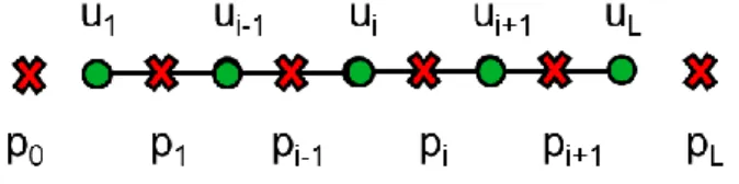
Moreover, a staggered scheme has been chosen for pressure with relation to velocity as illustrated in Fig. 6.

Fig. 6 : Illustration of pressure-velocity discretization scheme.

With this scheme, the pressure derivative at point ui where the velocity is computed, which is

necessary for the momentum conservation equation, gives at the second order:

(18) And at the fourth order:

(19)

This reduces numerical challenges due to solving incompressible flows such as aliasing or other numerical oscillations. The sensibility of the convergence to the discretization scheme is to be studied in further details.

(10)

enthalpy and the void fraction. This means that the equations solved for these unknowns are

hard-coded in the residual vector and Jacobian matrix. The secondary unknowns, such as the mixture density, can be computed as linear combination of the principal unknowns and are therefore solved

explicitly. This allows to improve the solving algorithm's efficiency without compromising the advantages of using an implicit solver. Let us illustrate here a typical member of the Jacobian matrix, which is defined as the derivatives of the equations with respect to the unknowns, here the advection term for the enthalpy equation following the second order discretization scheme:

(20) If we consider the first term only, which is the derivative with respect to the density, we write the derivative of the product as the product of the derivatives:

(21)

(22) As this term is computing the contributions to the Jacobian matrix of this term from the density, we can consider the product uh to be a single unknown. This means that, for each mesh element, three contributions will be added to the Jacobian matrix: , and , and of course even more for the fourth order discretization scheme. One can realise how reducing the number of unknowns and equations to be treated implicitly as well as finding a simpler but mathematically equivalent numerical formulation for these contributions is crucial to the efficiency of the algorithm: as such a 400 elements mesh as used here requires a 1600x1600 Jacobian matrix if we have four unknowns to a 1200x1200 for three implicit unknowns. The added-value of the automatic differentiation as implemented in Diamanlab also becomes clear as it allows the automatic computation of the Jacobian matrix instead of the manual procedure explained above.

3.3. Preliminary Continuation Tests

Some exploratory studies have been led on a homogeneous model, which is a reduced version of the model introduced later in this paper keeping only the three conservation equations written with respect to the mixture parameters, so without drift terms describing the interactions between the phases. The aim was to gain a first insight on the ability of our model to recreate the physics and phenomena involved and on the workings of continuation methods. The parameters, such as phase change enthalpy or density ratio, are arbitrary but chosen so as to be representative of those of a low pressure water flow, itself ressembling those of sodium as far as the liquid/vapour density ratio is seen as a fluid mechanics driving mechanism.

With that in mind, we implemented this simplified model in both ANM and a zero-order continuation method (using the solution at the previous continuation point as the first guess for the current continuation point, without improvement on the prediction) coupled to a Newton-Raphson solving algorithm as the corrector. This latter algorithm will be referred to as zero-order continuation for the rest of this section.

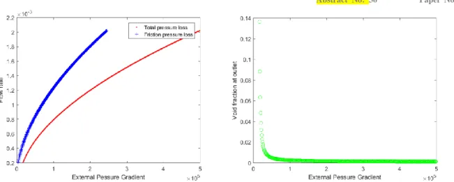
Firstly, we solved our equations written with the mixture velocity as one of the primary unknown with our zero-continuation resolution algorithm. This means we have four unknowns: velocity, pressure, enthalpy and density of the mixture. The continuation parameter was chosen to be the pressure difference between inlet and outlet, as this would be the most realistic for a loss of pump power supply typical of an ULOF transient initiator. This converges for low void fractions only and struggles when we reach a turning point as the branch of solutions is not a bijection at that point anymore: two flow rates coexist as solutions for a single pressure difference and this basic algorithm therefore struggles to converge, as illustrated in Fig. 7. Furthermore, the Jacobian matrix is singular at a turning point, and the zero-order continuation algorithm does not compute the extended system, so it cannot handle that singularity.

(11)

Fig. 7 : Zero-order continuation algorithm, equations written as velocity, pressure difference as continuation parameter.

Secondly, to solve this issue, we rewrote our equations using the mass flux as a primary unknown, instead of velocity and density, hence reducing to 3 the number of primary unknowns. Furthermore, we chose the mass flow rate as the continuation parameter, hence ensuring the unicity of solution for each value of continuation parameter. As a result, the zero-continuation algorithm could draw the whole boiling characteristic curve in one calculation without any convergence problem, as illustrated in Fig. 8.

Fig. 8 : Zero-order continuation algorithm, equations written as mass flux, mass flow as continuation parameter.

Thirdly, we kept the mass flux formulation of the equations as more efficient numerically while equivalent physically. But we changed the continuation parameter back to the pressure difference to be more realistic with an ULOF scenario in mind. This is important because it may have an impact on the nature and weight of the non-linearities and therefore on the final stability. In such configuration, the zero-continuation algorithm was able to draw the boiling characteristic curve in three parts, divided at each of the turning points. It could not indeed find the exact solution at the turning point because the Jacobian matrix is singular there, as illustrated in Fig. 9.

(12)

Fig. 9 : Zero-order continuation algorithm, equations written as mass flux, pressure difference as continuation parameter.

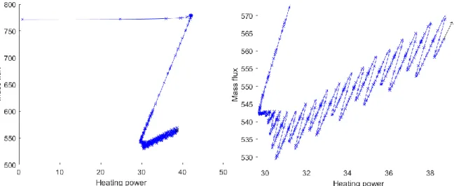
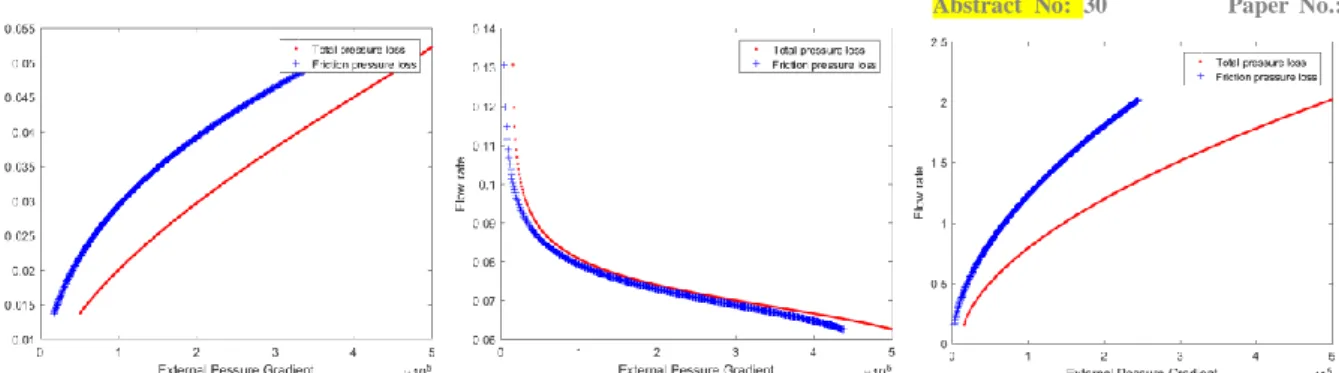
Finally, we implemented the same model in the ANM with the pressure difference as continuation parameter. The ANM draw the whole characteristic curve in one calculation, computing the solution at the turning points as well thanks to its extended system formulation. Moreover, the adaptability to non-linearities allows a substantial reduction of the amount of continuation steps required, from 999 for the zero-continuation algorithm to 38 for the ANM in the same configuration, as illustrated in Fig. 10.

This allows us to illustrate the added-value of the ANM over a classic resolution algorithm, not only ensuring the find all the solutions, even if the branches of solutions are not unique, but also in a more efficient manner.

Fig. 10 : Zero-order continuation (left) vs ANM (right), equations written as mass flux, mass flow as continuation parameter (left), pressure difference as continuation parameter (right).

4. RESULTS

In this section, we apply our approach to the configuration of the experimental campaign led by Saha in the 1970’s in the framework of the R&D for the BWRs [19].

These experiments were designed to study the oscillatory instabilities in a uniformly heated single fluid channel. The fluid used was Freon-113 because of its low critical pressure, hence low boiling point at moderate pressure (typically 149°C at 1.2Mpa) and low latent vaporization heat (14.7*104 J/kg at atmospheric pressure), hence reducing operating costs for a physical behaviour similar to water. The test section is composed of a single vertical cylindrical steal tube of 10mm inner radius heated externally by a DC supply uniformly along its 2.7m height. Valves at the inlet and outlet allow the setting of the throttling in the test section. A large bypass (50mm of diameter) runs paralel to the test section. Instruments were installed to measure flow rate, pressure, temperature and power to the test section.

(13)

versus phase change number introduced by Ishii and Zuber [9], [30]. For each run, hence each stability map, the system pressure, the inlet and outlet valves and the inlet flow rate were kept constant. The large bypass allows the assumption of the total pressure drop remaining constant too. The heating power was increased step by step until sustained oscillations were observed. To obtain several points to plot in one stability map, the inlet subcooling was set thanks to a pre-heater system.

These points were then compared to the equilibrium theory developed by Ishii and Zuber [9], [30] and the non-equilibrium theory of Saha and Zuber [10] as illustrated in Fig. 11.

Fig. 11: Stability map by Saha [19].

To use those experimental results as a comparison basis for our method, we ran simulations in a configuration as close as possible. The physical parameters for Freon-113 in the experimental operating conditions were taken from NIST database1. We fixed the total pressure drop and set the heating power as the continuation parameter. The bifurcation diagram obtained for an Nsub=5 in Fig. 12 does not indicate any specific behaviour.

Fig. 12: Bifurcation diagram in Saha case.

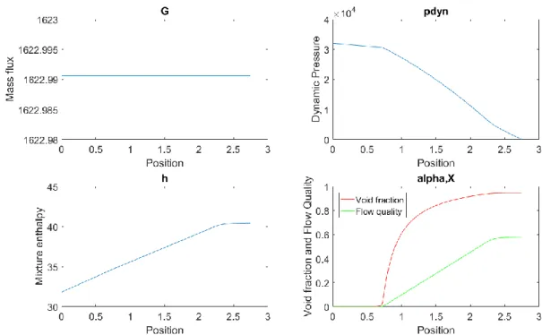
The experiments reported by Saha show the onset of oscillations at Npch=10. The results of our simulation at such operating point are shown in Fig. 13. On the top left the mass flux is plotted versus the axial position. It remains constant indicating the continuity equation is solved correctly. The bottom left shows the enthalpy’s evolution, which is linear along the heated length. It is important to note at this point that we set the heating on only the first four fifths of the length of the channel so as to avoid a strong slope of void fraction close to the outlet, which is likely to destabilize the boundary condition and hence the whole computation. However we do not expect this to have a strong impact on

(14)

the relative weight of non-linearities hence the appearance of oscillations or their stability. The top right figure shows the dynamic pressure. It decreases monotonly along the test section, showing a difference of slope depending on the void fraction as the viscosity evolves, as expected. Finally the bottom right figure illustrates the void fraction and flow quality. The latter fully respects the regularization as a function of enthalpy described earlier while the former shows the impact of the drift velocity. By looking at Eq. (7), which links the void fraction and the flow quality, we see the middle term shows the impact of the drift. This term is proportional to α(1-α), this means that for void fraction lower than 0.5 it has a positive slope, and vice versa for void fractions higher than 0.5. This explains the shape of the void fraction curve.

Fig. 131: Main variables at the point of onset of experimental oscillations.

Saha proposed an analytical model based on these experiments where he uses a constant drift velocity of 0.11ms-1 (corresponding to the application of the correlation from Zuber and Findlay [9] for a bubbly-churn flow) and a constant two-phase wall friction multiplying coefficient of 2. In our model, we set the drift velocity as constant at the same value but we do not use a multiplying coefficient, as explained in the section about the equations. In Fig. 14, we can see the equivalent multiplying coefficient of our model at the point of onset of oscillations according to the experiments. It is clear that our model is not equivalent from this point of view, and it overestimates the wall friction. This is expected to have a stabilizing impact by decreasing the relative weight of the acceleration effects, hence delaying or avoiding the apparition of oscillations.

(15)

Fig. 14: Equivalent two-phase wall friction multiplying coefficient.

Furthermore, our model does not include any pressure drop at inlet or outlet due to the throttling valves of Saha. These differences have an impact on the weight of non-linearities and may explain the lack of oscillations observed in our simulations. Several other sources of non-linearities could also be considered such as the impact of interfacial friction abrupt change connected to flow pattern change (bubbly, slug/churn, annular), a threshold mechanism depending on liquid and vapour volumetric flux.

To illustrate the importance of the relative weight of non-linearities, we have devised an academic study case which differs from the experimental case in the density ratio between the liquid and vapour phase being one order of magnitude higher and both phases viscosities being an order of magnitude higher as well. As a result, we observe in Fig. 15, for similar Nsub and other parameters, oscillations on the bifurcation diagram. This can be related to the Reynolds number. In this scenario, and on the contrary from the Saha paramters, we see a transition from a turbulent to a laminar regime by crossing the value Re=2300, which is the limit in the Churchill law we use. This means a non-linearity due to the flow regime transition appears and may trigger these oscillations that can be seen as the onset mechanism of density waves oscillations in an incompressible flow solved without the time-related terms of the equations.

Fig. 152: Bifurcation diagram of Academic case with apparition of oscillations.

As explained when describing the equations of our model, their pure advective nature means temporal oscillations such as density waves are transposed into spatial oscillations like those observed in Fig. 15. Nevertheless, a proper stability analysis based on the eigenvalues of our set of equations is required to

(16)

and its stability, as was already explored in [18]. Using the mathematical definitions introduced in the section about the Theory of Dynamical Systems, we know such an analysis requires the writing and solving of a monodromy matrix in addition to the Jacobian matrix. This requires some additional work. A sensibility study of the stability analysis to the impact of such monodromy matrix compared to the use of the Jacobian matrix on its own is considered so as to quantify the necessity of this monodromy matrix. On a simplified case of our model, we have shown our ability to detect the change from non-imaginary eigenvalues to conjugated non-imaginary eigenvalues, which is typical of a Hopf bifurcation.

5. CONCLUSIONS

This paper presented the work achieved during the first half of a PhD work at the CEA and Aix-Marseille University on the stability and bifurcation analysis of sodium boiling. In regard to the highly dynamical and non-linear phenomenology observed in previous studies at the CEA, a semi-analytical method based on the ANM is developped to get an efficient and rigorous solution of the governing non-linear equations. It enables to find all steady-state solutions and among them those of particular interest (bifurcation points) where a stability analysis has to be performed. The relevant mathematical highlights from the Theory of Dynamical Systems have been reported to support the inner workings of the approach which have been detailed. The added-value and feasibility are illustrated. A model based on the classical drift model from the literature is used to describe the physics involved, but some modifications have been introduced to fit the demands requirements of our semi-analytical approach. The resulting numerical model has been run in different continuation configurations, such as mass flow rate or pressure drop imposed at the boundaries, which are indeed representative of experiments from the literature and reactors’ ones along a loss of flow transient. Interestingly, the method has proven capable of handling such a variety of situations. A validation case on experiments led by Saha in the 1970’s has been investigated so as to balance the predictive ability of the model regarding two phase flow stability boundary. The simulations using the experimental parameters have shown no sign of oscillations on the bifurcation diagram. However, an academic scenario with a different ratio between the non-linearities has been used to trigger oscillations – which are seen as prototypic of a density wave mechanism onset – on the bifurcation diagram. The validity of these indicators is to be verified by a linear stability, which is actually the only appropriate methodology to identify them. Moreover, in the Saha experimental case, the closure laws and effects of the singularities have to be studied to evaluate their possible role regarding the onset of density wave mechanism that was observed.

Investigating the ability of the present model to reproduce a stability boundary comparable to the one reported by Saha with his drift model, while using the same set of parameters and closure laws is indeed a key step to the understanding of the phenomenology observed in the experiments.

For the second half of this PhD work, several directions will be investigated. Firstly, sensibility studies to the closure will be led, as there are many formulations proposed in the literature and it would be enlighting to gain a better understanding of their validity range on our specific study case. Secondly, sensibility studies focusing on the characteristics of a typical CFV reactor case are considered. This includes a rapid change of hydraulic diameter or a coupling between power and void fraction. Finally, the stability study method needs further development with the inclusion of a monodromy matrix and a sensibility study to the different approaches of linear stability study.

NOMENCLATURE a. Roman Letters

Letter Definition Units

D Diameter m

f Generic function /

(17)

g Gravity acceleration m.s-2

h Enthalpy J.kg-1

I Identity matrix /

i Index of current discretization point /

J Jacobian matrix / P Pressure Pa q Heating flux W.m-2 u Velocity m.s-1 w Perturbation amplitude / X Vapour quality / y Generic solution /

ys Generic stationary solution /

z Position m

b. Greek Letters

Letter Definition Units

α Void fraction /

Δ Differential of the unknown /

ε Approximation error /

λ Eigenvalue or continuation parameter / or /

μ Viscosity or perturbation frequency Pa.s or /

ρ Density Kg.m-3 c. Indices Index Definition H Hydraulic l Liquid phase m Mixture v Vapour phase w Wall

ACKNOWLEDGMENTS

We would like to make a special mention to managers of CNRS and CEA making this PhD

work possible in the frame of CEA-AMU agreement, CEA project for SFRs for the PhD

financement, and the laboratory head for his commitment in the release process of this paper.

REFERENCES

[1] M. Chenaud et al., ‘Status of the ASTRID core at the end of the pre-conceptual design phase 1’,

Nuclear Engineering and Technology, vol. 45, no. 6, pp. 721–730, Nov. 2013.

[2] J. M. Seiler, ‘Studies on sodium-boiling phenomena in out-of-pile rod bundles for various accidental situations in LMFBR: Experiments and interpretations’, Nuclear Engineering and

Design, vol. 82, no. 2/3, pp. 227–239, 1984.

[3] H. M. Kottowski and C. Savatteri, ‘Fundamentals of liquid metal boiling thermohydraulics’,

ResearchGate, vol. 82, no. 2, pp. 281–304, Oct. 1984.

(18)

two-Abstract No: 30 Paper No.:

fluid model computer code SABENA’, Nuclear Engineering and Design, no. 97, pp. 233–246, 1986.

[5] J. M. Seiler, D. Juhel, and P. Dufour, ‘Sodium boiling stabilisation in a fast breeder subassembly during an unprotected loss of flow accident’, Nuclear Engineering and Design, vol. 240, no. 10, pp. 3329–3335, Oct. 2010.

[6] J. Perez, N. Alpy, D. Juhel, and D. Bestion, ‘CATHARE 2 simulations of steady state air/water tests performed in a 1:1 scale SFR sub-assembly mock-up’, Annals of Nuclear Energy, vol. 83, pp. 283–297, Sep. 2015.

[7] N. Alpy et al., ‘Phenomenological investigation of sodium boiling in a SFR core during a postulated ULOF transient with CATHARE 2 system code: a stabilized boiling case’, Journal of

Nuclear Science and Technology, vol. 53, no. 5, pp. 692–697, May 2016.

[8] R. W. Lockhart and R. C. Martinelli, ‘Proposed Correlation of Data for Isothermal Two-Phase, Two-Component Flow in Pipes’, Chemical Engineering Progress, vol. 45, no. 1, pp. 39–48, Jan. 1949.

[9] N. Zuber and J. A. Findlay, ‘Average Volumetric Concentration in Two-Phase Flow System’,

Journal of Heat Transfer, pp. 453–468, Nov. 1965.

[10] P. Saha and N. Zuber, ‘An analytical study of the thermally induced two-phase flow instabilities including the effect of thermal non-equilibrium’, International Journal of Heat and Mass Transfer, vol. 21, no. 4, pp. 415–426, Apr. 1978.

[11] M. Ishii, ‘One-dimensional Drift-flux Model and Constitutive Equations for Relative Motion between Phases in Various Two-phase Flow Regimes’, Argonne National Laboratory, vol. 77, no. 47, Oct. 1977.

[12] T. Hibiki and M. Ishii, ‘One-dimensional drift-flux model and constitutive equations for relative motion between phases in various two-phase flow regimes’, International Journal of Heat and

Mass Transfer, vol. 46, no. 25, pp. 4935–4948, Dec. 2003.

[13] T. Hibiki and M. Ishii, ‘Erratum to: “One-dimensional drift-flux model and constitutive equations for relative motion between phases in various two-phase flow regimes” [International Journal of Heat and Mass Transfer 46 (2003) 4935–4948]’, ResearchGate, vol. 48, no. 6, pp. 1222–1223, Mar. 2005.

[14] Rizwan-uddin and J. J. Doming, ‘A Chaotic Attractor in a Periodically Forced Two-Phase Flow System’, NSE, vol. 100, no. 4, pp. 393–404, Dec. 1988.

[15] J. A. Boure, A. E. Bergles, and L. S. Tong, ‘Review of Two-Phase Flow Instability’, Nuclear

Engineering and Design, vol. 25, pp. 165–192, 1973.

[16] S. Kakac and B. Bon, ‘A Review of two-phase flow dynamic instabilities in tube boiling systems’,

International Journal of Heat and Mass Transfer, vol. 51, no. 3–4, pp. 399–433, Feb. 2008.

[17] C. Lange, D. Hennig, and A. Hurtado, ‘An advanced reduced order model for BWR stability analysis’, Progress in Nuclear Energy, vol. 53, no. 1, pp. 139–160, Jan. 2011.

[18] E. Bissen, N. Alpy, and M. Medale, ‘Stability and Bifurcation Analysis of Sodium Boiling in a GEN IV SFR Reactor Core’, presented at the FR17 Conference on Fast Reactors and Related Fuel Cycles, Iekaterinburg, Russia, 2017.

[19] P. Saha, M. Ishii, and N. Zuber, ‘An Experimental Investigation of the Thermally Induced Flow Oscillations in Two-Phase Systems’, J. Heat Transfer, vol. 98, no. 4, pp. 616–622, Nov. 1976. [20] R. Seydel, ‘Nonlinear Computation’, Int. J. Bifurcation Chaos, vol. 07, no. 09, pp. 2105–2126,

Sep. 1997.

[21] E. Doedel, ‘Nonlinear Numerics’, Int. J. Bifurcation Chaos, vol. 07, no. 09, pp. 2127–2143, Sep. 1997.

[22] R. Seydel, Practical Bifurcation and Stability Analysis, Springer. 1994.

[23]H. B. Keller, ‘Nonlinear bifurcation’, Journal of Differential Equations, vol. 7, no. 3, pp. 417–434, May 1970.

[24] B. Cochelin, N. Damil, and M. Potier-Ferry, Méthode asymptotique numérique, Lavoisier. 2007. [25] E. Hopf, ‘Abzweigung einer periodischen Losung von einer stationaren Losung eines

Differentialsystems’, Berichten der Mathematisch-Physischen Klasse der Sachsischen Akademie

der Wissenschaften zu Leipzig, vol. XCIV, pp. 1–22, 1942.

[26] I. Charpentier, B. Cochelin, and K. Lampoh, ‘Diamanlab - An interactive Taylor-based continuation tool in MATLAB’, 2013.

(19)

[27] G. Yadigaroglu, ‘Instabilities in two-phase flow’. ETH Zurich, Short Course on Modelling and Computation of Mulitphase Flows, Feb-2012.

[28] J.-M. Delhaye, Thermohydraulique des réacteurs, EDP Sciences. 2008.

[29] S. W. Churchill, ‘Friction Factor Equations Spans All Fluid-Flow Regimes’, Chemical

Engineering Journal, vol. 84, no. 24, pp. 91–92, 1977.

[30]M. Ishii, ‘Thermally induced flow instabilities in two-phase mixtures in thermal equilibrium’, Aug. 1971.